Transport on coupled spatial networks

Abstract

Transport processes on spatial networks are representative of a broad class of real world systems which, rather than being independent, are typically interdependent. We propose a measure of utility to capture key features that arise when such systems are coupled together. The coupling is defined in a way that is not solely topological, relying on both the distribution of sources and sinks, and the method of route assignment. Using a toy model, we explore relevant cases by simulation. For certain parameter values, a picture emerges of two regimes. The first occurs when the flows go from many sources to a small number of sinks. In this case, network utility is largest when the coupling is at its maximum and the average shortest path is minimized. The second regime arises when many sources correspond to many sinks. Here, the optimal coupling no longer corresponds to the minimum average shortest path, as the congestion of traffic must also be taken into account. More generally, results indicate that coupled spatial systems can give rise to behavior that relies subtly on the interplay between the coupling and randomness in the source-sink distribution.

Systems that can be represented as a group of interacting networks are found everywhere in modern life MH01 ; SMR+04 ; VRLI+08 . From so-called smart power grids—which couple electrical distribution networks with ICT control networks VV+10 —to interactions between other types of critical infrastructure networks, such as food and water supply, transport, fuel, and financial transactions. Recent theoretical studies on the subject have generated a great deal of interest by demonstrating that coupling two or more networks together can lead to system-wide behaviour which differs fundamentally from the behaviour of each individual network RP+10Jul ; SVB+10Apr ; XHJG+11 ; CG+11Aug ; JGSB+11 ; CDB+12Feb ; CDB+12Apr ; Boguna:2012 ; resp1 ; resp2 . These studies describe essentially cascade-like processes where typically either inverse-percolation SVB+10Apr ; JGSB+11 ; CDB+12Apr or sandpile methods CDB+12Feb are used (or variants thereof). In the former case, the robustness of the system is characterized by size of the remaining giant connected component, whilst for the latter, it is the size of the largest sand-cascade. In both cases, the quantity of interest is directly related to the topology of the network and does not permit any consideration of dynamical processes which may take place on the network. Furthermore, robustness against cascade failures is not the only consideration for those affected by such real world systems.

One broad class of processes that occur on a network are general transport processes, or flows SC+08Oct . Whether flows of people, fluids, or electrical currents, these systems can be characterized by specifying the topology of the underlying network, a source-sink distribution, and a dynamic (Fig. 1). Where, to avoid confusion, we only imagine dynamical processes that converge to a steady state—resulting in a stationary distribution of flows over the network. Unfortunately, the methods of analysis mentioned above do not capture many of the typical features one might expect here. For example, it is easy to imagine a simple source-sink distribution that allows the network to be split into two distinct components such that the flows are unaffected. In this case, the size of the giant component may decrease but the network is still operating well. With this example in mind, one question that arises is: how should an interacting, or coupled, set of flow networks be characterized, and what are the interesting features of such systems? Whilst any system-wide behaviour is intimately linked with the particular dynamics, some understanding can be gained by investigating the properties of simple examples that are chosen well enough to represent some sub-class of these systems. In this study, we report the results of investigating such a toy model, and highlight the interesting features which we believe might be typical of many problems in this class.

Figure 1: (Color online) A system made of two coupled networks where the nodes of network 2 form a subset of the nodes of network 1. Edges of network 1 are shown in black, edges of network 2 are shown in red (gray offline), and nodes in common to both networks are considered to be coupled (shown by dashed lines). Highlighted in green (gray offline), we represent a path between two nodes, the “source” $i$ and the “sink” $j$.

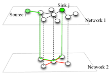
Most existing studies of coupled networks focus on variants of the random graph SVB+10Apr ; CDB+12Feb ; CDB+12Apr , primarily due to the simplicity with which properties can be calculated. However, many physical networks (i.e., electrical, transportation, ICT etc.) are spatial networks and are often planar MB11 . For this reason, this letter focusses on coupled planar networks. Although, for completeness, the example of spatially embedded Erdős-Rényi random networks is discussed later alongside the results for the planar case. In addition to this, coupled networks are usually found to be linked by a set of nodes common to both networks (note that this is however not a necessary limitation of the model, but simply a more realistic assumption for spatial networks). For example, this is the case for a road network coupled to a rail or subway network. Here, all the nodes of the road network are not nodes of the rail network, but conversely, all stations are located at points which can be considered as nodes in the road network. Motivated by this simple example, we construct a first planar network as a triangulation of points in the plane. Triangulations are often used as a convenient way to generate planar networks from a given distribution of nodes. We choose the usual Delaunay triangulation LGJS85 , which typically avoids slim triangles—not seen very often in real networks due to their inefficiency—and which is effectively unique for a given set of points. We then construct a second network based on a random subset of the points used to construct the first network. Our model thus comprises individual networks that are each planar Delaunay triangulations, forming a combined network that is not necessarily planar (see Fig. 2) and where the nodes of the different networks with the same spatial location are linked together.

Figure 2: (Color online) Each instance of the system is generated according to the following process: 2 First, $N_{1}$ nodes (here $N_{1}=30$) are positioned at random within the unit circle and the Delaunay triangulation is produced; 2 the second network is then generated by drawing $N_{2}$ (here $N_{2}=10$) nodes uniformly from the existing ones ($N_{2}\leq N_{1}$) and, once again, computing the Delaunay triangulation; 2 the combined system is no longer planar and can be represented as a top-down view of Fig. 1 (where zero weights assigned to the dotted interconnecting lines).

Rather than considering a dynamical system which acts to minimize a global quantity—such as electrical networks, where the dissipated power is minimized—we allocate flows on the network following a basic transportation analogy. Here, the source-sink distribution is replaced by an origin-destination (OD) matrix $T_{ij}$. This has the benefit that it explicitly specifies the flow between node $i$ and node $j$. Therefore all that remains is to decide a method of route assignment. The obvious choice is to use the weighted shortest path, where the number of such paths between nodes $i$ and $j$ is denoted by $\sigma_{ij}$. In our model, the weight associated with each edge is the length of that edge multiplied by a factor $0\leq\alpha_{n}\leq 1$, which is common to all edges belonging to the same network. The subscript $n$ is used to label the network: $n=1$ corresponds to the larger network and $n=2$ the smaller. The idea is that $\alpha=\alpha_{2}/\alpha_{1}$ is a single parameter that controls the relative weight per unit distance between the two networks. Indeed, in order to simplify further, we impose the artificial constraint that $\alpha\leq 1$. This has the effect that a journey on the smaller network ($n=2$) is favored over a journey of equivalent distance for the larger network ($n=1$). We also note that since the edge weights are proportional to edge length and nodes are positioned at random, it is very unlikely that $\sigma_{ij}>1$.

Previous studies of interacting networks use the term coupling to describe how well two networks are linked. Typically, this is a purely topological definition i.e., the fraction of nodes from one network which link to another RP+10Jul , or the probability that a particular node has an edge which connects both networks CDB+12Feb . For transport processes, a better measure of interaction must include details of how the flows are distributed. For the system outlined above we define the coupling as

$$\lambda\equiv\sum_{i\neq j}T_{ij}\frac{\sigma_{ij}^{\mathrm{coupled}}}{\sigma_{ij}},$$ (1)

where $\sigma_{ij}^{\mathrm{coupled}}$ is the number of shortest paths between nodes $i$ and $j$, which include edges from both networks, and where the entries of the origin-destination matrix $T_{ij}$ are normalized i.e., $\sum_{ij}T_{ij}=1$. It is clear from Eq. (1) that $\lambda\in[0,1]$ is just the fraction of travellers that use both networks. Such a definition is dependent on the method by which the flows are allocated and not just on the system topology. Indeed, for a given allocation method and network topology, there is usually a maximum value of $\lambda$ strictly less than one. In our model, the coupling is controlled by choosing $\alpha$. By virtue of changing the weights associated with each network, $\alpha$ changes the (weighted) shortest path between any two nodes. For example, a value of $\alpha$ close to one indicates little difference between the two networks and hence, on average, shortest paths do not utilize both networks. By contrast, a low value of $\alpha$ (close to zero) gives rise to significantly lower weights on the second network and therefore shortest paths typically use both networks.

With Eq. (1) in mind, instead of investigating the likelihood of catastrophic cascade failures, we consider more general measures of how well the system is operating. For example, one such measure is the average distance travelled

$$\bar{d}=\sum_{i\neq j}T_{ij}d_{ij},$$ (2)

where $d_{ij}$ is the distance travelled between nodes $i$ and $j$. For most practical transport processes, a well designed system reduces the average distance travelled (i.e., water/food supply, the Internet, transportation, etc.). Another important quantity, which is a simple proxy for traffic, is the edge betweenness centrality, defined as $x_{e}=\sum_{i\neq j}T_{ij}\left(\sigma_{ij}\left(e\right)/\sigma_{ij}\right)$, where subscript $e$ is used to label edges, and $\sigma_{ij}\left(e\right)$ is the number of shortest paths between nodes $i$ and $j$, which use edge $e$. The betweenness centrality allows us to introduce a second measure we are concerned with, the Gini coefficient $G$. A number between zero and one, $G$ is typically used in economics for the purpose of describing the distribution of wealth within a nation. Here it is used to characterize the disparity in the assignment of flows to the edges of a network, something that has been done before for transportation systems such as the air traffic network AR-F01 . For example, if all flows were concentrated onto one edge, $G$ would be one, whilst if the flows were spread evenly across all edges, $G$ would be zero. We use the definition according to Ref. gini

$$G\equiv\frac{1}{2E^{2}\bar{x}}\sum_{p}\sum_{q}|x_{p}-x_{q}|,$$ (3)

where subscripts $p$ and $q$ label edges, $E$ is the total number of edges, $x_{p}$ is the flow assigned to edge $p$ as defined earlier, and $\bar{x}=\sum_{p}x_{p}/E$ is the average flow on an edge.

Unfortunately, it is impractical to consider the interplay between $\lambda$, $\bar{d}$, and $G$, for all possible OD matrices. Therefore it helps to choose a specific example. We start with a monocentric OD matrix—i.e., all nodes travel to the origin—and then add noise by rewiring in the following way. For each node, with probability $p$, choose a random destination, and with probability $1-p$, choose the origin (see Fig. 3).

Figure 3: (Color online) Representations of OD matrices where each arrow corresponds to an entry in $T_{ij}$ and which relates to the set of points in Fig. 2. 3 A monocentric OD matrix. 3 A monocentric OD matrix randomly rewired with probability $p=0.5$.

The set of numbers $N_{1}$, $N_{2}$, $p$, and $\alpha$, now define an ensemble of systems that are statistically equivalent (with respect to $\lambda$, $\bar{d}$, and $G$). We proceed by calculating the quantities $\langle\lambda\rangle$, $\langle\bar{d}\rangle$, and $\langle G\rangle$ for different values of $p$ and $\alpha$, where angle brackets $\langle\dots\rangle$ represent an ensemble average. The results are shown in Fig. 4, where each data point corresponds to an average over fifty instances of the OD matrix for each of fifty instances of the coupled network geometry.

Figure 4: (Color online) Simulation results for the average shortest path and the Gini coefficient ($N_{1}=100$, $N_{2}=20$, and $p$ values: $0$ (purple dots), $0.2$ (blue squares), $0.4$ (green diamonds), $0.6$ (orange triangles), and $0.8$ (red inverted triangles)). When the coupling increases, the average shortest path decreases and the Gini coefficient can increase for large enough disorder.

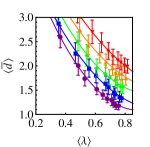
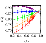
We find that, as the coupling increases, the length of the average shortest path decreases (Fig. 4). This is straightforward to understand since the increased coupling is simply a result of reducing $\alpha$. Furthermore it is clear that increasing randomness in the origin destination matrix increases the length of the average shortest path by an almost constant value, irrespective of the coupling. By contrast, the behaviour of the Gini coefficient at different couplings (Fig. 4) is less easily explained. Consider instead Fig. 5. Here, each colormap shows the distribution of flows resulting from many instances of the system.

Figure 5: (Color online) Colormaps showing normalized edge flows—plotted at the midpoint of each edge—over many instances of the system. Colors are assigned from lightest to darkest, starting with white (for zero flow) and moving through yellow, orange and red for higher values of flow, until reaching black (maximum flow). Each Subfigure corresponds to the following parameter values: 5 $p=0.2$, $\alpha=0.9$; 5 $p=0.2$, $\alpha=0.1$; 5 $p=0.8$, $\alpha=0.9$; 5 $p=0.8$, $\alpha=0.1$.

The first two plots, Figs. 5 and 5, were generated from OD matrices rewired with low probability ($p=0.2$) i.e., almost monocentric. The ratios of edge weights per unit distance between the two networks are $\alpha=0.9$ and $\alpha=0.1$ respectively. Therefore each diagram corresponds to a point on the blue line in Fig. 4. For $\alpha=0.9$, there is minimal coupling between the networks and a high concentration of flows are seen around the origin. Since the flows are disproportionately clustered, this configuration is described by a high Gini coefficient. By contrast, for $\alpha=0.1$, the difference in the edge weights means that it can be beneficial to first move away from the origin in order to switch to the ‘fast’ (low $\alpha$) network. We therefore see a broader distribution of flows with small areas of high concentration around coupled nodes. The emergence of these hotspots away from the center also corresponds to a high Gini coefficient—and therefore the blue line in Fig. 4 is relatively flat. Figs. 5 and 5 correspond to the red line of Fig. 4: generated from OD matrices rewired with high probability ($p=0.8$). We observe that even for $\alpha$ close to one, the localization of flows is less than for $p=0.2$—resulting in a lower Gini coefficient. As $\alpha$ is decreased, the second network becomes more favourable and coupling hotspots can be seen once again—resulting in a high Gini coefficient and a positive gradient for the red line of Fig. 4. This result points to the general idea that randomness in the source-sink distribution leads to local congestion and more generally to a higher sensitivity to coupling.

Heuristically, one might consider this a simple model of a two mode transportation system in the low density regime—i.e., where the effects of congestion do not affect route choice. We imagine a road network coupled to a rail network where users select the quickest route to their destination. That is, the shortest path actually represents the quickest path. This implies that the scale factors $\alpha_{\mathrm{road}}$ and $\alpha_{\mathrm{rail}}$ must have units of time divided by distance, so we assume that they represent the inverse of the average speed associated with each mode. The result is that decreasing (increasing) the ratio of these factors, $\alpha$, has the effect of increasing (decreasing) the relative speed of rail above road—and hence the coupling. In this picture, the Gini coefficient can now be thought of as a measure of road use. A low value indicates that the system uses all roads to a similar extent, whilst a high value indicates that only a handful of roads carry all the traffic. With this analogy in mind, it is natural to combine the effects observed above into a single measure. We assert that it is likely that a designer or administrator of a real system would wish to simultaneously reduce the average travel time and minimize the disparity in road utilization. To serve this purpose, we define a ‘utility’ function $F=\langle\bar{d}\rangle+\mu\langle G\rangle$, where it is immediately apparent from Fig. 4 that, for certain values of $\mu$, the function $F$ will have a minimum. That is, a non-trivial (i.e., non-maximal) optimum $\lambda$ will emerge. Figure 6 shows that, whether a non-trivial optimum coupling exists depends on the origin-destination matrix. For OD matrices rewired with a high probability, increasing the speed of the rail network reduces the road utilization as flows become concentrated around nodes where it is possible to change modes. Dependent on the value of $\mu$, the effect of reduced utilization can outweigh the increased journey time, leading to a minimum in $F$. Monocentric OD matrices, by contrast, have inherently inefficient road utilization when applied to planar triangulations, regardless of the speed of the rail network. Therefore no minimum is observed, and hence no (non-trivial) optimum $\lambda$.

Figure 6: Existence of an optimal coupling: 6 Simulation results for $\mu=10$, $N_{1}=100$, $N_{2}=20$, and $p$ values: $0$ (purple dots), and $0.8$ (red inverted triangles) (only two values of $p$ are shown to ensure the lines of best-fit can be seen clearly). 6 Minima of quadratic best-fit curves for different values of $p$. We obtain $p^{*}\simeq 0.32$ using a straight-line approximation between the two closest points, above and below, $\lambda^{*}=1$. (The error bars shown are those of the closest data point to the minimum of the best-fit curve).

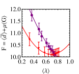
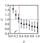
More systematically, we plot in Fig. 6 the minima $\lambda^{*}(p)$ of quadratic best-fit curves obtained from Fig. 6, each corresponding to a different value of $p$. Defining $p^{*}$, the value of $p$ for which $\lambda^{*}(p^{*})=1$, it is possible to categorize the system into one of two regimes. We observe that: if $p<p^{*}$, then the optimal coupling is trivially the maximum; otherwise if $p\geq p^{*}$, a non-trivial optimal coupling exists.

Finally, we note that similar effects can be observed on other non-planar networks. As mentioned earlier, one example is Erdős-Rényi random networks generated for a set of nodes with random locations. Whilst the observed behaviour is qualitatively the same, the results are much less pronounced due to the absence of spatial structure and the spatial localization of centrality.

In conclusion, the model is characterised by two competing forces—the desire to move all flows onto the most efficient network, whilst also ensuring that congestion does not arise around the nodes which connect both networks. We observe that the optimisation of such a system can be sensitive to randomness introduced in the origin-destination matrix. The broader interpretation of our work is that, spatial, space-filling, networks such as transportation networks or the electricity grid, may be inherently fragile to certain changes in supply and demand, such as the transition from centralized power generation to decentralized prosumers IL+10 . This behaviour is not captured by the existing literature, and demonstrates an alternative view of transport processes on interacting networks. Indeed, whilst the assumptions made have a convenient interpretation in terms of bimodal transportation systems, we expect that the results hold for a broader class of systems and welcome work in this area.

Acknowledgements. RGM thanks the grant CEA$/$DSM-Energie for financial support.

References

- (1) M. Heller, The Bridge (Natl. Acad. Eng.) 31, 9 (2001).
- (2) S. Rinaldi, J. Peerenboom, and T. Kelly, IEEE Control. Syst. Magn. 21, 11 (2001).
- (3) V. Rosato, L. Issacaroff, F. Tiriticco, S. Meloni, S. Porcellinis, and R. Setola, Int. J. Crit. Infrastruct. 4, 63 (2008).
- (4) V. Vyatkin, G. Zhabelova, N. Higgins, M. Ulieru, K. Schwarz, and N.-K. C. Nair, 2010 Innovative Smart Grid Technologies (ISGT) (IEEE, New York, 2010), pp. 1–9.
- (5) R. Parshani, S. Buldyrev, and S. Havlin, Phys. Rev. Lett. 105, (2010).
- (6) S. V. Buldyrev, R. Parshani, G. Paul, H. E. Stanley, and S. Havlin, Nature (London) 464, 1025 (2010).
- (7) X. Huang, J. Gao, S. V. Buldyrev, S. Havlin, and H. E. Stanley, Phys. Rev. E 83, 065101(R) (2011).
- (8) C.-G. Gu, S.-R. Zou, X.-L. Xu, Y.-Q. Qu, Y.-M. Jiang, D. R. He, H.-K. Liu, and T. Zhou, Phys. Rev. E 84, 026101 (2011).
- (9) J. Gao, S. V. Buldyrev, H. E. Stanley, and S. Havlin, Nature Phys. 8, 40 (2011).
- (10) C. D. Brummitt, R. M. D’Souza, and E. A. Leicht, Proc. Natl. Acad. Sci. USA 109(12) (2012).
- (11) C. Brummitt, K.-M. Lee, and K.-I. Goh, Phys. Rev. E 85, 045102(R) (2012).
- (12) A. Saumell-Mendiola, M. A. Serrano, M. Boguna, arXiv:1202.4087, (2012).
- (13) W. Li, A. Bashan, S. V. Buldyrev, H. E. Stanley, and S. Havlin, Phys. Rev. Lett. 108, 228702 (2012).
- (14) A. Bashan, Y. Berezin, S. V. Buldyrev, and S. Havlin, arXiv:1206.2062, (2012).
- (15) S. Carmi, Z. Wu, S. Havlin, and H. E. Stanley, Europhys. Lett. 84, 28005 (2008).
- (16) M. Barthelemy, Phys. Rep. 499, 1 (2011).
- (17) L. Guibas and J. Stolfi, ACM T. Graphic. 4, 74 (1985).
- (18) A. Reynolds-Feighan, J. Air Transp. Manag. 7, 265 (2001).
- (19) P. M. Dixon, J. Weiner, T. Mitchell-Olds, and R. Woodley, Ecology 68, 1548 (1987).
- (20) I. Lampropoulos, G. M. A Vanalme, W. L Kling, ISGT Europe 2010 IEEE PES (IEEE, New York, 2010).