Correlated domains in spin glasses

Abstract

We study the $3D$ Edwards-Anderson spin glasses, by analyzing spin-spin correlation functions in thermalized spin configurations at low $T$ on lattices of sizes up to $32^{3}$. We consider individual disorder samples and analyze connected clusters of very correlated sites: we analyze how the volume and the surface of these clusters increases with the lattice size. We qualify the important excitations of the system by checking how large they are, and we define a correlation length by measuring their gyration radius. We find that the clusters have a very dense interface, compatible with being space filling.

1 Introduction

The understanding of the low temperature behavior of spin glass systems [1] is both a very interesting and challenging problem and one of the most relevant open questions in classical statistical mechanics. The mean field theory of the model has been solved [2], and the rigorous mathematical proof that this solution is correct [3] made the situation very clear. In finite dimensional spin glass however, the situation is completely open, and there is no general agreement on what happens in the infinite volume limit ($V\to\infty$). The two main possibilities are on one side that in a finite dimension the model behaves as in mean field [2] (this is the replica symmetry breaking, RSB, picture), by preserving all or most of the very peculiar features of the mean field theory, and on the other side that the so called droplet picture [4] (where only two stable states are relevant for the critical behavior of the system) is realized. For some detailed analysis of the two points of view see for example [5, 6]. The TNT scenario [6] suggests an intermediate situation (the trivial-non-trivial picture) where the link overlap does not have a complex behavior; here we only estimate the usual overlap. Even if it is very plausible that the final answer to this crucial question will not come from numerical experiments, it is clear that today large scale, large volume, very accurate numerical simulations can allow to at least approach the relevant low $T$, large $V$, regime, and give very relevant hints about the physical behavior of such systems in the thermodynamic limit. The numerical simulations of the Janus supercomputer [8, 9, 10, 11] (a special purpose computer [12] specially built to simulate very effectively spin systems with discrete variables and couplings) have produced a large set of well thermalized spin glass configurations on large (since we are considering spin glasses: the same lattice sizes would not be so large for, say, an Ising model with random field) systems at low $T$: our analysis will be based on these spin configurations.

We take the approach, that has been discussed in [13], of considering local magnetizations and correlation functions for a given disorder sample (without averaging over the disorder). This approach can give a very complete picture, and allow detecting important features of the system. We will mainly use spin-spin correlation functions, $k_{i,j}^{(J)}\equiv\langle\sigma_{i}\sigma_{j}\rangle$ (where the brackets indicate the thermal average, $i$ and $j$ are two lattice sites, and $(J)$ denotes a given realization of the couplings) and build upon how much two sites are correlated in a given sample.

Using the values of the $k_{i,j}$ we will build connected clusters of correlated spins. These clusters are related to excitations that during the dynamics tend to move in a coherent way: their spins are very correlated. In this sense these connected  clusters are good proxies of droplets and studying their properties allows us to get information about the droplets. In ref. [14] a similar approach was taken to study excitations at $T=0$. It is thanks to the availability of well-thermalized configurations from Janus for many disorder realizations that we are able to analyze the finite small $T$ region.

2 Model and data analysis

We study here the $3D$ Edwards Anderson spin glass with binary couplings. We analyze well thermalized, equilibrium spin configurations obtained with large scale numerical simulations by the Janus collaboration [8, 9] based on parallel tempering [15] (see ref. [8, 9] for all the parameters of the numerical simulation). We deal with $O(1000)$ samples of quenched disorder and many independent spin configurations per disorder sample (for each lattice size), on simple cubic lattices of sizes going up to $V=L^{3}=32^{3}$, for temperatures down to $0.64\;T_{c}$, with periodic boundary conditions.

For a given disorder sample and lattice site $i$, we form the (connected) cluster ${\cal C}_{i}$ by adding recursively to ${\cal C}_{i}$ all sites $j$ whose correlation function $\langle\sigma_{j}\sigma_{i}\rangle$ is larger in absolute value than a given threshold ${\cal T}_{{min}}$. When this is done, we only keep the connected component containing the site $i$. The value of the threshold ${\cal T}_{{min}}$ is an important parameter of our construction: if it is very small the cluster will fill all the available space, and it will have no boundary, while if it is very large ${\cal C}_{i}$ will be small (but its complement, formed from all lattice sites that do not belong to ${\cal C}_{i}$, will be large). We would expect that in the physically relevant range of values of ${\cal T}_{{min}}$ the universal results of our computation (like, for example, the critical exponents) should not depend on ${\cal T}_{{min}}$, and we will verify that this is indeed the case.

For a given sample we will consider both the set of the $V$ (connected) clusters ${\cal C}_{i}$, analyzing their volume $N_{i}$ and their surface $S_{i}$ (defined as the size of the set of sites which belong to the cluster and have at least one first neighboring site that does not belong to it), and properties obtained by averaging over the different clusters ${\cal C}_{i}$ (e.g. the cluster average volume $N$ and average surface $S$). All these quantities should be labeled also with an index $(J)$, denoting the disorder sample we are considering, but we will omit this label for the sake of a clearer notation. We will try to determine how quantities like $N$ and $S$ scale with the lattice size.

3 Size and surface of connected clusters

Figure 1: In figures 1.(a) and 1.(b) we plot the quantities $S_{i}/V$ versus $N_{i}/V$ for all clusters ${\cal C}_{i}$ ($i=1,\;...,\;V$) for two representative disorder samples. Symbols of different colors and shapes are used (like in figures 1.(c) and 1.(d)), for different values of the threshold ${\cal T}_{{min}}$: black squares are for a threshold of $0.5$, cyan triangles pointing down $0.6$, blue triangles pointing up $0.7$, green circles $0.8$ and red squares $0.9$. In figure 1.(c) we show averages over all clusters ${\cal C}_{i}$ for a given sample (each point is for a given disorder realization, all disorder realizations are plotted), under the constraint $\lambda=0.5$ (see text): in figure 1.(d) we restrict the average to percolating clusters ($\lambda=0.5$).

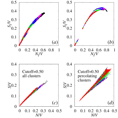
We start by showing what happens in two representative disorder samples in figure 1.a and 1.b. Both figures are scatter plot that shows the cluster surface density $s_{i}\equiv S_{i}/V$ versus the cluster volume density $v_{i}\equiv N_{i}/V$ for cluster ${\cal C}_{i}$. Each point is for one of the $V$ clusters one can construct when considering the disorder realization $J$. We show data for our largest lattice, with $L=32$ (also, here and in the rest of this note, $T=0.7\simeq 0.64T_{c}$). Different colors are for clusters reconstructed by using different values of ${\cal T}_{{min}}$. Scaling for the different values of ${\cal T}_{{min}}$ is good: data points with different colors fall on the same curve. The two samples we show behave quite differently: in the one on the right (where larger clusters are present: the maximum $n_{i}$ value is larger than $0.8$) $s_{i}$ versus $n_{i}$ saturates and starts to decrease for $n_{i}\sim 0.7$. This decrease has a clear reason, due to finite size effects: when clusters reach a size comparable to the lattice size (that has periodic boundary conditions) it fills up all the available space, and it has no space to have a boundary. As $n_{i}\longrightarrow 1$ the maximum allowed surface density goes to zero. Because of this, we have introduced a cutoff $\lambda$, and we discard from our analysis the clusters such that $n_{i}>\lambda$. We have also analyzed the data for different values of $\lambda$ in the range $(0.25,1.0)$, and our claims will turn out not to depend sensitively on the choice of $\lambda$. In the two lower figures 1.c and 1.d we show averages of the cluster volume and surface density (with cutoff $\lambda=0.5$) over all sites in individual realizations of the disorder. Each point represents one disorder sample. In the plot on the left, an average is done over all clusters (with $\lambda=0.5$) while on the right the average is done over percolating clusters only (defined as connected clusters that span the whole lattice in at least one direction). When one considers all clusters, the small clusters, containing a number of spin of order one, play an important role. Selecting and analyzing instead only percolating clusters one is keeping only the largest clusters (again with $\lambda=0.5$): in a non-critical situations, with a finite correlation length and correlations that fade away exponentially no such clusters would exists in the infinite volume limit. The fact that we do find that for increasing $V$ a finite fraction of clusters is indeed percolating is a first signature of the fact that the basic, low energies domains are highly non trivial sets of sites. When we look at $s\equiv S/V$ versus $n\equiv N/V$ averaged over all clusters, we see that there is a clear curvature: this is reasonable since for small clusters $S$ is necessarily very similar to $V$. In the case of percolating clusters one sees far less of a curvature: clearly here small clusters are absent, since there is a minimal value of $N$ needed for percolating.

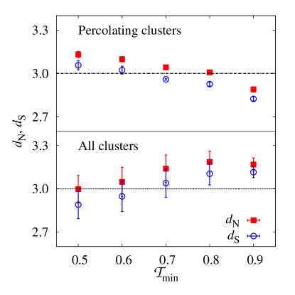
In order to proceed to a more quantitative assessment of the situation we need to go a step further. Asymptotically one expects that for large volumes $\overline{N}\propto L^{d_{N}}$, where the over-line is for the average over the quenched disorder and $d_{N}$ is the exponent that characterizes the asymptotic growth. We are ignoring here sub-leading corrections since our numerical data would not allow to fit them (we work with $L=16$, $24$ and $32$, i.e. we use three data points in each fit): also it turns out that the best fits to the simple form with the leading scaling behavior are very good, with low values of the $\chi^{2}$. Analogously we define the exponent $d_{S}$ by the rate of increase of the cluster surfaces with the volume, i.e. $\overline{S}\propto L^{d_{S}}$.

By fitting our numerical data we obtain the values of the exponents that we show in figure 2. In the case of the ferromagnetic Ising model our procedure, as applied to the magnetization-magnetization connected correlation functions, would find, for $T\neq T_{c}$, finite clusters of typical size $\xi$. We plot the values of the exponents in the two cases where we either consider all clusters, or only percolating clusters. A few comments are in order. The dependence of the exponents on the value of ${\cal T}_{{min}}$ is very weak: they both stay in the range $(2.8,3.3)$ for values of ${\cal T}_{{min}}$ ranging from $0.5$ to $0.9$. In all these cases $d_{N}$ and $d_{S}$ are very similar: their difference never exceed $0.1$. So, to summarize, both exponents turn out to be stable as a function of ${\cal T}_{{min}}$ and $\lambda$, close to the values $3$ and very close together. The low energy droplets in our system, at a value of the temperature deep in the broken phase, appear to have, as far as we can observe on the finite volume we can thermalize, a very diffused interface, compatible with being space filling (namely $d_{S}=3$).

Figure 2: The exponents $d_{S}$ and $d_{N}$ as a function of the correlation threshold ${\cal T}_{{min}}$, considering either all connected clusters (bottom) or percolating clusters only (top).

4 Sponges

In a situation where the system is non critical we expect connected clusters to have a (finite) size of the order of the correlation length: survival, in the infinite volume limit, of extended clusters is a signal of criticality. Such extended clusters can be defined, on a finite lattice, in many different ways: we will use here a very restrictive definition that we will denote by the word “sponge”[14]. We declare a connected cluster to be sponge-like if both it and at least one connected component of its complement span the whole lattice in the $x$, $y$ and $z$ directions. Only percolating clusters contribute to sponges. We use the same cutoff $\lambda=0.5$, excluding clusters that take a too large fraction of the lattice. This applies to ${\cal C}_{i}$ and to clusters in the complement of ${\cal C}_{i}$.

Figure 3:

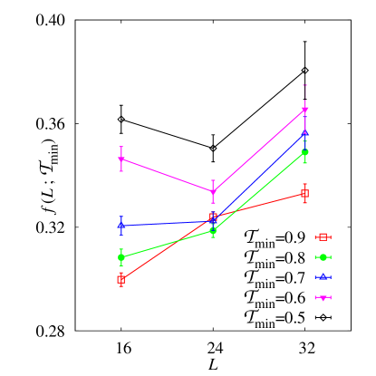
Fraction of sponges as a function of the (linear) lattice size.

We show in figure 3 the fraction of sponges as a function of the (linear) lattice size. We use different values of ${\cal T}_{{min}}$. We compute the fraction of sponges for a given disorder sample and we average this fraction over the random quenched disorder. The fraction of sponges is sizable (of order $1/3$ with the very low cutoff $\lambda=0.5$) and is never decreasing for increasing lattice size: the clear signal one gets from these numerical data is that sponges will survive in the infinite volume limit, and the typical configurations of the system will be critical. It is clear that a numerical study of this kind cannot, for many reasons, give a clear cut answer, but in the very large volume range where the Janus numerical simulations allow us to study equilibrium at low $T$ we are getting a clear hint towards survival of extended excitations (using different values of $\lambda$ would not change the picture): this is what one would expect in a situation where RSB holds. The same situation was found by analyzing ground states of the system in ref. [14]. Here we are working at finite $T<T_{c}$, with thermalized spin configuration. The two results are in some sense complementary: we are interested in a $T=0$ fixed point, so we would like to be at low $T<T_{c}$, as close to $T=0$ as possible (in principle at $T$ infinitesimally close to zero). The analysis at $T=0$ gives very interesting information, but cannot exclude the possibility that $T=0$ is a point with a special behavior.

5 Typical lengths of non-extended clusters

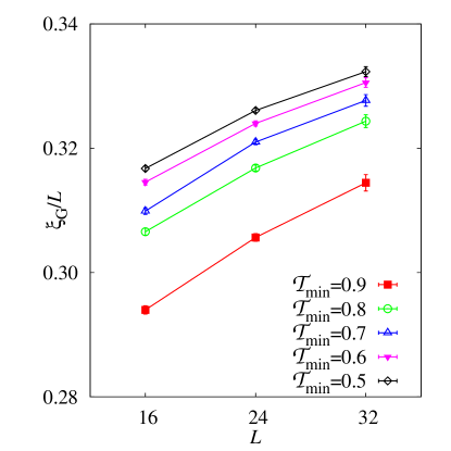
Last we investigate the geometrical structure of the connected clusters, trying to determine a typical correlation length: we summarize our results in figure 4. For each given disorder samples we only consider the clusters that do not percolate in any direction, and select the one with the largest gyration radius:

$$\xi_{G}^{(J)}\equiv\sqrt{\frac{1}{N}\sum_{k=1}^{N}r_{k}^{(2)}}\;,$$

where $r_{k}^{(2)}$ is the square distance of site $k$ from the center of mass of the cluster, and the sum runs over all sites of the cluster. For fixed $T$ and $V$ we average $\xi_{G}^{(J)}$ over all disorder samples to obtain $\xi_{G}$, that we plot, divided by $L$ in figure 4. We plot the results for different values of ${\cal T}_{{min}}$ with different symbols.

Figure 4: $\xi_{G}/L$ versus $L$. The correlation length $\xi_{G}$ is defined from the non percolating cluster with the largest radius.

Selecting the largest, non percolating cluster, allows us to pick up the largest physical length scale on a given finite lattice: the procedure is analogous to the one used in a normal ferromagnet to measure a physical, finite, correlation length below the critical point.

In a spin glass we have a critical temperature and all temperature values that are below it are possibly critical (i.e. they can have an infinite correlations length): because of this the analysis is more delicate than in a ferromagnet, We note first that the result does not depend much on ${\cal T}_{{min}}$ and $\lambda$: the emerging picture is really very stable. A constant value of $\xi_{G}/L$ would imply a divergence of the correlation length typical of a critical point: we observe indeed a slight increase of this ratio, that we attribute to finite size effects. Again, all the signatures we are detecting call for a picture where a diverging length is determining the behavior of the system. Using the non percolating cluster with the largest number of sites, instead of the one with the largest radius, does give the same kind of behavior.

6 Conclusions

We have analyzed large-scale excitations of the system, estimated critical exponents, the probability of finding large excitations, and the gyration radius as an estimator of a correlation length. We have been able to work on thermalized spin configurations at low $T$ on large lattices (experiments on spin glasses [16] show that we are working on length scales not far from the physically relevant ones).

The emerging picture is strongly suggestive of the presence of RSB (and compatible with a TNT scenario): typical excitations are large and their interface is very dense, compatible with being, in the infinite volume limit, space filling. In order to have exponents compatible with the exponents we have measured, droplets should be very different from the excitations originally proposed in the “droplet picture”

References

- [1] Mézard M, Parisi G and Virasoro M 1987 Spin Glass Theory and Beyond (Singapore: World Scientific) Fischer K H and Hertz J A 1991 Spin Glasses (Cambridge: Cambridge University Press) Young A P ed 1997 Spin Glasses and Random Fields (Singapore: World Scientific) Binder K and Kob W 2005 Glassy Materials and Disordered Solids (Singapore: World Scientific)
- [2] Parisi G 1979 Phys. Lett. 73A 203 Parisi G 1980 J. Phys. A 13 L115 Parisi G 1980 J. Phys. A 13 1101
- [3] Talagrand M 2006 Ann. Math. 163 221
- [4] McMillan W L 1984 J. Phys. C 17 3179 Fisher D S and Huse D A 1986 Phys. Rev. Lett. 56 1601 Fisher D S and Huse D A 1988 Phys. Rev. B 38 386 Bray A J and Moore M A 1987 Scaling theory of the ordered phase of spin glasses Heidelberg Colloquium on Glassy Dynamics ( Lecture Notes in Physics vol 275) ed J L van Hemmen and I Morgenstern (Berlin, Springer) p 121
- [5] Marinari E, Parisi G, Ricci-Tersenghi F, Ruiz-Lorenzo J J and Zuliani F 2000 J. Stat. Phys. 98 973
- [6] Moore M A 2005 J. Phys. A: Math. Gen. 38 L783
- [7] Krzakala F and Martin O C 2000, Phys. Rev. Lett. 85 3013 Katzgraber H G, Palassini M and Young A P 2001 Phys. Rev B 63 184422 Hartmann A K and Ricci-Tersenghi F 2002, Phys. Rev. B 66 224419
- [8] Alvarez Baños R et al, the Janus Collaboration 2010 J. Stat. Mech. P06026
- [9] Alvarez Baños R et al, the Janus Collaboration 2010 Phys. Rev. Lett. 105 177202
- [10] Billoire A, Fernandez A, Maiorano A, Marinari E, Martin-Mayor V and Yllanes D 2011 J. Stat. Mech. P10019
- [11] Alvarez-Baños R et al., the Janus Collaboration 2012 Proc. Natl. Acad. Sci. USA 109 6452
- [12] Baity-Jesi M et al., The Janus collaboration 2012 Reconfigurable computing for Monte Carlo simulations: results and prospects of the Janus project to be published on EPJST (Preprint arXiv:1204.4134)
- [13] Billoire A, Kondor I, Lukic J and Marinari E 2011 J. Stat. Mech. P02009.
- [14] See Krzakala F, Houdayer J, Marinari E, Martin O C and Parisi G 2001 Phys. Rev. Lett. 87 197204 and references therein
- [15] Geyer C J 1991 Markov chain Monte Carlo maximum likelihood, in the Proceedings of the 23rd Symposium on the Interface between Computing Science and Statistics Marinari E and Parisi G 1992 Europhys. Lett. 19 451 Geyer C J and Thompson E A 1995 J. Am. Stat. Assoc. 90 909 Tesi M C, Janse van Rensburg E C, Orlandini E and Whillington S G 1996 J. Stat. Phys. 82 155 Hukushima K and Nemoto K 1996 J. Phys. Soc. Jpn. 65 1604 Marinari E 1998 Optimized Monte Carlo Methods Advances in Computer Simulation (Lecture Notes in Physics vol 501) ed J Kertész and I Kondor (Berlin: Springer) p 50
- [16] Joh Y G, Orbach R, Wood G G, Hammann J and Vincent E 1999 Phys. Rev. Lett. 82 438