A Multivariate Graphical Stochastic Volatility Model
Abstract
The Gaussian Graphical Model (GGM) is a popular tool for incorporating sparsity into joint multivariate distributions. The G-Wishart distribution, a conjugate prior for precision matrices satisfying general GGM constraints, has now been in existence for over a decade. However, due to the lack of a direct sampler, its use has been limited in hierarchical Bayesian contexts, relegating mixing over the class of GGMs mostly to situations involving standard Gaussian likelihoods. Recent work, however, has developed methods that couple model and parameter moves, first through reversible jump methods and later by direct evaluation of conditional Bayes factors and subsequent resampling. Further, methods for avoiding prior normalizing constant calculations–a serious bottleneck and source of numerical instability–have been proposed. We review and clarify these developments and then propose a new methodology for GGM comparison that blends many recent themes. Theoretical developments and computational timing experiments reveal an algorithm that has limited computational demands and dramatically improves on computing times of existing methods. We conclude by developing a parsimonious multivariate stochastic volatility model that embeds GGM uncertainty in a larger hierarchical framework. The method is shown to be capable of adapting to the extreme swings in market volatility experienced in 2008 after the collapse of Lehman Brothers, offering considerable improvement in posterior predictive distribution calibration.
1 Introduction
The Gaussian graphical model (GGM) has received widespread consideration (see Jones et al.,, 2005) and estimators obeying graphical constraints in standard Gaussian sampling were proposed as early as Dempster, (1972). Initial incorporation of GGMs in Bayesian estimation largely focus on decomposable graphs (Dawid and Lauritzen,, 1993), since prior distributions factorize into products of Wishart distributions. Roverato, (2002) proposes a generalized extension of the Hyper-Inverse Wishart distribution for covariance matrices over arbitrary graphs. Atay-Kayis and Massam, (2005) turn this into a prior specified for precision matrices and outline a Monte Carlo (MC) method that enables pairwise model comparisons. Following Letac and Massam, (2007) and Rajaratnam et al., (2008), Lenkoski and Dobra, (2011) term this distribution the G-Wishart, and propose computational improvements to direct model comparison and model search.
A number of samplers for precision matrices under a G-Wishart distribution have been proposed. These involve either block Gibbs sampling (Piccioni,, 2000), Metropolis-Hastings (MH) moves (Mitsakakis et al.,, 2011; Dobra and Lenkoski,, 2011; Dobra et al.,, 2011), or rejection sampling (Wang and Carvalho,, 2010). Dobra et al., (2011) shows that the rejection sampler of Wang and Carvalho, (2010) suffers from extremely low acceptance probabilities in even moderate dimensions. Wang and Li, (2012) conclusively show that block Gibbs sampling is both computationally more efficient and exhibits considerably less autocorrelation than the MH methods.
The block Gibbs sampler provides a Markov chain Monte Carlo (MCMC) sample. When the likelihood assumes standard Gaussian sampling, determining posterior expectations of can technically be performed as in Lenkoski and Dobra, (2011), whereby model probabilities are first directly assessed via stochastic search, and model averaged samples are then collected using block Gibbs over each model. However, when the GGM is specified over latent data in a hierarchical Bayesian framework, such an approach is no longer valid. This is due to the use of the matrix in updating other hyperparameters as well as its involvement in updating the latent Gaussian factors.
Dobra and Lenkoski, (2011) propose a reversible jump MCMC (which for brevity we refer to as RJ) method (Green,, 1995) that simultaneously updates the GGM and its associated , and embed the GGM in a semiparametric Gaussian copula. Dobra et al., (2011) expand the RJ algorithm and show how GGMs may be used to model dependent random effects in a generalized linear model context, focusing on lattice data. Wang and Li, (2012) utilize conditional properties of G-Wishart variates that enables model moves through calculation of a conditional Bayes factor (CBF) (Dickey and Gunel,, 1978) and subsequently update through direct Gibbs sampling. Wang and Li, (2012) also explore the use of a double MH algorithm (Liang,, 2010) to avoid the computationally expensive and numerically unstable MC approximation of normalizing constants proposed by Atay-Kayis and Massam, (2005).
We investigate an alternative method for simultaneously updating the GGM and associated in hierarchical Bayesian settings. Our method is built on the framework outlined in Wang and Li, (2012), but blends several of the developments above to yield an algorithm with considerably less computational cost. We show that use of a CBF on the Cholesky decomposition of a permuted version of , originally proposed in an early version of Wang and Li, (2012), enables fast model moves; use of methods for sparse Cholesky decompositions (Rue,, 2001) further reduce computational overhead. We then show that while both Dobra et al., (2011) and Wang and Li, (2012) indicate the random walk MH sampler of Mitsakakis et al., (2011) is not suitable for posterior sampling, it is especially useful in the context of the double MH algorithm. We are therefore able to specify a model move algorithm which requires little computational effort and exhibits no numerical instability.
Simulation experiments compare our new algorithm to the algorithm of Wang and Li, (2012) (which we refer to as WL). Both methods perform equally well at determining posterior distributions. However, we show that while the WL approach is theoretically appealing, it suffers significant computational overhead on account of many matrix inversions. By contrast, our new approach exhibits a dramatic improvement in computation time.
We conclude with an example of how GGMs may be embedded in hierarchical Bayesian models. GGMs have been shown to yield parsimonious joint distributions useful in financial applications (Carvalho and West,, 2007; Rodriguez et al.,, 2011). However, existing studies have largely ignored heteroskedasticity in financial data and relied on datasets taken over periods with relatively little financial turmoil. To address this, we propose a parsimonious multivariate stochastic volatility model that incorporates GGM uncertainty. We then model stock returns for assets during the period surrounding the financial crash of 2008. We show that in the periods leading up to the crash, and 9 months after the most turbulent period, this method yields no improvement over an approach that does not model heteroskedasticity. However, during the period of heightened volatility, our new model is able to adapt quickly and yields considerably more calibrated predictive distributions.
The article is organized as follows. In Section 2 we review the G-Wishart distribution, establish results necessary for CBF calculations and describe the block Gibbs sampler. Section 3 conducts a simulation study showing the computational advantage gained by our new algorithm. In Section 4 we describe our multivariate graphical stochastic volatility model and give results over the data mentioned above. We conclude in Section 5.
2 The G-Wishart Distribution
2.1 Review of Basic G-Wishart Properties
Suppose that we collect data such that independently for , where , the space of positive definite matrices. This sample has likelihood
where denotes the trace inner product and .
Further suppose that is a GGM where and . We will slightly abuse notation throughout, by writing to indicate that the edge is in the edge set . Associated with is a subspace such that implies that and whenever . The G-Wishart distribution (Roverato,, 2002; Atay-Kayis and Massam,, 2005) assigns prior probability to as
The normalizing constant is in general not known to have an explicit form, and Atay-Kayis and Massam, (2005) propose an MC approximation for this factor. Furthermore, the G-Wishart is conjugate and thus where .
Let be the upper triangular matrix such that , the Cholesky decomposition. Rue, (2001) notes that we may associate with another graph , called the fill-in graph, such that , when and
| (1) |
when and . Rue, (2001) outlines a straightforward method for constructing a graph from and explains how use of node reordering software can minimize fill-in.
Roverato, (2002) shows that if then
| (2) |
where is number of nodes in that are connected to node in . We especially note that if , then
| (3) |
2.2 Sampling Methods
We review two MCMC methods for approximate sampling from a . See Dobra et al., (2011) and Wang and Li, (2012) for more detailed reviews of the many methods that have been proposed.
Let denote the cliques of . In the following, we consider a clique to be a maximally complete subgraph, though Wang and Li, (2012) note that this can be relaxed to any complete subgraph. Piccioni, (2000) shows that for any ,
| (4) |
where denotes a standard Wishart variate. The expression (4) thereby gives the full conditionals of . The block Gibbs sampler thus cycles through , updating each component using (4). Wang and Li, (2012) convincingly show that for posterior inference of the block Gibbs sampler outperforms all other proposed methods, both in terms of computing time and mixing. The authors also provide a useful review of the algorithm and indicate its broad flexibility. Throughout, we use the block Gibbs sampler for updating the matrix in the posterior.
Both Dobra et al., (2011) and Wang and Li, (2012) show that the random walk MH (RWMH) algorithm of Mitsakakis et al., (2011) is unsuitable for posterior inference. However, we show below that it is especially effective to use in the double MH algorithm. In particular, suppose that we wish to sample from and is the current state of an MCMC chain. Then the RWMH algorithm performs the following
-
1.
Determine from
-
2.
Propose :
-
a.
Sample and set
-
b.
Sample for
-
c.
Complete using (1) for all
-
a.
-
3.
Compute
(5) -
4.
With probability set
The appeal of the RWMH algorithm in sampling from is the simplicity of the factor in (5). Through the use of node reordering software, which minimizes the size of , this expression may require few calculations. While the algorithm does not perform well in the posterior, and the calculation as well as step (2.c) become more involved when we show below that in the particular case of the double MH algorithm using the prior , this method is extremely useful.
2.3 Conditional Bayes Factors
Prior to Wang and Li, (2012), model moves between two graphs and focused on approximating the ratio
| (6) |
first through MC (Atay-Kayis and Massam,, 2005; Jones et al.,, 2005), then a combination of MC and Laplace approximation (Lenkoski and Dobra,, 2011) and ultimately through RJ (Dobra and Lenkoski,, 2011; Dobra et al.,, 2011).
Suppose that which differ only by the edge and that . Let . In lieu of (6), Wang and Li, (2012) consider ratios of the form
| (7) |
which are related to the conditional Bayes factors (CBFs) of Dickey and Gunel, (1978).
Using properties related to the form (4) Wang and Li, (2012) show that
| (8) |
where, in general
where ,
such that . The matrix is equal to except that and . Finally, the matrix is equal to except that .
By using the CBF in (8), Wang and Li, (2012) propose model moves that do not rely on RJ methods, and after assessing which graph to move to, the parameter , as well as if is in the accepted graph, are resampled according to their conditional distributions given . This method is appealing, as it offers an automatic manner of moving between graphs and does not rely on the tuning parameters used in the RJ methods of Dobra and Lenkoski, (2011) and Dobra et al., (2011).
While the result has significant theoretical appeal we show that computation of the factor is extremely costly, even in low dimensions. This is due to the formation of the matrices and , which require the solution of systems involving large matrices, in particular, and .
Suppose now that and differ only by the edge again with . We consider the CBF
where . In Appendix A we show that
| (9) |
with, in general
where , and .
This result originally appeared in an early version of Wang and Li, (2012). In order to update a general edge , we propose determining a permutation of such that the nodes of are reordered to reduce the fill-in of the graph and finally, the edge is placed in the position. Equation (9) is then calculated after permuting, and according to .
The benefit of this method is the reduced computational overhead required to compute (9). The method requires relabeling the matrices and and determining the Cholesky decomposition of the permuted version of . Using node reordering software to minimize fill-in of proves useful in the developments below.
2.4 Avoiding Normalizing Constant Calculation
Both (8) and (9) require determination of the prior normalizing constants and . While the MC method of Atay-Kayis and Massam, (2005) enables these factors to be approximated, the routine can be subject to numerical instability (Lenkoski and Dobra,, 2011; Wang and Li,, 2012) and involves significant computational effort.
Wang and Li, (2012) propose a method for avoiding the use of the MC approximation for prior normalizing constants. Their method employs the double Metropolis Hastings algorithm of Liang, (2010), which is an extension of the exchange algorithm developed by Murray et al., (2006).
We briefly review the implementation of the double MH algorithm in Wang and Li, (2012). Suppose that is the current state of the MCMC chain and we propose to move to by adding the edge to . The double MH algorithm then forms a copy of , resamples and according to . It then updates via block Gibbs according to . Equation (8) is then replaced with
| (10) |
We see that the expression (10) has replaced the prior normalizing constants with an evaluation of in the prior, evaluated at (see Murray et al.,, 2006; Liang,, 2010, for theoretical justifications of this procedure). This is clearly beneficial, as it avoids the need for involved MC approximation. Unfortunately, the procedure as implemented in Wang and Li, (2012) requires a full run of the block Gibbs sampler, as well as determination of the matrices and and therefore contains many large matrix operations.
We propose an alternative implementation of the double MH algorithm. Again suppose that is the current state and we propose to move to by adding the edge . We first determine from . We then update to using the RWMH algorithm in Section 2.2 relative to . Equation (9) is then replaced with
| (11) |
We can immediately see that the expression (11) is considerably simpler that (10); it requires no additional matrix inversions nor the evaluation of any trace inner products. Furthermore, the generation of the auxiliary variables through the RWMH is considerably less demanding computationally than the use of the Block Gibbs sampler, especially when , a common setting in practice.
2.5 Algorithms for Full Posterior Determination
In this section we outline the two algorithms we will consider for full posterior determination. Both algorithms create a sequence where . Given the current state the WL algorithm proceeds as follows
-
0.
Set and
-
1.
For each edge , do:
-
a.
if attempt to update to with probability
if the ratio is flipped. If is not to be updated, skip to step c.
-
b.
If attempting to update to , sample as discussed in Section 2.4 and calculate
if , otherwise calculate
and with probability set , otherwise leave it unchanged.
-
c.
Resample according to .
After attempting to update each edge, set .
-
a.
-
2.
Resample using the block Gibbs sampler relative to and the current state of .
We see that in one iteration of the WL algorithm, each edge is potentially updated in the graph. Our new algorithm (which we call CL) also follows this idea, and proceeds as follows
-
0.
Set and
-
1.
For each edge , do:
-
a.
Determine a permutation of as discussed in Section 2.3, which places the edge in the position, and likewise permute , , and . Let denote the permuted version of and be the Cholesky decomposition of the permuted version of . If attempt to update to with probability
if the ratio is flipped. If is not to be updated then, skip to step c.
-
b.
If attempting to update to , sample as discussed in Section 2.4 and calculate
if , otherwise calculate
and with probability set , otherwise leave it unchanged.
-
c.
Resample according to . Then reform and by unpermuting the system.
After attempting to update each edge, set .
-
a.
-
2.
Resample using the block Gibbs sampler relative to and the current state of .
As we can see, there is somewhat more bookkeeping involved in the implementation of the CL algorithm, as the system is constantly being permuted. However, the reduction in computation time by using the RWMH algorithm and requiring only the calculation of the factors and is dramatic, as we show below.
3 Simulation Study
In this section we conduct a simulation study that compares the method we have developed to the WL algorithm. Our example comes directly from Wang and Li, (2012). We consider a situation in which and let where and for for and . We finally assume the prior . Using exhaustive MC approximation of the entire graph space, Wang and Li, (2012) show that the posterior probability of each edge is
We use this example and compare the CL algorithm to the WL algorithm. Following Wang and Li, (2012) we run both the WL and CL algorithms as described in Section 2.5 for iterations and discard the first iterations as burn-in. Both algorithms were implemented in R, though C++ was used for block-Gibbs updates. We note that if a pure R implementation had been used, the time differences between WL and CL would be even more dramatic.
We record the total computing time and looked at the mean squared errors of the posterior inclusion probabilities from the two runs compared with the true values given above. We repeated the entire process times, each time starting both WL and CL from the same random starting point. Table 1 shows the average computing time in seconds (on a 2.8 GHz desktop computer with 4GB of RAM running Linux), average MSE and standard deviations across the runs. The first column shows the expected result: even in six dimensions the WL algorithm takes more than 4 times as long to perform the same number of iterations as the CL algorithm. This shows the improved efficiency of the proposed method.
| Time (sec) | MSE | |||
|---|---|---|---|---|
| Mean | SD | Mean | SD | |
| CL | 182.5 | (4.1) | 0.0088 | (6e-04) |
| WL | 818.4 | (19.2) | 0.0349 | (0.0025) |
We found the results in the third column surprising, but do not draw broad conclusions from it. It appears that in this example, using iterations, the CL algorithm approaches the true posterior edge expectation more quickly than the WL algorithm. Since both algorithms are correct theoretically, we choose not to emphasize this result. Furthermore, we have determined that by doubling the number of iterations, both approaches yield essentially the exact posterior distribution, though again the WL algorithm takes more than 4 times as long to run.
This example was chosen as it appears in Wang and Li, (2012) and has an exact answer. The fact that the CL algorithm is considerably faster than the WL approach even in 6-dimensions indicates the broader appeal for searching truly high dimensional spaces.
4 A Multivariate Graphical Stochastic Volatility Model
Modeling the joint distribution of returns for a large number of assets is an important component of portfolio allocation and risk management. Carvalho and West, (2007) and Rodriguez et al., (2011) both show that the use of GGMs can substantially improve modeling of joint asset returns. However, heterogeneity in asset returns was, at best, tangentially addressed. The study of Carvalho and West, (2007) considered a fixed (decomposable) graph throughout the entire period and assumed that asset returns were identically distributed. Rodriguez et al., (2011) allowed for mixing over the class of decomposable graphs and also introduced some heterosckedasticity by considering an infinite-dimensional hidden Markov model (iHMM). However, inside groups of observations in the iHMM, variances were assumed constant.
Despite these constraints in model assumptions, both studies showed substantial improvements by incorporating GGMs into the precision matrix associated with joint asset returns. We consider a situation in which the notion of homoskedastic, normally distributed asset returns is simply untenable; namely, the period surrounding the financial turbulence associated with the collapse of Lehman Brothers. We show that by utilizing the developments in the previous sections, we are able to specify a parsimonious stochastic volatility model for multivariate assset returns that quickly adapts to changes in market volatility. This model shows the flexibility of the new approach in embedding the GGM in larger hierarchical Bayesian frameworks.
4.1 The stochastic volatility model
Let be the log-returns of correlated assets. We specify the following hierarchical model for these returns
| (12) | ||||
In the likelihood (12) we see that asset returns are assumed to be mean-zero. The terms then dictate an overall level of market volatility, while a constant precision parameter dictates the degree to which asset returns are correlated. While this model is parsimonious, it serves as a useful first departure from previous studies as it explicitly incorporates notions of stochastic volatility. For purposes of identification, we set . In the conclusions section we discuss further possible generalizations to this framework.
After collecting a time-series of returns , we then aim to determine the posterior distribution
where . Furthermore, we may be interested in the posterior predictive distribution . The parameters are updated with standard block MH or Gibbs steps (see Rue and Held,, 2005) and the posterior predictive distribution is easily formed from these parameters. However, we note in particular that
| (13) |
From (13) we see why the developments in Section 2 prove useful. We may update and jointly using the CL algorithm discussed in Section 2.5 simply by setting . This allows us to easily embed a sparse precision matrix and mix over the class of GGMs in any hierarhical Bayesian model that involves a standard Wishart distribution.
4.2 The data
To apply our model and algorithm we randomly chose 20 stocks from the
S&P 500. These stocks were: Aetna Inc. (AET), CA Inc. (CA), Campbell Soup (CPB), CVS Caremark Corp. (CVS), Family Dollar Stores (FDO), Honeywell Int’l Inc. (HON),
Hudson City Bancorp (HCBK), JDS Uniphase Corp. (JDSU), Johnson Controls (JCI), Morgan Stanley (MS), PPG Industries (PPG),
Principal Financial Group (PFG), Sara Lee Corp. (SLE), Sempra Energy (SRE), Southern Co. (SO), Supervalu Inc. (SVU), Thermo Fisher Scientific (TMO),
Wal-Mart Stores (WMT), Walt Disney Co. (DIS), Wellpoint Inc. (WLP).
We chose a time period where markets experience both high and low volatility to evaluate the flexibility of our model. We chose the time
period from October 31, 2001 to May 21, 2008 as our training period to
fit our model and make predictions for the time period from May
22, 2008 to October 23, 2009. The time periods consist of 1650 and 360
trading days respectively. Figure 1 shows the mean of the squared returns for the these 20 securities over the entire dataset. The extreme volatility present in the markets after the collapse of Lehman brothers in September 2008 is readily evident, showing that a homoskedasticity assumption is untenable for these data.

4.3 Predictive Performance Results
We assess the relative performance of the stochastic volatility model we develop in Section 4.1 versus a method that embedds GGMs, but does not have a stochastic volatility component. For each day in the forecast period we run our stochastic
volatility model from the beginning of the training period
until the previous day
to obtain estimates for the model parameters. We run the algorithm for iterations, discarding the first as burn-in (keep in mind that in one iteration of the algorithm all edges are evaluated). Using the posterior sample, we obtain the posterior predictive distribution of .
Figure 2 shows the mean of the posterior predictive distribution of the volatility component using the returns up to time , which drives the predictive distribution of for each day in the forecast period. Comparing Figures 1 and 2 we see
that our model reflects the time-dependent volatility well. At the beginning when the market is quiet, takes lower values mostly between 0 and 1. After the shock of the financial crisis the
volatility in the market goes up extremely, which is reflected by significantly higher values of . Months later, towards the end of the forecast period, the market has cooled down and the terms reflect this.

The two methods we compare both return full predictive distributions. By construction, these predictive distributions have the same mean and median since returns are assumed mean-zero. Judging their performance therefore requires assessing the entire predictive distribution. We assess their performance using the energy score introduced by Gneiting and Raftery, (2007).
The energy score is a proper scoring rule, which is a multivariate
generalization of the continuous ranked probability score. It is defined as
| (14) |
where is our predictive distribution for a vector-valued quantity,
and are independent random variables with
distribution and
is the realization.
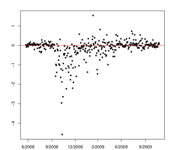
For each day in the forecast period, we compute the energy score for the predictive distribution returned by the two methods considered. Figure 3 shows the difference between the stochastic volatility model developed in Section 4.1 and the model that incorporates GGM uncertainty but holds volatility fixed. As we can see in Figure 3, between May and August, 2008, there is no clear difference between the two approaches. However, after the financial turbulence in September, 2008, the stochastic volatility model outperforms the fixed volatility model by a considerable margin. During almost every day in the turbulent period, the energy scores are lower under the stochastic volatility model. After the market turbulence subsides, the two models return to performing equally well again.
This short example shows the utility of the computational methodology developed in this paper. The model is simple, in many respects, but a non-trivial deviation from the standard iid sampling framework to which the GGM was initially relegated. By now being able to embed the GGM in more complicated hierarchical frameworks, we are able to address difficult sampling schemes while simultaneously incorporating sparsity in the estimate of joint distributions.
5 Conclusions
We have synthesized a number of recent results related to the G-Wishart distribution. This has allowed for an algorithm that does not rely on RJ methods, obviates the need for expensive and numerically unstable MC approximation of prior normalizing constants and does so with minimal computational effort. The improvement in computation time is sufficient that at each stage of the algorithm, all edges may be evaluated for inclusion or exclusion in the graphical model. This algorithm allows the GGM to be embedded in more sophisticated hierarchical Bayesian models and opens the possibility of replacing standard Wishart distributions with G-Wishart variates, leveraging the improvement in predictive performance offered by sparse precision matrices.
The applied example shows the usefulness of this combination. We are able to sparsely model the interactions in financial assets while simultaneously addressing the issues of stochastic volatility prevalent in markets undergoing turbulence. The method is able to characterize the distribution of asset returns during periods of rapidly fluctuating volatility much better than standard iid frameworks.
The stochastic volatility model we develop remains parsimonious and several adjustments could be made. The first such development would be to replace the univariate term with a multivariate factor that allows the variance of each asset to follow its own path, while potentially tying the evolution of these factors together with a separate GGM. Furthermore, employing some form of the iHMM framework of Rodriguez et al., (2011) could allow for the matrix to change throughout the period as well. Such developments will be considered in future work.
References
- Atay-Kayis and Massam, (2005) Atay-Kayis, A. and Massam, H. (2005). A Monte Carlo method for computing the marginal likelihood in nondecomposable Gaussian graphical models. Biometrika, 92:317–335.
- Carvalho and West, (2007) Carvalho, C. M. and West, M. (2007). Dynamic matrix-variate graphical models. Bayesian Analysis, 2:69–98.
- Dawid and Lauritzen, (1993) Dawid, A. P. and Lauritzen, S. L. (1993). Hyper Markov laws in the statistical analysis of decomposable graphical models. Ann. Statist., 21:1272–1317.
- Dempster, (1972) Dempster, A. P. (1972). Covariance selection. Biometrics, 28:157–175.
- Dickey and Gunel, (1978) Dickey, J. M. and Gunel, E. (1978). Bayes factors from mixed probabilities. J. R. Statist. Soc. B, 40:43–46.
- Dobra and Lenkoski, (2011) Dobra, A. and Lenkoski, A. (2011). Copula gaussian graphical models and their application to modeling functional disability data. Annals of Applied Statistics, 5:969–993.
- Dobra et al., (2011) Dobra, A., Lenkoski, A., and Rodriguez, A. (2011). Bayesian inference for general gaussian graphical models with application to multivariate lattice data. Journal of the American Statistical Association, Forthcoming.
- Gneiting and Raftery, (2007) Gneiting, T. and Raftery, A. E. (2007). Strictly proper scoring rules, prediction and estimation. Journal of the American Statistical Association, 102:359–378.
- Green, (1995) Green, P. J. (1995). Reversible jump Markov chain Monte Carlo computation and Bayesian model determination. Biometrika, 82(711-732).
- Jones et al., (2005) Jones, B., Carvalho, C., Dobra, A., Hans, C., Carter, C., and West, M. (2005). Experiments in stochastic computation for high-dimensional graphical models. Statistical Science, 20:388–400.
- Lenkoski and Dobra, (2011) Lenkoski, A. and Dobra, A. (2011). Computational aspects related to inference in Gaussian graphical models with the G-Wishart prior. Journal of Computational and Graphical Statistics, 20:140–157.
- Letac and Massam, (2007) Letac, G. and Massam, H. (2007). Wishart distributions for decomposable graphs. Ann. Statist., 35:1278–323.
- Liang, (2010) Liang, F. (2010). A double Metropolis-Hastings sampler for spatial models with intractable normalizing constants. Journal of Statistical Computing and Simulation, 80:1007–1022.
- Mitsakakis et al., (2011) Mitsakakis, N., Massam, H., and Escobar, M. D. (2011). A Metropolis-Hastings based method for sampling from the g-Wishart distribution in Gaussian graphical models. Electronic Journal of Statistics, 5:18–30.
- Murray et al., (2006) Murray, I., Ghahramani, Z., and MacKay, D. (2006). Mcmc for doubly-intractable distributions. Proceedings of the 22nd Annual Conference on Uncertainty in Artificial Intelligence.
- Piccioni, (2000) Piccioni, M. (2000). Independence structure of natural conjugate densities to exponential families and the Gibbs Sampler. Scand. J. Statist., 27:111–27.
- Rajaratnam et al., (2008) Rajaratnam, B., Massam, H., and Carvalho, C. M. (2008). Flexible covariance estimation in graphical Gaussian models. Ann. Statist., 36:2818–2849.
- Rodriguez et al., (2011) Rodriguez, A., Dobra, A., and Lenkoski, A. (2011). Sparse covariance estimation in heterogeneous samples. Electronic Journal of Statistics, 5:981–1014.
- Roverato, (2002) Roverato, A. (2002). Hyper inverse Wishart distribution for non-decomposable graphs and its application to Bayesian inference for Gaussian graphical models. Scand. J. Statist., 29:391–411.
- Rue, (2001) Rue, H. (2001). Fast sampling of Gaussian Markov random fields. Journal of the Royal Statistical Society, Series B, 63:325–338.
- Rue and Held, (2005) Rue, H. and Held, L. (2005). Gaussian Markov Random Fields. Chapman & Hall.
- Wang and Carvalho, (2010) Wang, H. and Carvalho, C. M. (2010). Simulation of hyper-inverse Wishart distributions for non-decomposable graphs. Electronic Journal of Statistics, 4:1470–1475.
- Wang and Li, (2012) Wang, H. and Li, S. Z. (2012). Efficient Gaussian graphical model determination under g-wishart prior distributions. Electronic Journal of Statistics, 6:168–198.
Appendix A: Determination of CBF for using
Consider
we note that
and
up to common terms we thus have that
recognizing the integral as the kernel of a normal distribution, this yields
Further, again up to common terms
and thus