Form factors of radiative pion decays in nonlocal chiral quark models

Abstract

We study the radiative pion decay $\pi^{+}\rightarrow e^{+}\nu_{e}\gamma$ within nonlocal chiral quark models that include wave function renormalization. In this framework we analyze the momentum dependence of the vector form factor $F_{V}(q^{2})$, and the slope of the axial-vector form factor $F_{A}(q^{2})$ at threshold. Our results are compared with available experimental information and with the predictions given by the NJL model. In addition we calculate the low energy constants $\ell_{5}$ and $\ell_{6}$, comparing our results with the values obtained in chiral perturbation theory.

I Introduction

The radiative pion decay $\pi^{+}\rightarrow e^{+}\nu_{e}\gamma$ is a very interesting process from different points of view. According to the standard description, the corresponding decay amplitude consists of the inner bremsstrahlung (IB) and structure-dependent (SD) terms. The former can be associated with the diagrams in which the photon is radiated by the electrically charged external legs (either pion or lepton), while the SD terms correspond to the photon emission from intermediate states generated by strong interactions. Since the IB contribution turns out to be helicity suppressed, this process is an adequate channel to study the SD amplitude, which provides information about strong interactions in the nonperturbative regime.

The SD contribution can be parameterized through the introduction of vector and axial-vector form factors, $F_{V}(q^{2})$ and $F_{A}(q^{2})$ respectively, where $q^{2}$ is the squared invariant mass of the $e^{+}\nu_{e}$ pair Bryman:1982et . From the experimental point of view, recent analyses Bychkov:2008ws of $\pi^{+}\rightarrow e^{+}\nu_{e}\gamma$ decays have allowed the measurement of $F_{V}(0)$, $F_{A}(0)$, and the slope of the form factor $F_{V}(q^{2})$ at $q^{2}=0$. In addition, ongoing experiments are expected to reach enough statistics to determine the slope of $F_{A}(q^{2})$ at $q^{2}=0$ in the near future. On the theoretical side, the analysis of the form factors has been carried out in the framework of Chiral Perturbation Theory ($\chi$PT) Hol86 and effective meson Lagrangian methods Mateu:2007tr , which provide a good description of low-energy meson phenomenology. However, one can also address the question of how the form factors are connected to the underlying quark structure. Due to the nonperturbative nature of the quark-gluon interactions in the low-energy domain, to address this issue one is forced to deal with models that treat quark interactions in some effective way. In this sense, the widely studied Nambu–Jona-Lasinio (NJL) model is the most popular schematic quark effective theory for QCD Vogl:1991qt ; Klevansky:1992qe ; Hatsuda:1994pi . In this model quarks interact through a local, chiral invariant four-fermion coupling. Now, as a step towards a more adequate description of QCD, some extensions of the NJL that include nonlocal interactions have been proposed in the literature (see Ref. Rip97 and references therein). In fact, nonlocality arises as a natural feature of several well established approaches to low energy quark dynamics, such as the instanton liquid model SS98 , the Schwinger-Dyson resummation techniques Roberts:1994dr , and also lattice QCD calculations Parappilly:2005ei ; Bowman2003 ; Furui:2006ks . In the last years nonlocal chiral quark models have been applied to study different hadron observables with significant success Bowler:1994ir ; Scarpettini:2003fj ; GomezDumm:2006vz ; Golli:1998rf ; Rezaeian:2004nf ; Praszalowicz:2001wy ; Noguera ; Noguera:2005cc ; Noguera:2008 .

In a previous work Dumm:2010hh we have addressed the analysis of the vector and axial-vector form factors in $\pi^{+}\rightarrow e^{+}\nu_{e}\gamma$ in the framework of nonlocal chiral quark models. We have determined the values of $F_{V}(0)$, $F_{A}(0)$ and the slope of $F_{V}(q^{2})$ at $q^{2}=0$ for different parameterization sets, comparing the results with the experimental measurements and the corresponding values obtained in the NJL model. In this paper we extend these previous results, analyzing the vector form factor for values of $q^{2}$ up to 1 GeV², and studying the slope of $F_{A}(q^{2})$ at threshold. While the latter is interesting in view of the comparison with future experimental results, the study of the behavior of $F_{V}(q^{2})$ presents relevant theoretical motivations. In fact, in the isospin limit, and assuming the conserved-vector-current (CVC) hypothesis, the vector form factor can be directly related to the form factor $F^{\pi\gamma\gamma^{\ast}}(q^{2})$ associated with the vertex $\pi\gamma\gamma^{\ast}$, where $q^{2}$ is the photon virtuality in Euclidean space. Thus our results can be compared with the experimental information on $F^{\pi\gamma\gamma^{\ast}}(q^{2})$, taken e.g. from processes as $\pi^{-}p\to\pi^{0}n$ or $e^{+}e^{-}\to e^{+}e^{-}\pi^{0}$, and the compatibility with the usually assumed single-pole behavior can be analyzed. The CVC hypothesis is supported by the measured value of $F_{V}(0)$, which turns out to be fully consistent with the corresponding value taken from $F^{\pi\gamma\gamma^{\ast}}(q^{2})$ at $q^{2}=0$ pdg . We notice that the calculation of $F_{V}(q^{2})$ in the framework of nonlocal models turns out to be technically involved, due to the presence of poles and cuts arising from the dressed quark propagators. Finally, to complete our analysis we also study the compatibility of our nonlocal models with effective meson theories such as $\chi$PT. In fact, it is seen that $F_{A}(0)$ and the pion charge radius $\langle r^{2}\rangle_{\pi}$ are related to the so-called $\chi$PT low energy constants (LECs) $\ell_{5}$ and $\ell_{6}$, which encode the information of quark and gluon degrees of freedom. In $\chi$PT these LECs are input parameters taken from phenomenology, thus the compatibility with the predictions arising from effective quark models is a measure of the ability of these models to account for the underlying strong interaction physics.

The article is organized as follows: in Sect. II we describe the models and quote the analytical results for the vector form factor $F_{V}(q^{2})$. The numerical results for vector and axial-vector form factors are presented and discussed in Sect. III. In Sect. IV we quote the values for the LECs obtained within our models, while in Sect. V we present our conclusions. The full analytical expressions for the axial-vector form factor are quoted in Appendix I.

II Formalism

The amplitude for the process $\pi^{+}\rightarrow e^{+}\nu_{e}(q)+\gamma(k)$ in Minkowski space can be written as Bryman:1982et

$$\mathcal{M} =\frac{G_{F}}{\sqrt{2}}\ e\,\cos\theta_{C}\;\varepsilon^{\mu}\left[\sqrt{2}\;f_{\pi}\left\{(q+k)^{\alpha}\,L_{\alpha\mu}\;-\;l^{\nu}\left[g_{\mu\nu}\;+\;\frac{q_{\mu}q_{\nu}}{(q\cdot k)}\right]\right\}\right.$$

$$\left.\qquad\qquad\qquad+l^{\nu}\left\{-\,i\,\epsilon_{\mu\nu\alpha\beta}\;k^{\alpha}q^{\beta}\;\frac{F_{V}(q^{2})}{m_{\pi}}\;+\left[q_{\mu}k_{\nu}\;-\;g_{\mu\nu}\,(q\cdot k)\right]\frac{F_{A}(q^{2})}{m_{\pi}}\right\}\ \right]\ ,$$ (1)

with $(q+k)^{2}=m_{\pi}^{2}$, $k^{2}=0$. Here $G_{F}$ and $\theta_{C}$ stand for the Fermi constant and the Cabibbo angle, respectively; $\varepsilon_{\mu}$ is the photon polarization vector, $l_{\mu}$ is the lepton current, $L_{\alpha\mu}$ is a lepton tensor, and $F_{V}(q^{2})$ and $F_{A}(q^{2})$ denote the vector and axial-vector hadronic form factors mentioned in the Introduction. In this work we are interested in the study of these form factors in the context of nonlocal SU(2) chiral models that include wave function renormalization. These models are defined by the following Euclidean action Noguera ; Noguera:2008 :

$$S_{E}=\int d^{4}x\ \left\{\bar{\psi}(x)\left(-i\hbox to0.0pt{/\hss}\partial+m_{c}\right)\psi(x)-\frac{G_{S}}{2}\Big{[}j_{a}(x)j_{a}(x)+j_{P}(x)j_{P}(x)\Big{]}\right\}\ .$$ (2)

Here $m_{c}$ is the current quark mass, which is assumed to be equal for $u$ and $d$ quarks, while the nonlocal currents $j_{a}(x),j_{P}(x)$ are given by

$$j_{a}(x) =\int d^{4}z\ g(z)\ \bar{\psi}\left(x+\frac{z}{2}\right)\ \Gamma_{a}\ \psi\left(x-\frac{z}{2}\right)\ ,$$

$$j_{P}(x) =\int d^{4}z\ f(z)\ \bar{\psi}\left(x+\frac{z}{2}\right)\ \frac{i{\overleftrightarrow{\hbox to0.0pt{/\hss}\partial}}}{2\ \varkappa_{p}}\ \psi\left(x-\frac{z}{2}\right)\ ,$$ (3)

where $\Gamma_{a}=(\leavevmode\hbox{\small 1\kern-3.8pt\normalsize 1},i\gamma_{5}\vec{\tau})$ and $u(x^{\prime}){\overleftrightarrow{\partial}}v(x)=u(x^{\prime})\partial_{x}v(x)-\partial_{x^{\prime}}u(x^{\prime})v(x)$. The functions $g(z)$ and $f(z)$ in Eq. (3) are nonlocal covariant vertex form factors characterizing the corresponding interactions. In what follows it is convenient to Fourier transform $g(z)$ and $f(z)$ into momentum space. Note that Lorentz invariance implies that the corresponding Fourier transforms, $g_{p}$ and $f_{p}$, can only be functions of $p^{2}$.

In order to deal with meson degrees of freedom, one can perform a standard bosonization of the theory. This is done by considering the corresponding partition function $\mathcal{Z}=\int\mathcal{D}\bar{\psi}\,\mathcal{D}\psi\,\exp[-S_{E}]$, and introducing auxiliary fields $\sigma_{1}(x),\sigma_{2}(x),\vec{\pi}(x)$, where $\sigma_{1,2}(x)$ and $\vec{\pi}(x)$ are scalar and pseudoscalar mesons, respectively. An effective bosonized action is obtained once the fermion fields are integrated out. To treat that bosonic action we assume, as customary, that $\sigma_{1,2}$ fields have nontrivial translational invariant mean field values, while the mean field values of pseudoscalar fields $\pi_{i}$ are zero. Thus we write

$$\sigma_{1}(x)=\bar{\sigma}_{1}+\delta\sigma_{1}(x)\ ,\qquad\sigma_{2}(x)=\varkappa_{p}\ \bar{\sigma}_{2}+\delta\sigma_{2}(x)\ ,\qquad\vec{\pi}(x)=\delta\vec{\pi}(x)\ .$$ (4)

Replacing in the bosonized effective action and expanding in powers of meson fluctuations we get

$$S_{E}^{\mathrm{bos}}\ =\ S_{E}^{\mathrm{MFA}}\ +\ S_{E}^{\mathrm{quad}}\ +\ ...$$ (5)

Here the mean field action per unit volume reads

$$\frac{S_{E}^{\mathrm{MFA}}}{V^{(4)}}=\frac{1}{2G_{S}}\left(\bar{\sigma}_{1}^{2}+\varkappa_{p}^{2}\ \bar{\sigma}_{2}^{2}\right)-4N_{c}\int\frac{d^{4}p}{(2\pi)^{4}}\ \ln\left[\frac{z_{p}}{-\hbox to0.0pt{/\hss}p+m_{p}}\right]^{-1}\ ,$$ (6)

with

$$z_{p}=\left(1-\bar{\sigma}_{2}\ f_{p}\right)^{-1}\ ,\qquad m_{p}=z_{p}\left(m_{c}+\bar{\sigma}_{1}\ g_{p}\right)\ .$$ (7)

The minimization of $S_{E}^{\mathrm{MFA}}$ with respect to $\bar{\sigma}_{1,2}$ leads to the corresponding “gap equations”. The quadratic terms in Eq. (5) can be written as

$$S_{E}^{\mathrm{quad}}=\frac{1}{2}\int\frac{d^{4}p}{(2\pi)^{4}}\sum_{M=\sigma,\sigma^{\prime},\pi}G_{M}(p^{2})\ \delta M(p)\ \delta M(-p)\ ,$$ (8)

where $\sigma$ and $\sigma^{\prime}$ fields are scalar meson mass eigenstates, defined in such a way that there is no $\sigma-\sigma^{\prime}$ mixing at the level of the quadratic action. The explicit expressions of $G_{M}(p^{2})$, as well as those of the gap equations mentioned above, can be found in Ref. Noguera:2008 . Meson masses can be obtained by solving the equations $G_{M}(-m_{M}^{2})=0$, while on-shell meson-quark coupling constants $G_{Mq\bar{q}}$ are given by

$$\left(G_{Mq\bar{q}}\right)^{-2}=\ \frac{dG_{M}(p^{2})}{dp^{2}}\bigg{|}_{p^{2}=-m_{M}^{2}}\ .$$ (9)

As in Ref. Noguera:2008 , we will consider here different functional dependencies for the vertex form factors $g_{p}$ and $f_{p}$. First, we consider a relatively simple case in which there is no wave function renormalization of the quark propagator, i.e. $f_{p}=0$, $z_{p}$ = 1, and we take an often used exponential parameterization for $g_{p}$,

$$g_{p}=\mbox{exp}\left(-p^{2}/\Lambda_{0}^{2}\right)\ .$$ (10)

The model parameters $m_{c}$, $G_{S}$ and $\Lambda_{0}$ are determined by fitting the pion mass and decay constant to their empirical values $m_{\pi}=139$ MeV and $f_{\pi}=92.4$ MeV, and fixing the chiral condensate to the phenomenologically acceptable value $\langle\bar{q}q\rangle^{1/3}=-240$ MeV. In what follows we refer to this choice of model parameters as set A. Second, we consider a more general case that includes the $j_{P}(x)j_{P}(x)$ interaction, i.e. we consider a nonzero wave function renormalization of the quark propagator. We keep the exponential shape in Eq. (10) for the form factor $g_{p}$ and assume also an exponential form for $f_{p}$, namely

$$f_{p}=\mbox{exp}\left(-p^{2}/\Lambda_{1}^{2}\right)\ .$$ (11)

Note that the range (in momentum space) of the nonlocality in each channel is determined by the parameters $\Lambda_{0}$ and $\Lambda_{1}$, respectively. The model includes now two additional free parameters, namely $\Lambda_{1}$ and $\varkappa_{p}$. We determine here the five model parameters so as to obtain the desired values of $m_{\pi}$, $f_{\pi}$ and $\langle\bar{q}q\rangle^{1/3}$, and in addition we fix $m_{c}=5.7$ MeV and impose the condition $z_{p}(0)=0.7$, which is within the range of values suggested by recent lattice calculations Parappilly:2005ei ; Furui:2006ks . We will refer to this choice of model parameters and form factors as parameterization set B. Finally, we consider a different functional form for the form factors, given by

$$g_{p}=\frac{1+\alpha_{z}}{1+\alpha_{z}\ f_{z}(p)}\frac{\alpha_{m}\ f_{m}(p)-m\ \alpha_{z}f_{z}(p)}{\alpha_{m}-m\ \alpha_{z}}\ ,\qquad f_{p}=\frac{1+\alpha_{z}}{1+\alpha_{z}\ f_{z}(p)}f_{z}(p)\ ,$$ (12)

where

$$f_{m}(p)=\left[1+\left(p^{2}/\Lambda_{0}^{2}\right)^{3/2}\right]^{-1}\ ,\qquad f_{z}(p)=\left[1+\left(p^{2}/\Lambda_{1}^{2}\right)\right]^{-5/2}\ .$$ (13)

With this parameterization, the wave function renormalization of the quark propagator and the effective quark mass have the simple expressions $Z_{p}=1+\alpha_{z}f_{z}(p)$ and $m_{p}=m_{c}+\alpha_{m}f_{m}(p)$. As shown in Ref. Noguera:2008 , taking $m_{c}=2.37$ MeV, $\alpha_{m}=309$ MeV, $\alpha_{z}=-0.3$, $\Lambda_{0}=850$ MeV and $\Lambda_{1}=1400$ MeV one can very well reproduce the momentum dependence of mass and renormalization functions obtained in lattice calculations, as well as the physical values of $m_{\pi}$ and $f_{\pi}$. We will refer to this choice of model parameters as parameterization set C. The parameter values for all three parameter sets, as well as the corresponding predictions for several meson properties, can be found in Ref. Noguera:2008 .

In order to derive the form factors we are interested in, one should “gauge” the effective action $S_{E}$ by introducing the electromagnetic field $A_{\mu}(x)$ and the charged weak fields $W_{\mu}^{\pm}(x)$. For a local theory this “gauging” procedure is usually done by performing the replacement

$$\partial_{\mu}\rightarrow\partial_{\mu}+i\ G_{\mu}(x)\ ,$$ (14)

where

$$G_{\mu}(x)=\frac{e}{2}\ \left(\frac{1}{3}+\tau^{3}\right)A_{\mu}(x)+g_{W}\ \cos\theta_{C}\ \frac{(1-\gamma_{5})}{2}\ \frac{\tau^{+}W_{\mu}^{+}(x)+\tau^{-}W_{\mu}^{-}(x)}{\sqrt{2}}\ \ ,$$ (15)

with $g_{W}^{2}/(8M_{W}^{2})=G_{F}\,/\sqrt{2}$ and $\tau^{\pm}=(\tau^{1}\pm i\tau^{2})/2$. In the present case —owing to the nonlocality of the involved fields— one has to perform additional replacements in the interaction terms, namely

$$\psi(x-z/2)\ \rightarrow\ W_{G}\left(x,x-z/2\right)\ \psi(x-z/2)\ ,$$

$$\psi^{\dagger}(x+z/2)\ \rightarrow\ \psi^{\dagger}(x+z/2)\ W_{G}\left(x+z/2,x\right)\ .$$ (16)

Here $x$ and $z$ are the variables appearing in the definitions of the nonlocal currents [see Eq.(3)], and the function $W_{G}(x,y)$ is defined by

$$W_{G}(x,y)\ =\ \mathrm{P}\;\exp\left[i\ \int_{x}^{y}dr_{\mu}\ G_{\mu}(r)\right]\ ,$$ (17)

where $r$ runs over an arbitrary path connecting $x$ with $y$. Once the gauged effective action is built, the explicit expressions for the vector and axial-vector form factors can be obtained by expanding to leading order in the product $\delta\pi^{+}\,A_{\mu}\,W_{\nu}^{+}$.

In the case of the vector form factor, one gets only a contribution associated with the triangle diagram represented in Fig. 1a. This is given by

$$\frac{F_{V}(q^{2})}{m_{\pi}^{+}}=-\frac{\sqrt{2}N_{c}}{3}\,G_{\pi q\bar{q}}\int\frac{d^{4}\ell}{(2\pi)^{4}}\ g_{\ell_{k-q}^{+}}\ \frac{(z_{\ell}+z_{\ell+k})z_{\ell-q}}{D_{\ell}\ D_{\ell+k}\ D_{\ell-q}}\ (t_{1}+t_{2})\ ,$$ (18)

where for convenience we have used the shorthand notation $D_{\ell}=\ell^{2}+m_{\ell}^{2}$ and $\ell_{r}^{\pm}=\ell\pm r/2$. The terms $t_{1}$ and $t_{2}$ in Eq. (18) read

$$t_{1} =\left(\frac{1}{z_{\ell}}+\frac{1}{z_{\ell-q}}\right)\left\{\left[\frac{\ell\cdot q}{k\cdot q}-q^{2}\frac{\ell\cdot k}{(k\cdot q)^{2}}\right]m_{\ell+k}-\frac{\ell\cdot k}{k\cdot q}m_{\ell-q}\right.$$

$$\qquad\qquad\qquad\qquad\qquad\qquad\left.-\left[1+\frac{\ell\cdot(q-k)}{k\cdot q}-q^{2}\frac{\ell\cdot k}{(k\cdot q)^{2}}\right]m_{\ell}\right\}\ ,$$

$$t_{2} =\left[\ell^{2}-2\frac{k\cdot\ell\ \ell\cdot q}{k\cdot q}+q^{2}\frac{(\ell\cdot k)^{2}}{(k\cdot q)^{2}}\right]\left\{\frac{1}{2}\left(\frac{1}{z_{\ell}}+\frac{1}{z_{\ell-q}}\right)\left(\frac{m_{\ell}-m_{\ell-q}}{q\cdot\ell_{q}^{-}}+\frac{m_{\ell+k}-m_{\ell}}{k\cdot\ell}\right)\right.$$

$$\qquad\qquad\qquad\qquad\qquad\left.+\frac{q^{2}}{q\cdot\ell_{q}^{-}}\left[\bar{\sigma}_{1}\ \alpha_{g}^{+}(\ell_{q}^{-},q)+\frac{m_{\ell-q}+m_{\ell}}{2}\bar{\sigma}_{2}\ \alpha_{f}^{+}(\ell_{q}^{-},q)\right]\right\}\ ,$$ (19)

with

$$\alpha_{h}^{\pm}(\ell,q)=\int_{0}^{1}\ d\lambda\ \frac{\lambda}{2}\ h_{\ell-\lambda\frac{q}{2}}^{\prime}\ \pm\ \int_{-1}^{0}\ d\lambda\ \frac{\lambda}{2}\ h_{\ell-\lambda\frac{q}{2}}^{\prime}\ .$$ (20)

The integrals in $\alpha_{h}^{\pm}(\ell,q)$ have their origin in the path dependence introduced through the “gauged” nonlocal effective action. The result in Eqs. (18-20) corresponds to the use of a straight line between points $x$ and $y$ in Eq. (17).

For the case of the axial form factor the calculation is more involved since it receives not only a contribution from the triangle diagram in Fig. 1a (as occurs in the local NJL model) but also from other diagrams, which are represented in Figs. 1b-1e. Since the resulting expressions are rather long, we choose to relegate them to Appendix I where they are presented in detail. We recall that we have been working in Euclidean space, therefore our expressions for both $F_{V}(q^{2})$ and $F_{A}(q^{2})$ correspond to Euclidean $q^{2}$. In order to obtain the form factors defined through the $\pi^{+}\rightarrow e^{+}\nu_{e}\gamma$ amplitude in Minkowski space [c.f. Eq. (1)] one should change $q^{2}\to-q^{2}$.

III Numerical results for the vector and axial form factors

In this section we present and discuss our numerical results for the vector and axial-vector form factors. Let us start with the vector form factor $F_{V}(q^{2})$. We will only restrict to values of $q^{2}$ which are in the region where one can rely on the applicability of effective chiral models, i.e. $q^{2}\lesssim 1\ \mbox{GeV}^{2}$. It is important to stress that, even within that region, the numerical evaluation of Eq. (18) presents some technical difficulties due to the presence of poles in the corresponding integrand. Namely, once $q^{2}$ increases beyond a certain threshold (about $0.1-0.2\mbox{ GeV}^{2}$ for the parameterizations considered here) the functions $D_{\ell+k}$ and $D_{\ell-q}$ in Eq.(18) can become zero for real values of $\ell_{4}$. Thus, in order to properly evaluate the integrals, the corresponding residues have to be conveniently added. Since for non-local interactions the quark propagators might have several different poles, this procedure has to be repeated each time a new pole threshold is overpassed. In the case of set C the situation is even more complicated due to the existence of a cut arising from the particular $q^{2}$ dependence of the interaction form factors, Eqs. (12) and (13). In any case, once these issues are taken into account, a smooth $q^{2}$ dependence of the vector form factors is obtained.

Before discussing in detail our predictions for the form factors associated with the charged pion radiative weak decay, let us note that one can also consider the related decay processes $\pi^{0}\rightarrow\gamma\gamma$ and $\pi^{0}\rightarrow e^{+}e^{-}\gamma.$ For these processes the amplitude involves the $\pi^{0}\gamma\gamma$ vertex form factor $F^{\pi\gamma\gamma^{\ast}}\left(q^{2}\right)$, where $q^{2}$ stands for the squared invariant mass of the virtual photon, defined here in Euclidean space. Experimental results can be well described by a single-pole parameterization,

$$F^{\pi\gamma\gamma^{\ast}}(q^{2})=\frac{F^{\pi\gamma\gamma^{\ast}}(0)}{1+a^{\prime}_{V}\ q^{2}/m_{\pi}^{2}}\ .$$ (21)

Here it is important to mention that, in the chiral limit, the $U(1)$ axial anomaly leads to the constraint $F^{\pi\gamma\gamma^{\ast}}(0)=1/(4\pi^{2}f_{\pi})\simeq 0.274\ \mbox{GeV}^{-1}$, which is well satisfied by the non-local models of the type considered here GomezDumm:2006vz . Moreover, assuming the validity of the CVC hypothesis together with isospin arguments it is possible to prove that $F_{V}(0)=m_{\pi^{+}}\,F^{\pi\gamma\gamma^{\ast}}(0)/\sqrt{2}$. In the case of the non-local models under consideration the validity of this relation also extends to finite values of $q^{2}$, namely

$$F_{V}(q^{2})=m_{\pi^{+}}\,F^{\pi\gamma\gamma^{\ast}}(q^{2})/\sqrt{2}\ .$$ (22)

The reason for this is that, in addition to respect CVC and isospin symmetry, the models do not include explicit vector channels in the quark-antiquark current-current interactions. As discussed below, differences between the isoscalar and isovector vector channel interactions could lead to violations of the relation in Eq. (22) at finite $q^{2}$.

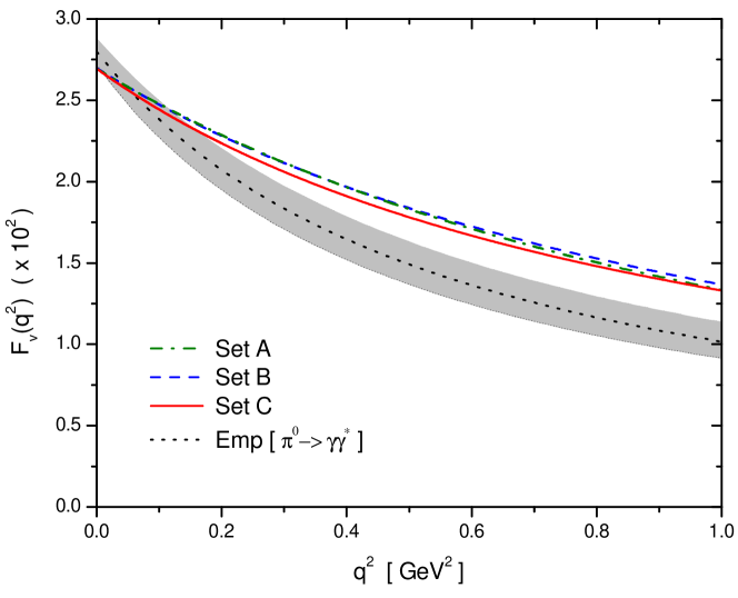
Figure 2: $F_{V}(q^{2})$ for sets $A$, $B$ and $C$. The shadowed region corresponds to empirical data on $F^{\pi\gamma\gamma^{\ast}}$, using Eqs. (21) and (22)

Our results for $F_{V}(q^{2})$ are displayed in Fig. 2, where we plot the curves corresponding to the form factors introduced in the previous section. In addition, in Fig. 2 we show the results obtained from the combination of Eq. (22) with the parameterization in Eq. (21). The parameters are taken from the experimental fit to $\pi^{0}\to\gamma\gamma^{*}$ data, which yields $F^{\pi\gamma\gamma^{\ast}}(0)=0.284(8)$ $\mbox{GeV}^{-1}$, $a_{V}^{\prime}=0.032(4)$ pdg . In general, it is seen that the results for our parameter sets A, B and C turn out to be similar in the whole range of $q^{2}$ values considered. The particular values at $q^{2}=0$ are given in Table I. As already remarked in Ref. Dumm:2010hh , one expect these values to be basically coincident given the above mentioned constraint in the chiral limit. Concerning the $q^{2}$ dependence, it is interesting to note that for all three parameter sets the behavior can be very well reproduced by a single-pole fit of the form

$$F_{V}(q^{2})=\frac{F_{V}(0)}{1+a_{V}\ q^{2}/m_{\pi}^{2}}\ .$$ (23)

In view of the relation Eq. (22), in our model $a_{V}$ can be strictly identified with the parameter $a^{\prime}_{V}$ introduced in Eq. (21).

On the other hand, it is possible to analyze the $q^{2}$ dependence of the vector form factor considering the experimental data obtained from the process $\pi^{+}\rightarrow e^{+}\nu_{e}\gamma$. For low values of $q^{2}$ one can carry out an expansion of the type

$$F_{V}(q^{2})=F_{V}(0)\,\left[1-\lambda_{V}\,\frac{q^{2}}{m_{\pi^{+}}^{2}}+\lambda_{V}^{\prime}\,\frac{q^{4}}{m_{\pi^{+}}^{4}}\right]\ ,$$ (24)

where the minus sign arises from the definition of $\lambda_{V}=m_{\pi}^{2}F_{V}^{\prime}(0)/F_{V}(0)$ for $q^{2}$ in Minkowski space. In Table I the values of $\lambda_{V},$ $\lambda_{V}^{\prime}$ and $a_{V}$ are given. We observe that $a_{V}$ is slightly different from the value of $\lambda_{V}$. The discrepancy can be taken as measure how much the actual $q^{2}$ dependence of the vector form factors deviates from the single-pole behavior. This slight deviation can be also seen from the closeness between $\lambda_{V}^{2}$ and $\lambda_{V}^{\prime}$, which should be equal in the single-pole limit. In general, it is seen that for all three parameterizations the results for $\lambda_{V}$ and $a_{V}$ are lower than experimental estimates (notice that some enhancement is found when going from sets A, B to the lattice-inspired set C). We remark that, given the fact that the calculated values of $F_{V}(q^{2})$ are well adjusted by the single-pole fit in Eq. (23), the discrepancies between the model predictions and the empirical fit observed in Fig. 2 can be traced back to the values of $a_{V}$ (or $\lambda_{V}$), i.e. the slopes of the curves at $q^{2}=0$. In fact, these discrepancies are not unexpected, since our model does not include vector-vector interactions. The magnitude of the corresponding corrections can be estimated by considering e.g. the extended NJL model studied in Ref. Prades:1993ys : indeed, it is seen that the vector contribution to $\pi^{0}\rightarrow\gamma\gamma^{\ast}$ has the right order of magnitude and sign in order to account for the discrepancies. It is also interesting to point out that the contribution from the vector channel could be different for $a_{V}$ and $a^{\prime}_{V}$, even when isospin symmetry is preserved. This would be achieved if one has different interactions in the vector-isoscalar channel and in the vector-isovector channel. As a final comment concerning the vector form factor, let us discuss the path dependence of our results. Contrary to what happens at $q^{2}=0$, the values obtained at finite $q^{2}$ depend on the path considered in Eq. (17). As usual, we have chosen a straight line path for the calculations of the path dependent quantities $\alpha_{h}^{\pm}(\ell,q)$, Eq. (20). To estimate the significance of this path dependence we have performed single-pole fits to the predictions obtained by neglecting the contribution of the the corresponding terms in Eq. (19). The resulting values for $a_{V}$ turn out to differ from the values listed in Table I by less than 0.5 %.

We turn now to the axial form factor $F_{A}(q^{2})$. Contrary to the case of the vector form factor, $F_{A}(q^{2})$ is not experimentally accessible for (Euclidean) $q^{2}>0$. As stated, the value of $F_{A}(0)$ has been measured from $\pi^{+}\rightarrow e^{+}\nu_{e}\gamma$ decay, and forthcoming experiments offer the possibility of determining the slope $F_{A}^{\prime}(0)=-F_{A}\left(0\right)\,\lambda_{A}/m_{\pi^{+}}^{2}$. The model predictions for these quantities are given in Table II. As it was discussed in Ref. Dumm:2010hh , for $F_{A}(0)$ the triangle diagram in Fig. 1a turns out to be the dominant one, giving at least 98% of the total value for all three parameter sets considered here. In the case of the slope the triangle diagram is still the dominant one, but the contributions from diagrams in Figs. 1b and 1e are also significant. One should note that nonlocal models of the type considered here lead to values of $F_{A}(0)$ which are significantly different from those of $F_{V}(0)$. This is remarkable, since other approaches like the NJL model Courtoy:2007vy or the spectral quark model Broniowski:2007fs tend to give $F_{V}(0)\simeq F_{A}(0)$. Given the triangle diagram dominance mentioned above, the origin of this difference can be traced back to the different dressing of the $\gamma_{\mu}$ and $\gamma_{\mu}\gamma_{5}$ terms in the coupling of the $W$ to the quarks Noguera:2008 . From Table II it is seen that the predictions for $F_{A}(0)$ in nonlocal models are significantly closer than the experimental value than the result obtained in the standard NJL model. Regarding the slope parameter $\lambda_{A}$, we find that our predictions are quite similar for the three parameter sets considered, and turn out to be about 3/5 smaller than the value obtained in a resonance effective model Mateu:2007tr .

IV Predictions for LECs of Chiral Perturbation Theory

In the previous section we have focused our attention on the ability of our quark models to reproduce the main features of the vector and axial-vector form factors. An alternative point of view (see for example Ref. (Schuren:1991sc, )) is to consider quark models as the generators of the pion $\chi$PT Lagrangian (Gasser:1983yg, ). $\chi$PT describes the low energy physics of pions in a universal way, once the order in the momentum and chiral breaking expansion (i.e. the order in the chiral expansion) is specified. Different scenarios for quark models will lead to $\chi$PT Lagrangians with different values of the corresponding low energy constants (LECs). In this section we analyze the connection between our quark scenarios and the $\chi$PT Lagrangian up to the fourth order in the chiral expansion.

The pionic Lagrangian that follows from performing a fourth order gradient expansion of our model bosonized action in the presence of external fields can be obtained using, for example, the method described in Ref. Schuren:1991sc . On general grounds, it should read

$$\mathcal{L}\ =\ \mathcal{L}_{2}+\mathcal{L}_{4}\ ,$$ (25)

where

$$\mathcal{L}_{2} = \frac{f^{2}}{2}\ \nabla_{\mu}U^{T}\ \nabla^{\mu}U+\ f^{2}\ \chi^{T}\ U\ \ ,$$ (26)

$$\mathcal{L}_{4} = \ell_{1}\left(\nabla_{\mu}U^{T}\ \nabla^{\mu}U\right)^{2}+\ell_{2}\left(\nabla_{\mu}U^{T}\ \nabla_{\nu}U\right)\left(\nabla^{\mu}U^{T}\ \nabla^{\nu}U\right)+\ell_{3}\left(\chi^{T}U\right)^{2}+$$ (27)

$$\ell_{4}\left(\nabla_{\mu}\chi^{T}\ \nabla^{\mu}U\right)^{2}+\ell_{5}\ U^{T}F_{\mu\nu}F^{\mu\nu}U+\ell_{6}\ \nabla^{\mu}U^{T}F_{\mu\nu}\nabla^{\nu}U+...\ \ ,$$

Here, $U=(s,p_{i})$ is a four-component real O(4) vector field of unit length, $U^{T}U=1$, and $\chi=2B(S,P_{i})$ is another O(4) vector proportional to the external scalar and pseudoescalar fields. The constant $B$ is related to the vacuum expectation value of quarks in the chiral limit and it can be expressed as $B=m^{2}/2m_{c}$ where $m$ is the pion mass at leading order in the chiral expansion. This notation follows that of Ref. (Gasser:1983yg, ) where the definition of the covariant derivative $\nabla_{\mu}$ and the field strength tensor $F_{\mu\nu}$ can be also found. Note that among all possible terms in ${\cal L}_{4}$ only those relevant for our calculation have been explicitly given.

As a result of the procedure that leads to Eq. (25) the explicit expressions for the LECs in terms of model parameters and form factors $g_{p}$ and $f_{p}$ can be obtained and eventually numerically calculated. However, a simpler and more direct way to obtain their numerical values is to extract them from the model predictions for the physical quantities they are related to. Of course, when proceeding in this way some care must be taken. In fact, since the Lagrangian in Eq. (25) is valid up to fourth order in the chiral expansion, to extract the corresponding LECs from the physical quantities obtained in our quark scenarios we should treat them to the same order of approximation. Namely, we should calculate the relevant quantities in the chiral limit and its vicinity. As described in detailed in Ref. Noguera:2008 , following this method the LECs $\ell_{1},...,\ell_{4}$ can be obtained from the predicted $\pi-\pi$ scattering parameters. Thus, in what follows we will concentrate on the remaining two parameters in Eq. (27), namely $\ell_{5}$ and $\ell_{6}$. These are related to the pion charge radius $\left\langle r^{2}\right\rangle_{\pi}$ and $F_{A}\left(0\right)/m_{\pi}$ by Gasser:1983yg

$$\ell_{5} =\frac{1}{4}\left(\frac{f_{\pi}\,F_{A}\left(0\right)}{\sqrt{2}\,m_{\pi}}-\frac{1}{3}\left\langle r^{2}\right\rangle_{\pi}\,f_{\pi}^{\,2}\right)\ ,$$

$$\ell_{6} =-\frac{1}{6}\left\langle r^{2}\right\rangle_{\pi}f_{\pi}^{\,2}\ .$$ (28)

The required chiral limit values of $f_{\pi},$ $F_{A}\left(0\right)/m_{\pi}$ and $\left\langle r^{2}\right\rangle_{\pi}$ for our three parameterizations of nonlocal quark models are given in Table III. The numerical results for $\ell_{5}$ and $\ell_{6}$ are given in Table IV, together with recent phenomenological values obtained in $\chi$PT GonzalezAlonso:2008rf and the values predicted within the Nambu-Jona Lasinio model Schuren:1991sc . For completeness we have also included the values of $\ell_{1},...,\ell_{4}$ from Ref. Noguera:2008 .

We observe that both the sign and the order of magnitude of the different LECs are in reasonably good agreement with the results from $\chi$PT for $\mu\sim 2m_{\pi}$. In fact, as already stressed in Ref. Noguera:2008 , for Set C the constants $\ell_{2}$ and $\ell_{4}$ are particularly very well reproduced, whereas the value of $\ell_{3}$ is acceptable given the existing uncertainty. For $\ell_{1}$ we obtain a rather large range of values when moving from one set of parameters to the other, but there is also a significative variation of this LEC with the choice of $\mu$. Looking at the two new LECs, $\ell_{5}$ and $\ell_{6}$, we find that the (absolute) values obtained are relatively low, and the agreement with the phenomenological values from $\chi$PT can be achieved only for somewhat larger values of the renormalization point, $\mu\gtrsim m_{\rho}$. This can be understood taking into account that our models do not include vector and axial-vector currents. Therefore, even if the quark couplings lead to some interaction in these channels, the models do not account for the effect of vector and axial-vector meson resonances. This is consistent with the analysis of Ref. CERN-TH-5185/88 , which shows that $\ell_{5}$ and $\ell_{6}$ are strongly dependent of the vector and axial-vector meson contributions. In fact, previous works on the pion electromagnetic radius including resonances indicate that vector meson contributions can give about 10$-$20% of the total result nucl-th/9910033 ; hep-ph/0311359 .

V Conclusions

We have studied the vector and axial-vector form factors in $\pi^{+}\rightarrow e^{+}\nu_{e}\gamma$ in the framework of nonlocal chiral quark models using three different sets of model parameters. As an extension of a previous work Dumm:2010hh where we have determined the values of $F_{V}(0)$, $F_{A}(0)$ and $F^{\prime}_{V}(0)$, here we have analyzed the vector form factor for values of $q^{2}$ up to 1 GeV² as well as the slope of $F_{A}(q^{2})$ at threshold. While the latter is interesting in view of the comparison with future experimental results, the study of the behavior of $F_{V}(q^{2})$ presents relevant theoretical motivations, since it can be related to the form factor $F^{\pi\gamma\gamma^{\ast}}(q^{2})$ associated with the vertex $\pi\gamma\gamma^{\ast}$. We have found that the model predictions for the $q^{2}$-dependence of the vector form factor can be well described by a single-pole parameterization. This is indicated by the fact that there is a slight difference between the values of the parameters $a_{V}$ and $\lambda_{V}$ for our three model parametrizations [the parameters $a_{V}$ and $\lambda_{V}$ are defined by Eqs. (23) and (24)]. On the other hand, it is found that for all three parametrizations our results for $a_{V}$ and $\lambda_{V}$ are below experimental estimates. These discrepancies are not unexpected, since our model does not include vector-vector interactions. In fact, a simple estimate based on an extended NJL model Prades:1993ys indicates that the vector contribution to $\pi^{0}\rightarrow\gamma\gamma^{\ast}$ has the right order of magnitude and sign in order to account for the differences. This could be tested for the present nonlocal models that include wave function renormalization through the explicit inclusion of vector-vector interactions. Regarding the slope parameter $\lambda_{A}$, we find that our predictions are quite similar for the three parameter sets considered, and turn out to be about 3/5 smaller than the value obtained in a resonance effective model Mateu:2007tr . Finally, we also have extended the analysis of Ref. Noguera:2008 , where the compatibility of our nonlocal models with effective meson theories such as $\chi$PT is studied. Indeed, we have been able to extract the model predictions for the $\chi$PT low energy constants (LECs) $\ell_{5}$ and $\ell_{6}$, taking into account the relation between these LECs and the values of $F_{A}(0)$ and the pion charge radius $\langle r^{2}\rangle_{\pi}$. Considering the results for $\ell_{5}$ and $\ell_{6}$ together with the values of $\ell_{1},..,\ell_{4}$ previously obtained in Ref. Noguera:2008 , we observe that the predictions for both the sign and the order of magnitude of the LECs within the present non-local models are in overall reasonably good agreement with the results from $\chi$PT. For the particular case of $\ell_{5}$ and $\ell_{6}$, we find that the (absolute) values obtained are somewhat small, a fact that as in the case of $a_{V}$ and $\lambda_{V}$ might be attributed to the lack of explicit vector and axial-vector interactions in our models. In any case, it is seen that nonlocal model predictions for $\ell_{5}$ are closer to the result of $\chi$PT than the value obtained in the framework of the local NJL model.

APPENDIX I: Explicit expressions for $F_{A}(q^{2})$

In this appendix we present the expressions for the contributions of the different diagrams in Fig. 1 to the axial form factor $F_{A}(q^{2})$. Let us start by the triangle diagram in Fig. 1a, which yields

$$\frac{F_{A}(q^{2})}{m_{\pi}}\Big{|}_{a} =-N_{c}\,\sqrt{2}\ G_{\pi q\bar{q}}\int\frac{d^{4}\ell}{\left(2\pi\right)^{4}}\ g_{\ell^{+}_{k-q}}\ \frac{z_{\ell+k}\ z_{\ell-q}\ z_{\ell}}{D_{\ell+k}\ D_{\ell-q}\ D_{\ell}}\left\{A_{5}\left(A\,c_{1}+B\,c_{2}+C\,c_{3}\right)\right.$$

$$\left.\qquad\qquad\qquad+B_{5}\left(A\,c_{4}+B\,c_{5}+C\,c_{6}\right)+C_{5}\left(A\,c_{7}+B\,c_{8}+C\,c_{9}\right)\right\}\ ,$$ (29)

where

$$A =\frac{1}{2}\left[\frac{1}{z_{\ell+k}}+\frac{1}{z_{\ell}}\right]\qquad;\qquad\!\!\!\!\!\!A_{5}=\frac{1}{2}\left[\frac{1}{z_{\ell}}+\frac{1}{z_{\ell-q}}\right]$$

$$B =\frac{1}{2\ell\cdot k}\left[\frac{1}{z_{\ell}}-\frac{1}{z_{\ell+k}}\right]\ \ ;\qquad\!\!\!\!\!\!\!\!B_{5}=\frac{1}{2\ q\cdot\ell_{q}^{-}}\left[\frac{1}{z_{\ell-q}}-\frac{1}{z_{\ell}}\right]+\frac{q^{2}\,\bar{\sigma}_{2}}{2\ q\cdot\ell_{q}^{-}}\alpha^{+}_{f}\left(\ell^{-}_{q},q\right)$$

$$C =\frac{1}{\ell\cdot k}\left[\frac{m_{\ell+k}}{z_{\ell+k}}-\frac{m_{\ell}}{z_{\ell}}\right]\ \ ;\qquad\!\!\!\!\!\!\!\!\!C_{5}=\frac{1}{q\cdot\ell_{q}^{-}}\left[2\frac{m_{\ell^{-}_{q}}}{z_{\ell^{-}_{q}}}-\frac{m_{\ell}}{z_{\ell}}-\frac{m_{\ell-q}}{z_{\ell-q}}\right]+\frac{q^{2}\,\bar{\sigma}_{1}}{q\cdot\ell_{q}^{-}}\alpha^{-}_{g}\left(\ell^{-}_{q},q\right)\ .$$ (30)

Here, and in what follows, we use the already introduced shorthand notation $\ell^{\pm}_{r}=\ell\pm r/2$, together with the functions $\alpha^{\pm}_{h}(\ell,q)$ defined in Eq. (20). The coefficients $c_{i}$ with $i=1,...,9$ are given by

$$c_{1} =2\,e_{1}\,\left(m_{\ell+k}-m_{\ell-q}\right)+2\,e_{2}\,\left(m_{\ell}-m_{\ell+k}\right)-2\,e_{3}\,\left(m_{\ell}+m_{\ell-q}\right)+4m_{\ell}$$

$$c_{2} =e_{1}\left[-2k\cdot\ell\left(2m_{\ell}+m_{\ell+k}-m_{\ell-q}\right)-2d_{1}+k\cdot q\left(m_{\ell}+m_{\ell+k}\right)\right]$$

$$\qquad\qquad\qquad\qquad+2\,e_{3}\left[d_{3}-\ell\cdot q\left(m_{\ell}+m_{\ell+k}\right)\right]$$

$$c_{3} =e_{1}\,\left[k\cdot q-2\ k\cdot\ell+d_{4}-d_{6}\right]-2\,e_{3}\left[d_{5}-2\ell^{2}+\ell\cdot q\right]$$

$$c_{4} =e_{1}\left[-2d_{1}+2\ell\cdot q\left(m_{\ell+k}+2m_{\ell}-m_{\ell-q}\right)-q^{2}\left(m_{\ell}+m_{\ell+k}\right)+k\cdot q\left(m_{\ell}-m_{\ell-q}\right)\right]$$

$$\qquad+2\,e_{2}\left[k\cdot\ell\left(m_{\ell-q}-m_{\ell}\right)+d_{2}\right]$$

$$c_{5} =e_{1}\,\left[\left(4k\cdot\ell+4\ \ell^{2}-4\ell\cdot q-k\cdot q\right)\,d_{1}-2\,k\cdot\ell\,d_{2}-2\,\ell\cdot q\,d_{3}\right.$$

$$\left.-2\,k\cdot\ell\,\ell\cdot q\left(4m_{\ell}+m_{\ell+k}-m_{\ell-q}\right)+q^{2}\,\left(2\,\ell^{2}\left(m_{\ell}+m_{\ell+k}\right)+k\cdot\ell\left(3m_{\ell}+m_{\ell+k}\right)\right)\right]$$

$$c_{6} =e_{1}\,\left[k\cdot\ell\left[2\,d_{5}-2\ell\cdot q+q^{2}\right]+\left(2\ell^{2}-\ell\cdot q\right)\,d_{6}-d_{4}\,\left(2\ell^{2}-3\ell\cdot q+q^{2}\right)-k\cdot q\,d_{5}\right]$$

$$c_{7} =e_{1}\,\left[d_{6}-d_{4}-2\,\ell\cdot q-k\cdot q\right]+2\,e_{2}\,\left[d_{4}+2\ell^{2}+k\cdot\ell\right]$$

$$c_{8} =e_{1}\,\left[2\,k\cdot\ell\left(\ell\cdot q-d_{5}\right)-\left(2\,\ell^{2}+k\cdot\ell\right)\,d_{6}+\left(2\,\ell^{2}-2\,\ell\cdot q-k\cdot q+k\cdot\ell\right)\,d_{4}\right]$$

$$c_{9} =e_{1}\,\left[d_{1}-k\cdot\ell\left(m_{\ell-q}-m_{\ell}\right)-\ell\cdot q\left(m_{\ell}+m_{\ell+k}\right)-k\cdot q\ m_{\ell}\right]\ ,$$ (31)

where

$$\begin{array}[c]{lcl}d_{1}=\ell^{2}\left(m_{\ell}+m_{\ell+k}-m_{\ell-q}\right)+m_{\ell-q}\,m_{\ell}\,m_{\ell+k}&&d_{4}=m_{\ell}\,m_{\ell+k}-\ell^{2}\\ d_{2}=\ell^{2}\left(m_{\ell-q}+m_{\ell+k}-m_{\ell}\right)+m_{\ell-q}\,m_{\ell}\,m_{\ell+k}&&d_{5}=m_{\ell}\,m_{\ell-q}+\ell^{2}\\ d_{3}=\ell^{2}\left(m_{\ell}+m_{\ell+k}+m_{\ell-q}\right)-m_{\ell-q}\,m_{\ell}\,m_{\ell+k}&&d_{6}=m_{\ell-q}\,\left(m_{\ell}+m_{\ell+k}\right)\end{array}$$ (32)

and

$$e_{1}=-\frac{6\;q^{2}\;(k\cdot\ell)^{2}}{(k\cdot q)^{3}}+\frac{8\;k\cdot\ell\ \ell\cdot q}{(k\cdot q)^{2}}-\frac{2\;\ell^{2}}{k\cdot q}\ ;\ e_{2}=-\frac{2\;q^{2}\;k\cdot\ell}{(k\cdot q)^{2}}+2\ \frac{\ell\cdot q}{k\cdot q}\ ;\ e_{3}=\frac{2\;k\cdot\ell}{k\cdot q}\ .$$ (33)

The contributions of the other diagrams are the following:

$$\frac{F_{A}(q^{2})}{m_{\pi}^{+}}\Big{|}_{b} = -\frac{\sqrt{2}}{2}\,G_{\pi q\bar{q}}\,N_{c}\int\frac{d^{4}\ell}{\left(2\pi\right)^{4}}\,\frac{e_{1}}{\ell\cdot k}\,\left(2\,g_{\ell}-g_{\ell^{-}_{k}}-g_{\ell^{+}_{k}}\right)\frac{z_{\ell^{+}_{q}}}{D_{\ell^{+}_{q}}}\,\frac{z_{\ell^{-}_{q}}}{D_{\ell^{-}_{q}}}\Bigg{\{}\frac{m_{\ell^{+}_{q}}}{z_{\ell^{-}_{q}}}-\frac{m_{\ell^{-}_{q}}}{z_{\ell^{+}_{q}}}$$

$$+\left(\frac{1}{z_{\ell^{+}_{q}}}-\frac{1}{z_{\ell^{-}_{q}}}\right)\frac{m_{\ell^{+}_{q}}-m_{\ell^{-}_{q}}}{\ell\cdot q}\,\ell^{2}+\left(2\,\frac{m_{\ell}}{z_{\ell}}-\frac{m_{\ell^{+}_{q}}}{z_{\ell^{+}_{q}}}-\frac{m_{\ell^{-}_{q}}}{z_{\ell^{-}_{q}}}\right)\,\frac{\ell^{+}_{q}\cdot\ell^{-}_{q}+m_{\ell^{+}_{q}}\,m_{\ell^{-}_{q}}}{\ell\cdot q}$$

$$-\,\frac{q^{2}}{\ell\cdot q}\Bigg{[}\bar{\sigma}_{1}\,\alpha^{-}_{g}\left(\ell,q\right)\left[\ell^{+}_{q}\cdot\ell^{-}_{q}+m_{\ell^{+}_{q}}\,m_{\ell^{-}_{q}}\right]\!+\,\bar{\sigma}_{2}\,\alpha^{+}_{f}\left(\ell,q\right)\,\ell\cdot\left[\ell^{-}_{q}\,m_{\ell^{+}_{q}}-\ell^{+}_{q}\,m_{\ell^{-}_{q}}\right]\!\Bigg{]}\Bigg{\}}$$

$$\frac{F_{A}(q^{2})}{m_{\pi}^{+}}\Big{|}_{c} = \sqrt{2}\ G_{\pi q\bar{q}}\ N_{c}\int\frac{d^{4}\ell}{(2\pi)^{4}}\ \frac{e_{1}}{\ell\cdot k\ \ell\cdot q}\left[\frac{z_{\ell_{k}^{-}}m_{\ell_{k}^{-}}}{D_{\ell_{k}^{-}}}-\frac{z_{\ell_{k}^{+}}m_{\ell_{k}^{+}}}{D_{\ell_{k}^{+}}}\right]\left[g_{\ell_{q}^{+}}+\frac{q^{2}}{2}\ \alpha^{+}_{g}(\ell,q)\right]$$

$$\frac{F_{A}(q)}{m_{\pi^{+}}}\Big{|}_{d} = \sqrt{2}\ G_{\pi q\bar{q}}\ N_{c}\int\frac{d^{4}\ell}{(2\pi)^{4}}\ \ \frac{e_{1}}{k\cdot\ell\ q\cdot\ell}\left[\frac{z_{\ell^{-}_{k}}\ m_{\ell^{-}_{k}}}{D_{\ell^{-}_{k}}}-\frac{z_{\ell}\ m_{\ell}}{D_{\ell}}\right]$$

$$\qquad\qquad\qquad\qquad\times\left[g_{\ell^{+}_{q}}-g_{\ell}-\frac{q^{2}}{2}\,\left(\alpha^{+}_{g}(\ell,q)+\alpha^{-}_{g}(\ell,q)\right)\right]$$

$$\frac{F_{A}(q^{2})}{m_{\pi}}\Big{|}_{e} = -\sqrt{2}\,G_{\pi q\bar{q}}\,N_{c}\int\frac{d^{4}\ell}{\left(2\pi\right)^{4}}\,g_{\ell}\frac{z_{\ell^{+}_{k+q}}}{D_{\ell^{+}_{k+q}}}\,\frac{z_{\ell^{-}_{k+q}}}{D_{\ell^{-}_{k+q}}}\Bigg{\{}\bar{\sigma}_{1}\left[\ell^{+}_{k+q}\cdot\ell^{-}_{k+q}+m_{\ell^{+}_{k+q}}\,m_{\ell^{-}_{k+q}}\right]\frac{\mathcal{\eta}_{g}\left(\ell,k,q\right)}{\left(k\cdot q\right)^{2}}$$ (34)

$$-\bar{\sigma}_{2}\left[m_{\ell^{-}_{k+q}}\ \ell\cdot\ell^{+}_{k+q}-m_{\ell^{+}_{k+q}}\ \ell\cdot\ell^{-}_{k+q}\right]\frac{\mathcal{\eta}_{f}\left(\ell,k,q\right)}{\left(k\cdot q\right)^{2}}$$

$$+\frac{1}{2\;k\cdot\ell^{+}_{q}}\,\left[\frac{1}{z_{\ell^{+}_{q-k}}}-\frac{1}{z_{\ell^{+}_{k+q}}}\right]\left[m_{\ell^{+}_{k+q}}\left(e_{1}+e_{2}-e_{3}-1\right)-m_{\ell^{-}_{k+q}}\left(e_{1}+e_{2}+e_{3}+1\right)\right]$$

$$+\frac{1}{2\;q\cdot\ell^{-}_{k}}\,\left[\frac{1}{z_{\ell^{-}_{k+q}}}-\frac{1}{z_{\ell^{+}_{q-k}}}+q^{2}\,\bar{\sigma}_{2}\,\alpha^{+}_{f}\left(\ell^{-}_{k},q\right)\right]\left[m_{\ell^{+}_{k+q}}\left(e_{1}-e_{2}-e_{3}+1\right)\right.$$

$$\left.\qquad\qquad\qquad\qquad\qquad\qquad\qquad\qquad\qquad\ -\ m_{\ell^{-}_{k+q}}\left(e_{1}+e_{2}-e_{3}-1\right)\right]\Bigg{\}}$$

where

$$\eta_{h}(\ell,k,q) =(k.q)^{2}\int_{0}^{1}d\lambda\int_{-1}^{0}d\lambda^{\prime}\ \left(e_{1}+e_{2}\lambda+e_{3}\lambda^{\prime}+\lambda\lambda^{\prime}\right)h^{\prime\prime}_{\ell^{+}_{\lambda q+\lambda^{\prime}k}}$$ (35)

for $h=g$ or $f$.

Table 1: Results for $F_{V}(q^{2})$ and its first and second derivative at $q^{2}=0$. All results should be multiplied by $10^{-2}$. In column 5 we give the empirical values of $m_{\pi^{+}}\,F^{\pi\gamma\gamma^{\ast}}(0)/\sqrt{2}$ and $a^{\prime}_{V}$. Note that in our model $a_{V}=a_{V}^{\prime}$. In column 6 we give the prediction of the local Nambu–Jona-Lasinio (NJL) model.

	Set A	Set B	Set C	Exp Bychkov:2008ws	Exp ($\pi^{0}\rightarrow\gamma\gamma^{\ast})$pdg	NJL	Ref Mateu:2007tr
$F_{V}(0)$	2.697	2.693	2.695	2.58(17)	2.80(8)	2.441	2.71
$a_{V}$	1.91	1.87	1.98		3.2(4)
$\lambda_{V}$	1.651	1.726	2.011	10(6)		3.244	4.1
$\lambda_{V}^{\prime}$	0.020	0.026	0.046			$-$

Table 2: Results for $F_{A}(q^{2})$ and its first and second derivative at $q^{2}=0$. All results should be multiplied by $10^{-2}$. In column 5 we give the prediction of the local Nambu–Jona-Lasinio (NJL) model.

	Set A	Set B	Set C	Exp Bychkov:2008ws	NJL	From Mateu:2007tr
$F_{A}(0)$	1.319	1.614	1.825	1.17 $\pm$ 0.17	2.409	exp. input
$\lambda_{A}$	1.22	1.17	1.26		$-$	1.97
$\lambda_{A}^{\prime}$	0.012	0.013	0.034		$-$

Table 3: Physical quantities used in the evaluation of $\ell_{5,6}$ obtained in our different scenarios in the chiral limit.

		SA	SB	SC
$\left\langle r^{2}\right\rangle_{\pi}$	fm2	0.335	0.325	0.316
$F_{A}(0)/m_{\pi}$	GeV-1	0.097	0.118	0.133
$f_{\pi}$	MeV	91.2	91.4	91.8

Table 4: Values of $\ell_{i}$ obtained in our different scenarios. The $\chi$PT values of $\ell_{i}^{r}$ as a function of $\mu$ are obtained from Refs. Colangelo:2001df ; GonzalezAlonso:2008rf . The last two columns corresponds to the NJL predictions from Ref. Schuren:1991sc for two different constituent quark mass: $M=220,264\,\mathrm{MeV}$

.

LEC	Non Local QM				$\chi$PT ($\ell_{i}^{r}(\mu)$)				NJL
$\times 10^{3}$	SA	SB	SC		$\mu=m_{\rho}$	$\ \ \ \mu=2\ m_{\pi}$	$\ \ \mu=m_{\pi}$		$M=220$	$M=264$
$\ell_{1}$	-2.07	-1.39	0.26		$-4.0\pm 0.6$	$-1.9\pm 0.6$	$-0.4\pm 0.6$		-0.63	-2.3
$\ell_{2}$	6.51	6.46	6.41		$1.9\pm 0.2$	$6.2\pm 0.2$	$9.1\pm 0.2$		6.3	6.2
$\ell_{3}$	-1.1	-2.3	-4.1		$1.5\pm 4.0$	$-1.8\pm 4.0$	$-4.0\pm 4.0$		-8.5	-3.5
$\ell_{4}$	15.0	17.2	20.3		$6.2\pm 1.3$	$19.1\pm 1.3$	$27.9\pm 1.3$		22.7	12.2
$\ell_{5}$	-4.39	-3.90	-3.54		$~{}-5.22\pm 0.06$	$~{}-6.29\pm 0.06$	$~{}-7.02\pm 0.06$		-2.88	-2.60
$\ell_{6}$	-11.9	-11.6	-11.4		$-13.1\pm 0.4$	$-15.3\pm 0.4$	$-16.8\pm 0.4$		-11.5	-10.4
$\left(2\,\ell_{5}-\ell_{6}\right)$	3.15	3.82	4.33		$2.7\pm 0.4$	$2.7\pm 0.4$	$2.7\pm 0.4$		5.75	5.21

Figure 1: Diagrammatic representation of the possible contributions to $\pi^{+}\rightarrow e^{+}\nu_{e}\gamma$ decay. Double-dashed lines, wavy lines and single-dashed lines represent the $e\,\nu_{e}$ pair, the outgoing photon and the decaying pion, respectively. While for the vector form factor only the contribution from the triangle diagram (a) is nonvanishing, in the case of the axial-vector form factor all five diagrams contribute.

.

References

- (1) M. Moreno, Phys. Rev. D 16 (1977) 720; D. A. Bryman, P. Depommier and C. Leroy, Phys. Rept. 88 (1982) 151.
- (2) M. Bychkov et al., Phys. Rev. Lett. 103 (2009) 051802 [arXiv:0804.1815 [hep-ex]].
- (3) B. R. Holstein, Phys. Rev. D 33 (1986) 3316; J. Bijnens and P. Talavera, Nucl. Phys. B 489 (1997) 387 [arXiv:hep-ph/9610269]; C. Q. Geng, I. L. Ho and T. H. Wu, Nucl. Phys. B 684 (2004) 281 [arXiv:hep-ph/0306165].
- (4) V. Mateu and J. Portoles, Eur. Phys. J. C 52 (2007) 325 [arXiv:0706.1039 [hep-ph]].
- (5) U. Vogl and W. Weise, Prog. Part. Nucl. Phys. 27 (1991) 195.
- (6) S. P. Klevansky, Rev. Mod. Phys. 64 (1992) 649.
- (7) T. Hatsuda and T. Kunihiro, Phys. Rept. 247 (1994) 221.
- (8) G. Ripka, Quarks bound by chiral fields (Oxford University Press, Oxford, 1997).
- (9) T. Schafer and E. V. Shuryak, Rev. Mod. Phys. 70 (1998) 323 [arXiv:hep-ph/9610451].
- (10) C. D. Roberts and A. G. Williams, Prog. Part. Nucl. Phys. 33 (1994) 477 [arXiv:hep-ph/9403224]; C. D. Roberts and S. M. Schmidt, Prog. Part. Nucl. Phys. 45 (2000) S1 [arXiv:nucl-th/0005064].
- (11) M. B. Parappilly, P. O. Bowman, U. M. Heller, D. B. Leinweber, A. G. Williams and J. B. Zhang, Phys. Rev. D 73 (2006) 054504 [arXiv:hep-lat/0511007].
- (12) P. O. Bowman, U. M. Heller, D. B. Leinweber and A. G. Williams, Nucl. Phys. Proc. Suppl. 119 (2003) 323. [arXiv:hep-lat/0209129]. P. O. Bowman, U. M. Heller, and A. G. Williams, Phys. Rev. D 66 (2002) 014505. [arXiv:hep-lat/0203001].
- (13) S. Furui and H. Nakajima, Phys. Rev. D 73 (2006) 074503.
- (14) R. D. Bowler and M. C. Birse, Nucl. Phys. A 582 (1995) 655 [arXiv:hep-ph/9407336]; R. S. Plant and M. C. Birse, Nucl. Phys. A 628 (1998) 607 [arXiv:hep-ph/9705372].
- (15) A. Scarpettini, D. Gomez Dumm and N. N. Scoccola, Phys. Rev. D 69 (2004) 114018 [arXiv:hep-ph/0311030].
- (16) D. Gomez Dumm, A. G. Grunfeld and N. N. Scoccola, Phys. Rev. D 74 (2006) 054026 [arXiv:hep-ph/0607023].
- (17) B. Golli, W. Broniowski and G. Ripka, Phys. Lett. B 437 (1998) 24 [arXiv:hep-ph/9807261]; W. Broniowski, B. Golli and G. Ripka, Nucl. Phys. A 703 (2002) 667 [arXiv:hep-ph/0107139].
- (18) A. H. Rezaeian, N. R. Walet and M. C. Birse, Phys. Rev. C 70 (2004) 065203 [arXiv:hep-ph/0408233]; A. H. Rezaeian and H. J. Pirner, Nucl. Phys. A 769 (2006) 35 [arXiv:nucl-th/0510041].
- (19) M. Praszalowicz and A. Rostworowski, Phys. Rev. D 64 (2001) 074003; Phys. Rev. D 66 (2002) 054002 [arXiv:hep-ph/0111196].
- (20) S. Noguera and V. Vento, Eur. Phys. J. A 28 (2006) 227 [arXiv:hep-ph/0505102].
- (21) S. Noguera, Int. J. Mod. Phys. E 16 (2007) 97 [arXiv:hep-ph/0806.0818]
- (22) S. Noguera and N. N. Scoccola, Phys. Rev. D 78 (2008) 114002 [arXiv:hep-ph/0806.0818].
- (23) D. Gomez Dumm, S. Noguera and N.N. Scoccola, Phys. Lett. B 698 (2011) 236.
- (24) K. Nakamura et al. (Particle Data Group), J. Phys. G 37 (2010) 075021.
- (25) J. Prades, Z. Phys. C 63 (1994) 491 [Erratum-ibid. C 11 (1999) 571] [arXiv:hep-ph/9302246].
- (26) A. Courtoy and S. Noguera, Phys. Rev. D 76 (2007) 094026 [arXiv:0707.3366 [hep-ph]].
- (27) W. Broniowski and E. R. Arriola, Phys. Lett. B 649 (2007) 49 [arXiv:hep-ph/0701243].
- (28) C. Schuren, E. Ruiz Arriola and K. Goeke, Nucl. Phys. A 547 (1992) 612.
- (29) J. Gasser and H. Leutwyler, Annals Phys. 158 (1984) 142.
- (30) G. Colangelo, J. Gasser and H. Leutwyler, Nucl. Phys. B 603, 125 (2001) [hep-ph/0103088].
- (31) M. Gonzalez-Alonso, A. Pich and J. Prades, Phys. Rev. D 78 (2008) 116012 [arXiv:0810.0760 [hep-ph]].
- (32) G. Ecker, J. Gasser, A. Pich and E. de Rafael, Nucl. Phys. B 321 (1989) 311.
- (33) P. Maris and P. C. Tandy, Phys. Rev. C 61 (2000) 045202 [nucl-th/9910033].
- (34) A. E. Dorokhov, A. E. Radzhabov and M. K. Volkov, Eur. Phys. J. A 21 (2004) 155 [hep-ph/0311359].