Spectral integration of linear boundary value problems

Abstract

Spectral integration was deployed by Orszag and co-workers (1977, 1980, 1981) to obtain stable and efficient solvers for the incompressible Navier-Stokes equation in rectangular geometries. Two methods in current use for channel flow and plane Couette flow, namely, Kleiser-Schumann (1980) and Kim-Moin-Moser (1977), rely on the same technique. In its current form, the technique of spectral integration, as applied to the Navier-Stokes equations, is dominated by rounding errors at higher Reynolds numbers which would otherwise be within reach. In this article, we derive a number of versions of spectral integration and explicate their properties, with a view to extending the Kleiser-Schumann and Kim-Moin-Moser algorithms to higher Reynolds numbers. More specifically, we show how spectral integration matrices that are banded, but bordered by dense rows, can be reduced to purely banded matrices. Key properties, such as the accuracy of spectral integration even when Green’s functions are not resolved by the underlying grid, the accuracy of spectral integration in spite of ill-conditioning of underlying linear systems, and the accuracy of derivatives, are thoroughly explained.

Department of Mathematics, University of Michigan (divakar@umich.edu).

1 Introduction

One of the earliest methods for solving the incompressible Navier-Stokes equation was proposed in a pioneering paper by Orszag [16]. In that paper, Orszag tackled the problem of numerically integrating wall-bounded shear flows using Chebyshev series expansions. The Chebyshev polynomial is defined by $T_{n}(y)=\cos\left(n\arccos y\right)$ for $-1\leq y\leq 1$. If $u(y)=\alpha_{0}T_{0}/2+\sum_{j=1}^{\infty}\alpha_{n}T_{n}$ is the Chebyshev series of $u(y)$, we denote the Chebyshev coefficient $\alpha_{n}$ by $\mathcal{T}_{n}(u)$. The points $y_{j}=\cos(j\pi/M)$, $j=0,\ldots,M$, are the Chebyshev grid points. The discrete cosine transform may be used to pass back and forth between the physical domain function values $u(y_{j})$, $0\leq j\leq M$, and the coefficients in the truncated Chebyshev expansion $\alpha_{0}T_{0}/2+\sum_{j=1}^{M-1}\alpha_{j}T_{j}+\alpha_{M}T_{M}/2$.

The method proposed by Orszag in [16] is certainly complete. However, it is much too expensive. It does not appear to have been implemented and therefore its effectiveness cannot be gaged. Nevertheless, when numerical computations of fully turbulent solutions of shear flows at last became possible nearly two decades later [12], they relied on Chebyshev series expansion in the wall-normal directions and other ideas introduced by Orszag. The two now classical methods for computing turbulent solutions of the Navier-Stokes equation are due to Kleiser-Schumann [13] and Kim-Moin-Moser [12].

The method of spectral integration was introduced by Gottlieb and Orszag as a reformulation of the tau-equations [6, p. 119]. It is the thread which links the early work of Orszag [16] with the Kleiser-Schumann and Kim-Moin-Moser methods. Below and throughout this paper, $D$ denotes $d/dy$. The Chebyshev tau equations for a boundary value problem such as

$$\left(D^{2}-a^{2}\right)u=f(y),\,u(\pm 1)=0,$$ (1.1)

are obtained by expanding the sought for solution $u$ in a truncated Chebyshev series and equating the Chebyshev coefficients of $T_{0},\ldots,T_{M-2}$ in the expansion of $\left(D^{2}-a^{2}\right)u$ to those of $f$, and enforcing the boundary conditions to get two more equations. As Gottlieb and Orszag noted the tau equations are dense and not well-conditioned. Their method of rewriting gives a tridiagonal system bordered by dense rows corresponding to the boundary conditions. In Section 2, we derive a variety of spectral integration methods. The Gottlieb-Orszag method is a special case of one of them. All the methods of Section 2 work with purely banded matrices and no bordering rows. Working with purely banded matrices enforces a key property of spectral integration explicitly, instead of relying on accident or the vagaries of implementation. This key property, explained in Section 3.1, is the cancellation of large discretization errors that arise in the intermediate stages of spectral integration. Without this property, spectral integration would be ineffective for the computation of turbulent solutions. The more accurate versions of Kleiser-Schumann and Kim-Moin-Moser derived in [20] rely upon working with purely tridiagonal systems.

The method of spectral integration was employed widely in the solution of channel flow and plane Couette flow, especially in the transitional and turbulent regimes, beginning with Orszag and coworkers [17, 18], Kleiser-Schumann [13], and Kim-Moin-Moser [12]. However, two of its key properties came to light only with the work of Greengard [7]. The Green’s function of the boundary value problem (1.1) has a scale which is $\mathcal{O}(1/a)$ and which arises from terms such as $\exp(-a|y-\tilde{y}|)$. However, the solution may not have such a fine scale. For example, we may choose $a=10^{6}$ and then $f(y)$ in such a way that $u(y)=\sin\pi y$ is the solution of the boundary value problem (1.1). In that situation one would need $M>2\times 10^{4}$ to resolve the Green’s function at the boundaries while $M=32$ suffices to resolve the solution $u(y)$. Greengard noted accurate solutions may be computed when the Chebyshev grid resolves the solution even if it fails to resolve the Green’s function.

This property appears essential for the robustness, if not the success, of spectral integration in turbulence computations. The analogue of $a$ in (1.1) in a channel flow or plane Couette flow computation is given by $a=\beta=\left(\gamma Re/\Delta t+\beta^{\ast}\right)^{1/2}$, where $\beta^{\ast}$ is positive and much smaller than $Re/\Delta t$. The Reynolds number is denoted by $Re$ and the time step by $\Delta t$; $\gamma$ is an $\mathcal{O}\left(1\right)$ parameter. The channel flow simulation in [20] has $\beta\approx 2\times 10^{4}$ and reaches $Re=80,000$. Reaching an $Re$ that is $5$ times as high will imply $\beta>10^{5}$ in the boundary value problems that arise while time stepping channel flow. The solutions themselves may not have scales as small as $\mathcal{O}\left(1/\beta\right)$, because the smallness of $1/\beta$ is partly a reflection of time stepping and not entirely due to the physics of the problem. Thus it is fortunate that spectral integration can compute accurate solutions without resolving the $1/\beta$ scale. A complete explanation of why spectral integration has this property is given in Section 3.1. The explanation relies on formulations in Section 2 which avoid bordering banded systems with dense rows.

Another property brought to light by Greengard [7] is that condition numbers of spectral integration matrices, corresponding to boundary value problems such as (1.1), are bounded in the limit $M\rightarrow\infty$. As noted by Rokhlin [19], any integral formulation has this property because the integral operators that are discretized are compact. In contrast, the tau equations discretize (1.1) in its differential form and therefore suffer from ill-conditioning. In particular, their condition number goes to $\infty$ as $M\rightarrow\infty$.

Although this is a useful property, it is by itself inadequate to understand the robustness of spectral integration as applied to the Navier-Stokes equations in the turbulent regime. If $a=10^{6}$ in the boundary value problem (1.1), for example, the condition number of the spectral integration matrices is of the order $\mathcal{O}\left(10^{12}\right)$. For $4$-th order problems such as $\left(D^{2}-a^{2}\right)\left(D^{2}-b^{2}\right)u=f$, the condition number appear to get as large as $\mathcal{O}\left(a^{2}b^{2}\right)$ in the limit $M\rightarrow\infty$. The fact that the condition numbers do not diverge as $M\rightarrow\infty$ offers little comfort when condition numbers become so large. Such large condition numbers suggest a severe loss of accuracy. Yet even in the presence of such ill-conditioning, spectral integration is able to compute solutions $u(y)$ with close to machine precision. In Section 3.2, we explain how spectral integration comes to have such remarkable accuracy.

Greengard’s form of spectral integration as applied to (1.1) expands $D^{2}u$ instead of $u$ in a Chebyshev series. Thus it may be suspected that Greengard’s form produces more accurate derivatives. In fact, that is partially but not entirely true. Building upon a discovery of Muite [14], we discuss why all forms of spectral integration produce derivatives with similar accuracy when the parameter $a$ of (1.1) is not too large. The key point, as noted by Muite, is that one must not pass into physical space when calculating derivatives. However, when $a$ is large, as in turbulence simulations with high Reynolds number, there is a significant advantage to avoiding numerical differentiation altogether.

The more robust versions of Kleiser-Schumann and Kim-Moin-Moser derived in [20] are specially adapted to either method and combine several of the forms of spectral integration derived in Section 2. They altogether avoid numerical differentiation in the wall-normal direction. The ease with which the different forms can be combined follows from the way we enforce boundary conditions. Instead of using ad-hoc bordered rows for boundary conditions, we derive the boundary conditions from integral conditions that are intrinsic to spectral integration formulations. Both the method of Gottlieb and Orszag [6, p. 119] and that of Greengard [7] are seen to be special cases.

Certain comments made by Orszag and coworkers [17, 18] show awareness of the connection of the method of Gottlieb and Orszag [6, p. 119] to integral formulations. A more explicit connection was made by Muite [14] and by Charalambides and Waleffe [3, 2]. The latter authors study spurious eigenvalues of spectral discretization matrices using the theory of stable polynomials. They consider Jacobi and Gegenbauer polynomials in addition to Chebyshev. A connection of the method of Gottlieb and Orszag to spectral integration is made at a more fundamental level in Section 2.

A number of numerical examples are included in Section 4. These examples are illustrative but do not indicate the potential of the methods derived here. When problem sizes are small, it is difficult to argue for the value of carefully derived and highly accurate methods. Therefore Section 4 discusses the Kleiser-Schumann algorithm in the context of properties of spectral integration derived in Section 2. The main application is to the integration of the Navier-Stokes equation in rectangular geometry and in the turbulent regime. In a companion paper [20], we present a computation of turbulent channel flow that reaches $Re_{\tau}=2380$ using $10^{9}$ grid points and $M=1024$. Only $10$ nodes of a small cluster are used in this computation. The computation uses an algorithm, derived using the techniques of the present paper, which avoids numerical differentiation in the wall-normal direction entirely. This computation may be compared with those of Hoyas and Jiménez [10, 11] who reached $Re_{\tau}=2003$. As explained in [20], current methods have fundamental limitations that limit them to $M\approx 1000$. The methods derived in [20] using techniques of the present paper appear capable of handling problems with $M=10^{4}$, which would take us into problem sizes beyond the reach of modern computers. Turbulence computations such as the ones in [10, 11, 20] are typically run for several months.

Beyond the application to channel flow and plane Couette flow, the methods derived here are likely to be of use in other problems in fluid mechanics such as Rayleigh-Bénard convection and Kolmogorov flow.

2 Varieties of spectral integration

In this section, the interval of the boundary value problem is taken to be $-1\leq y\leq 1$ and the solution $u$ or one of its derivatives is expanded as follows:

$$\frac{\alpha_{0}}{2}+\alpha_{1}T_{1}+\cdots+\alpha_{M-1}T_{M-1}+0.T_{M}.$$ (2.1)

The Chebyshev points $y_{j}=\cos(j\pi/M)$ with $j=0\ldots M$ are $M+1$ in number including the endpoints $\pm 1$, but the last coefficient in the Chebyshev series is suppressed for convenience as indicated in (2.1).

In each of the methods of this section including the factored form of spectral integration, the way the homogeneous solutions are computed may appear roundabout. As explained in Section 3.1, such a roundabout calculation is essential for ensuring accuracy.

The method of Gottlieb and Orszag [6, p. 119] is a special case of the method in Section 2.1. The method of Greengard [7] is a special case of the method in Section 2.3. Apart from being more general, our formulation works with purely banded systems instead of banded systems with rows. If the boundary conditions are not suitably scaled, Gaussian elimination with partial pivoting can turn a banded system with a few dense rows into a dense matrix. The use of QR factorization to solve such systems has been proposed [15]. QR with its use of square roots would be much too slow for applications such as computations of turbulence in channel flow. All these issues are swept aside by the methods given here, all of which use only purely banded systems. Another advantage is that our formulations lead to an explanation of why spectral integration schemes are accurate if they resolve the solution but not the Green’s function. This explanation is given in Section 3.1.

2.1 First and second order spectral integration

Suppose a first order boundary value problem is given in the form

$$(D-a)u=f.$$ (2.2)

The exact boundary condition is unimportant for much of the method. To begin with we assume the integral condition $\mathcal{T}_{0}(u)=0$ or equivalently $\alpha_{0}=0$. Suppose that the Chebyshev coefficients of $f$ are given by $f_{j}=\mathcal{T}_{j}(f)$.

The indefinite integral of (2.2) gives

$$u-a\int u+A=\int f,$$ (2.3)

where $A$ is an undetermined constant. The integral $\int T_{n}\,dy$ is $T_{n+1}/2(n+1)-T_{n-1}/2(n-1)$ if $n>1$, $T_{2}/4$ if $n=1$, and $T_{1}$ if $n=0$. Therefore, the coefficient of $T_{n}$ on the right hand side of (2.3) is

$$\mathcal{T}_{n}\left(\int f\right)=\frac{f_{n-1}-f_{n+1}}{2n}\quad\text{for}\quad n=1,2,\ldots,M-1.$$

The $n=M-1$ case assumes $f_{M}=0$. Similarly, the coefficient of $T_{n}$ in the expansion of the left hand side of (2.3) is

$$\mathcal{T}_{n}\left(u-a\int u+A\right)=\begin{cases}\alpha_{n}-a\left(\frac{\alpha_{n-1}-\alpha_{n+1}}{2n}\right)&2\leq n\leq M-2\\ \alpha_{n}-a\left(\frac{-\alpha_{n+1}}{2n}\right)&n=1\\ \alpha_{n}-a\left(\frac{\alpha_{n-1}}{2n}\right)&n=M-1\end{cases}$$

for $n=1,\ldots,M-1$. The coefficients with $n=1$ and $n=M-1$ are obtained from the more general expression $\alpha_{n}-a(\alpha_{n-1}-\alpha_{n+1})/2n$ by setting $\alpha_{0}=0$ and $\alpha_{M}=0$, respectively. Equating coefficients for $n=1,\ldots,M-1$ we have $M-1$ equations for the $M-1$ unknowns $\alpha_{1},\ldots,\alpha_{M-1}$. If we did not set $\alpha_{M}=0$, another equation with $n=M$ may be used, but that equation has a different form from the equations for $1\leq n\leq M-1$. Setting $\alpha_{M}=0$ saves us from a little inconvenience. This tridiagonal linear system is solved to compute a particular solution $u^{p}$ satisfying $(D-a)u^{p}=f$ and the integral condition $\mathcal{T}_{0}(u^{p})=0$.

A homogeneous solution $\bar{u}^{1}$ satisfying $(D-a)\bar{u}^{1}=0$ and $\mathcal{T}_{0}(\bar{u}^{1})=1$ is found as follows. We set $\bar{u}=1/2+u^{\ast}$ so that $u^{\ast}$ satisfies $\mathcal{T}_{0}(u^{\ast})=0$ and $(D-a)u^{\ast}=a/2$. Thus $u^{\ast}$ is the particular solution of (2.2) satisfying $\mathcal{T}_{0}(u^{\ast})=0$ if $f\equiv-a/2$ and it may be found using the method described for computing particular solutions. The same linear tridiagonal system is solved for computing $u^{\ast}$ and $u^{p}$ but with different right hand sides.

The solution $u$ is expressed as $u^{p}+C\bar{u}^{1}$ and the constant $C$ is found using the boundary condition on $u$.

Now we consider the second order problem

$$\left(D^{2}+bD+c\right)u=f.$$ (2.4)

Integrating twice assuming $b,c$ to be constant, we have

$$u+b\int u+c\int\int u+A+By=\int\int f.$$

To find a particular solution, we assume the integral conditions $\mathcal{T}_{0}(u)=\mathcal{T}_{1}(u)=0$ or equivalently $\alpha_{0}=\alpha_{1}=0$. By standard formulas for $\int T_{n}$ and $\int\int T_{n}$, the coefficient of $T_{n}$ of the right hand side is

$$\mathcal{T}_{n}\left(\int\int f\right)=\frac{f_{n-2}}{4n(n-1)}-\frac{f_{n}}{2(n^{2}-1)}+\frac{f_{n+2}}{4n(n+1)}$$

for $n=2,\ldots,M-1$ (here $f_{M}=f_{M+1}=0$ is assumed). The coefficient of the left hand side is

$$\mathcal{T}_{n}\left(u+b\int u+c\int\int u+A+By\right)=\alpha_{n-2}\left(\frac{c}{4n(n-1)}\right)+\alpha_{n-1}\left(\frac{b}{2n}\right)\\ +\alpha_{n}\left(1-\frac{c}{2(n^{2}-1)}\right)+\alpha_{n+1}\left(\frac{-b}{2n}\right)+\alpha_{n+2}\left(\frac{c}{4n(n+1)}\right)$$

for $n=2,\ldots,M-1$. The validity of the equations for $n=2,3$ relies on the boundary conditions $\alpha_{1}=\alpha_{2}=0$. The equations for $n=M-2,M-1$ assume $\alpha_{M}=\alpha_{M+1}=0$. The coefficients for $n=2,\ldots,M-1$ on the left and right hand sides are equated to solve for the unknowns $\alpha_{2},\ldots,\alpha_{M-1}$. The particular solution $u^{p}$ obtained in this manner satisfies $(D^{2}+bD+c)u^{p}=f$ and the integral conditions $\mathcal{T}_{0}(u^{p})=\mathcal{T}_{1}(u^{p})=0$.

The first homogeneous solution satisfies $(D^{2}+bD+c)\bar{u}^{1}=0$ and the integral conditions $\mathcal{T}_{0}(\bar{u}^{1})=1,\mathcal{T}_{1}(\bar{u}^{1})=0$. To find it, we set $\bar{u}^{1}=1/2+u^{\ast}$. Then $u^{\ast}$ satisfies the inhomogeneous equation (2.4) with $f\equiv-c/2$ and the integral conditions $\mathcal{T}_{0}(u^{\ast})=\mathcal{T}_{1}(u^{\ast})=0$. The solution $u^{\ast}$ is computed using the same pentadiagonal system used for $u^{p}$ but with a different right hand side.

The second homogeneous solution $\bar{u}^{2}$ satisfies the integral conditions $\mathcal{T}_{0}(\bar{u}^{2})=0,\mathcal{T}_{1}(\bar{u}^{2})=1$. If we set $\bar{u}^{2}=T_{1}+u^{\ast}$, $u^{\ast}$ satisfies the inhomogeneous equation with $f\equiv-(b+cT_{1})$. It is found by solving the same pentadiagonal system.

The solution $u$ of (2.4) is expressed as $u^{p}+C\bar{u}^{1}+D\bar{u}^{2}$ and the constants $C$ and $D$ are determined using the boundary conditions on $u$.

2.2 Spectral integration of $r$-th order

Define the operator $L$ as $Lu=u^{(r)}+a_{r-1}u^{(r-1)}+\cdots+a_{1}u^{(1)}+a_{0}u$. Consider the inhomogeneous equation $Lu=f$. A particular solution satisfying the integral conditions

$$\mathcal{T}_{0}(u)=\cdots=\mathcal{T}_{r-1}(u)=0$$

or equivalently $\alpha_{0}=\cdots=\alpha_{r-1}=0$ may be found as follows. Assuming constant coefficients, the inhomogeneous equation is written in an integral form as

$$u+a_{r-1}\int u+\cdots+a_{0}\int^{r}u+\sum_{j=0}^{r-1}A_{j}y^{j}=\int^{r}f.$$

Using formulas for $\int^{j}T_{n}$ we may express the coefficients of $T_{r},\ldots,T_{M-1}$ in terms of $\alpha_{r},\ldots,\alpha_{M-1}$. These coefficients are equated to the coefficients of $\int^{r}f$ and solved for $\alpha_{r},\ldots,\alpha_{M-1}$ to find the particular solution $u^{p}$. The linear system has $2r+1$ diagonals.

To find the $j$-th homogeneous solution for $j=1,\ldots,r$, we first set $\bar{u}^{j}=T_{j-1}+u^{\ast}$. The $j$-th homogeneous solution satisfies the conditions $\mathcal{T}_{k}(\bar{u}^{j})=0$, if $0\leq k\leq r-1$ and $k\neq j-1$, and $\mathcal{T}_{j-1}(\bar{u}^{j})=1$. The function $u^{\ast}$ satisfies $Lu^{\ast}=-LT_{j}$ and the first $r$ coefficients in its Chebyshev series are zero. It can be found in the same manner as the particular solution.

The solution of the linear boundary value problem is expressed as $u^{p}+\sum_{j=1}^{r}C_{j}\bar{u}^{j}$. The boundary conditions satisfied by $u$ are used to determine the constants $C_{j}$.

Formulas for $\int^{j}T_{n}$ can be derived but get complicated. The $2r+1$ diagonal system can be difficult to set up correctly in programs. For the difficulties that arise for $r=4$, see [14]. Spectral integration of $r$-th order will, however, prove quite useful in the discussion of cancellation errors in Section 3.1.

2.3 Greengard form of spectral integration

The formulation of the Greengard form of spectral integration given here makes it clear that the matrix systems solved have $2r+1$ diagonals if the problem is of order $r$. We assume $L$ to be the operator defined in Section 2.2 above.

The Greengard form begins by assuming a Chebyshev series for $u^{(r)}$. A similar method was proposed earlier by Zebib [23]. We first find a particular solution of $Lu=f$ subject to the integral conditions

$$\mathcal{T}_{0}(u)=\mathcal{T}_{0}(u^{(1)})=\cdots=\mathcal{T}_{0}(u^{(r-1)})=0.$$

The integral conditions are different this time. The integral conditions given earlier ensure that if $u$ satisfies the integral conditions and we know the Chebyshev series of $u$, then we can produce the Chebyshev series of $\int_{s}u$ for $s=0,\ldots r-1$. The integral conditions here ensure that if we know the Chebyshev series of $u^{(r)}$, then we can produce the Chebyshev series of $u^{(s)}$ for $s=0,\ldots,r-1$ without ambiguity. When these conditions are used, the Chebyshev series of $u^{(s)}$ determines the Chebyshev series of $u^{(s-1)}$ for $s=r,\ldots,1$ with no ambiguity. Normally, there is an undetermined constant of integration when the series of $u^{(s)}$ is integrated. But here the constant disappears because the mean mode of $u^{(s-1)}$ is specified to be zero. Thus the Chebyshev series of $Lu$ is determined unambiguously by the Chebyshev series of $u^{(r)}$. Coefficients in the Chebyshev series of $Lu$ and $f$ are equated and solved for $\mathcal{T}_{j}\left(u^{(r)}\right)$ for $j=0,\ldots,M$.

To find homogeneous solutions $\bar{u}$, we expand $\bar{u}^{(r)}$ in a Chebyshev series and take the integral conditions to be such that exactly one of $\mathcal{T}_{0}(\bar{u}),\ldots,\mathcal{T}_{0}(\bar{u}^{(r-1)})$ is one and the others are all zero. It is harder to find homogeneous solutions here than in the $r$-th order spectral integration method described in Section 2.2. One has to find polynomials $p_{k}$ of degree $k$ for $k=0,1,\ldots,r-1$ such that $\mathcal{T}_{0}(p_{k}^{(k)})=1$ but $\mathcal{T}_{0}(p_{k}^{(d)})=0$ for $d=0,\ldots,k-1$. This form of spectral integration generalizes more easily to linear differential equations with polynomial coefficients [4].

2.4 Factored form of spectral integration

A linear operator $L$ with constant and real coefficients can be factorized as

$$L=(D-a_{1})\ldots(D-a_{m})(D^{2}+b_{1}D+c_{1})\ldots(D^{2}+b_{n}D+c_{n})$$

where the coefficients are all real. We assume $m+n\geq 2$ and derive a method for solving $Lu=f$ subject to boundary conditions that exploits this factorization of $L$. This method relies on spectral integration of orders one and two described in Section 2.1. The presentation of the method may appear more complicated but its implementation is much simpler than the methods of Sections 2.2 and 2.3.

A particular solution is found by solving the following equations subject to integral conditions on their solutions:

$$(D-a_{1})u_{m+2n-1}^{p}=f\quad\quad\mathcal{T}_{0}(u_{m+2n-1}^{p})=0$$

$$(D-a_{2})u_{m+2n-2}^{p}=u_{m+2n-1}^{p}\quad\quad\mathcal{T}_{0}(u_{m+2n-2}^{p})=0$$

$$\vdots$$

$$(D-a_{m})u_{2n}^{p}=u_{2n+1}^{p}\quad\quad\mathcal{T}_{0}(u_{2n}^{p})=0$$

$$(D^{2}+b_{1}D+c_{1})u_{2n-2}^{p}=u_{2n}^{p}\quad\quad\mathcal{T}_{0}(u_{2n-2}^{p})=\mathcal{T}_{1}(u_{2n-2}^{p})=0$$

$$\vdots$$

$$(D^{2}+b_{n}D+c_{n})u_{0}^{p}=u_{2}^{p}\quad\quad\mathcal{T}_{0}(u_{0}^{p})=\mathcal{T}_{1}(u_{0}^{p})=0.$$

This list of equations is solved from first to last. Each equation is solved using one of the two methods described in Section 2.1. The subscripts on $u$, as in $u_{2n}^{p}$ , indicate the number of “derivatives” in the function relative to $u_{0}^{p}$ which satisfies $Lu_{0}^{p}=f$ and is therefore a particular solution.

If $m\geq 1$, the homogeneous solution $\bar{u}^{h}$ with $h=1$ is found as follows. To begin with we solve the homogeneous problem

$$(D-a_{1})\bar{u}_{n+2m-1}^{h}=0\quad\quad\mathcal{T}_{0}(\bar{u}_{n+2m-1}^{h})=1$$

as described in Section 2.1. Thereafter, the inhomogeneous problems

$$(D-a_{j})\bar{u}_{n+2m-j}^{h}=\bar{u}_{n+2m-j+1}^{h}\quad\quad\mathcal{T}_{0}(\bar{u}_{n+2m-j}^{h})=0$$ (2.5)

are solved in the order $j=2,\ldots,m$ followed by the solution of

$$(D^{2}+b_{k}D+c_{k})\bar{u}_{2n-2k}^{h}=\bar{u}_{2n-2k+2}^{h}\quad\quad\mathcal{T}_{0}(\bar{u}_{2n-2k}^{h})=\mathcal{T}_{1}(\bar{u}_{2n-2k}^{h})=0$$ (2.6)

in the order $k=1,\ldots,n$. The last solution to be found is $\bar{u}^{h}=\bar{u}_{0}^{h}$ and it satisfies $L\bar{u}^{h}=0$. The inhomogeneous equations (2.5) and (2.6) are solved as described in Section 2.1.

More generally, the homogeneous solution $\bar{u}^{h}$ with $1\leq h\leq m$ is solved beginning with the homogeneous problem

$$(D^{2}-a_{h})\bar{u}_{m+2n-h}^{h}=0\quad\quad\mathcal{T}_{0}(\bar{u}_{m+2n-h}^{h})=1$$

followed by the solution of (2.5) with $j=h+1,\ldots,m$ and (2.6) with $k=1,\ldots,n$. As before, $\bar{u}_{0}^{h}$ is the last solution to be found and $\bar{u}^{h}=\bar{u}_{0}^{h}$.

If $h=m+2i-1$ with $1\leq i\leq n$, the homogeneous problem solved at the beginning is

$$(D^{2}+b_{i}D+c_{i})\bar{u}_{2n-2i}^{h}=0\quad\quad\mathcal{T}_{0}(\bar{u}_{2n-2i}^{h})=1,\,\mathcal{T}_{1}(\bar{u}_{2n-2i}^{h})=0.$$

This is followed by the solution of (2.6) with $k=i+1,\ldots,n$. As before, $\bar{u}_{0}^{h}$ is the last solution to be found and $\bar{u}^{h}=\bar{u}_{0}^{h}$. On the other hand, if $h=m+2i$ with $1\leq i\leq n$, the homogeneous problem solved at the beginning is

$$(D^{2}+b_{i}D+c_{i})\bar{u}_{2n-2i}^{h}=0\quad\quad\mathcal{T}_{0}(\bar{u}_{2n-2i}^{h})=0,\,\mathcal{T}_{1}(\bar{u}_{2n-2i}^{h})=1.$$

This is followed by the solution of (2.6) with $k=i+1,\ldots,n$. As before, $\bar{u}_{0}^{h}$ is the last solution to be found and $\bar{u}^{h}=\bar{u}_{0}^{h}$.

By using the methods of Section 2.1 repeatedly, we end up with a particular solution $u^{p}$ and homogeneous solutions $\bar{u}^{1},\ldots,\bar{u}^{m+2n}$. The solution of the boundary value problem $Lu=f$ is expressed as

$$u=u^{p}+\sum_{j=1}^{m+2n}C_{j}\bar{u}^{j}.$$

The constants $C_{j}$ are found to fit the boundary conditions on $u$.

There are two ways to find $C_{j}$. In the first method, the particular solution $u^{p}$ and the homogeneous solutions $\bar{u}^{h}$ are obtained in physical space as numerical values at the $M+1$ points on the Chebyshev grid. Boundary conditions such as $u(1)=A$ or $u^{\prime\prime}(-1)=B$ are expressed using a linear combinations of function values at the grid point. A boundary condition such as $u(1)=A$ simply specifies the function value at a single grid point. A boundary condition such as $u^{\prime\prime}(-1)$ is interpreted as specifying that a certain linear combination of function values, the linear combination being determined by a single row of a spectral differentiation matrix, must have a specified value. This is the easier method for implementation and the one we have implemented. If the number $M$ is not too large, this method will be adequate. If $M$ is very large, then errors will creep in through the boundaries.

The second technique uses the intermediate objects created when the particular solution and the homogeneous solutions are found. We illustrate the technique using an example. Suppose the boundary value problem is

$$(D-a_{1})(D-a_{2})(D-a_{3})(D-a_{4})u=f$$

subject to $u(\pm 1)=u^{\prime}(\pm 1)=0$. If $u=u^{p}+\sum_{j=1}^{4}C_{j}\bar{u}^{j}$, the conditions on $u(\pm 1)$ give two equations for the $C_{j}$ after evaluation at $\pm 1$. We may rewrite the other boundary conditions as $(D-a_{4})u=0$ at $\pm 1$. If we now note that

$$(D-a_{4})u=u_{1}^{p}+\sum_{j=1}^{3}C_{j}\bar{u}_{1}^{j}$$

we get two more equations for the $C_{j}$ by evaluating at $\pm 1$. In the sum above, the $j=4$ term does not appear. That is because the homogeneous solution $\bar{u}^{4}$ satisfies $(D-a_{4})\bar{u}^{4}=0$.

In light of the discussion given here, a part of the methods in [12, 13, 18] may be viewed as special cases of the factored form of spectral integration. The treatment given here suggests the more powerful versions of Kleiser-Schumann and Kim-Moin-Moser that are derived in [20]. The forms of spectral integration in Sections 2.1, 2.2, and 2.3 can be combined seamlessly with spectral integration in its factored from. This flexibility proves to be useful in deriving versions of Kleiser-Schumann and Kim-Moin-Moser that are resistant to rounding errors.

2.5 Spectral integration with piecewise Chebyshev grid

To generalize spectral integration to piecewise Chebyshev grids, we consider the operator $(D-a)(D-b)$ over the interval $-1\leq y\leq 1$ and the boundary value problem corresponding to $(D-a)(D-b)u=f$. As earlier in this section, the boundary conditions enter only at the end and much of the method is independent of the specific form of the boundary conditions. The generalization to operators of the form $(D-a_{1})\ldots(D-a_{m})$ will be obvious.

Let $[-1,1]=\mathcal{I}_{1}\cup\ldots\cup\mathcal{I}_{n}$, where $\mathcal{I}_{i}$ are intervals with disjoint interiors and with the right end point of $\mathcal{I}_{i}$ equal to the left end point of $\mathcal{I}_{i+1}$. Thus $\mathcal{I}_{1},\ldots,\mathcal{I}_{n}$ are disjoint intervals arranged in order. Let $w_{i}$ denote the width of the interval $\mathcal{I}_{i}$.

We use a linear change of variables $\mathcal{I}_{i}\rightarrow[-1,1]$ and rewrite the given differential equation as

$$\left(D-\frac{aw_{i}}{2}\right)\left(D-\frac{bw_{i}}{2}\right)u=\frac{w_{i}^{2}}{2}\,f$$ (2.7)

after the change of variables. In (2.7) it is assumed that $u$ and $f$ have been shifted from $\mathcal{I}_{i}$ to $[-1,1]$ although that is not indicated explicitly by the notation.

We define $u_{i}$ as

$$u_{i}=u^{p}+\alpha_{\mathcal{I}_{i}}\bar{u}^{1}+\beta_{\mathcal{I}_{i}}\bar{u}^{2},$$ (2.8)

where $u^{p}$ is the particular solution and $\bar{u}^{1},\,\bar{u}^{2}$ are the homogeneous solutions of (2.7), computed as described in Section 3.

For $i=1,\ldots,n$, the coefficients $\alpha_{\mathcal{I}_{i}}$ and $\beta_{\mathcal{I}_{i}}$ comprise $2n$ unknown variables in total. We will solve for these unknowns using the two boundary conditions and continuity conditions between intervals. The boundary conditions give two equations such as

$$u_{1}(-1) =\text{left value}$$

$$u_{n}(1) =\text{right value}.$$

For $i=1,\ldots,n-1$, the continuity conditions are

$$u_{i}(1) =u_{i+1}(-1)$$

$$\frac{\left((D-w_{i}b/2)u_{i}\right)(1)}{w_{i}} =\frac{\left((D-w_{i+1}b/2)u_{i+1}\right)(-1)}{w_{i+1}}.$$

The second continuity condition requires the derivatives to be continuous while accounting for the shifting and scaling of intervals of width $w_{i}$ and $w_{i+1}$ to $[-1,1]$. The function $(D-w_{i}b/2)u_{i}$ is available through the intermediate quantities generated by the method of Section 3. In particular, we have,

$$(D-w_{i}b/2)u^{p}=u_{1}^{p},\quad(D-w_{i}b/2)\bar{u}^{1}=\bar{u}_{1}^{1},\quad(D-w_{i}b/2)\bar{u}^{2}=0$$

in interval $\mathcal{I}_{i}$. Once we solve for $\alpha_{\mathcal{I}_{i}}$ and $\beta_{\mathcal{I}_{i}}$ for $i=1,\ldots,n$, we may use (2.8) to form $u_{i}$. The solution $u$ is obtained by shifting the $u_{i}$ from $[-1,1]$ back to $\mathcal{I}_{i}$.

It is important to note that the system of equations for finding $\alpha_{\mathcal{I}_{i}}$ and $\beta_{\mathcal{I}_{i}}$ is banded. The use of banded matrices is an improvement of the gluing procedure of Greengard and Rokhlin [8], although its applicability is more limited.

3 Properties of spectral integration

3.1 Cancellation of intermediate errors

The solution of the linear boundary value problem $(D^{2}-a^{2})u=-(\pi^{2}+a^{2})\sin\pi y$ with boundary conditions $u(\pm 1)=0$ is $u=\sin\pi y$. The solution can be represented with machine precision on a Chebyshev grid that uses slightly more than $20$ points. If $a=10^{6}$ it will take a Chebyshev grid with $M>2\times 10^{4}$ points to resolve the Green’s function at the boundaries. Spectral integration can solve this boundary value problem using a Chebyshev grid with $20$ or $30$ points even if $a=10^{6}$. In this section, we explain the rather roundabout manner in which spectral integration comes to acquire this property.

If $x$ is the solution of the matrix system $Ax=b_{1}+b_{2}$ and $x_{1},\>x_{2}$ are the solutions of $Ax_{1}=b_{1},\>Ax_{2}=b_{2}$, then $x=x_{1}+x_{2}$ if $A$ is nonsingular. In machine arithmetic and in the presence of rounding errors, this linear superposition property will be true only approximately. This section deals with discretization errors and not rounding errors. Therefore we will assume this linear superposition property.

Suppose that $Lu=f$ is the given equation. With given boundary conditions on $u$, this equation is assumed to have a solution that is well-resolved using $M+1$ Chebyshev points. In all forms of spectral integration, a particular solution satisfying $Lu^{p}=f$ is found using some other global conditions on $u^{p}$. Typically it will take many more points than $M$ to resolve $u^{p}$. Thus the computed $u^{p}$ will be inaccurate. However, the approximation to $u$ obtained by combining $u^{p}$ with the homogeneous solutions will retain its accuracy for reasons we will now explain.

The explanation takes its simplest form for $r$-th order spectral integration described in Section 2.2 and it is with that method that we begin. Suppose $L$ is a linear differential operator with constant coefficients and order $r$ as in Section 2.2. We begin by denoting the computed solution of

$$Lu=LT_{j}$$

with integral conditions $\mathcal{T}_{0}(u)=\cdots=\mathcal{T}_{r-1}(u)=0$ by $U_{j}$ for $j=0,\ldots,r-1$. Thus the Chebyshev series of $U_{j}$ is obtained by solving a banded system with $2r+1$ diagonals and a right hand side that corresponds to the Chebyshev series of $LT_{j}$ integrated $r$ times. The $U_{j}$ will be typically quite inaccurate. We will show that the $U_{j}$ occur in the particular solution and the homogeneous solutions in such a way that they cancel when an approximation to the solution of $Lu=f$ with the given boundary conditions is computed.

Let $u_{E}$ be the solution of $Lu_{E}=f$ which satisfies the given boundary conditions and is accurate to machine precision with a Chebyshev series of $M$ terms.We rewrite $u_{E}$ as

$$u_{E}=\frac{\alpha_{0}}{2}+\alpha_{1}T_{1}+\cdots+\alpha_{r-1}T_{r-1}+u_{R}$$

where $\mathcal{T}_{j}(u_{R})=0$ for $j<r$. We may rewrite $f$ as

$$f=\frac{\alpha_{0}}{2}LT_{0}+\cdots+\alpha_{r-1}LT_{r-1}+f_{R}$$

where $f_{R}=Lu_{R}$.

The particular solution of $Lu=f_{R}$ which is computed by $r$-th order spectral integration is $u^{p}=u_{R}$. This is because $u_{R}$ satisfies the integral boundary conditions, the first $r$ of its Chebyshev coefficients being zero, as well as $Lu=f_{R}$ and can be represented to machine precision using a Chebyshev series of $M$ terms. By linear superposition, the particular solution of $Lu=f$ satisfying integral boundary conditions that is computed is given by

$$u^{p}=\frac{\alpha_{0}}{2}U_{0}+\alpha_{1}U_{1}+\cdots+\alpha_{r-1}U_{r-1}+u_{R}.$$ (3.1)

Homogeneous solutions of $Lu=0$ are computed such that $\mathcal{T}_{j}(u)=1$ but with the other $r-1$ Chebyshev coefficients among the first $r$ coefficients being zero. This homogeneous solution is represented as $u=T_{j}+u^{\ast}$ and $u^{\ast}$ is computed as the particular solution of $Lu^{\ast}=-LT_{j}$, whose first $r$ coefficients are zero. Therefore the computed homogeneous solutions are

$$\bar{u}^{1}=1/2-U_{0}/2,\quad\bar{u}^{2}=T_{1}-U_{1},\quad\ldots,\quad\bar{u}^{r}=T_{r-1}-U_{r-1}.$$ (3.2)

By observing (3.1) and (3.2), we recognize that

$$u_{E}=u^{p}+\frac{\alpha_{0}}{2}\bar{u}^{1}+\alpha_{1}\bar{u}^{2}+\cdots+\alpha_{r-1}\bar{u}^{r}.$$

In this linear combination of the particular solution with the homogeneous solutions, the coefficients are such that the inaccurate $U_{j}$ cancel exactly and the solution $u_{E}$ satisfies the given boundary conditions. If the equations that are solved to determine the linear combination of homogeneous solutions with the particular solution are reasonably well-conditioned, which we may expect because these are typically very small linear systems, the computed solution will produce $u_{E}$ very accurately.

The explanations for the factored form of spectral integration and the Zebib-Greengard version are more complicated. We will give the explanation for the problem $(D-a)(D-b)u=f$. The given boundary conditions are assumed to be $u(\pm 1)=0$. We assume as before that $u_{E}$ is the approximate solution whose Chebyshev series has $M$ terms and which is accurate to machine precision.

Suppose $U_{2}$ is the solution of $(D-b)u=1$ satisfying $\mathcal{T}_{0}(U_{2})=0$ computed as explained in Section 2.1 using a Chebyshev series with $M$ terms. Similarly, let $U_{1}^{\prime}$ be the computed solution of $(D-a)u=1$ satisfying $\mathcal{T}_{0}(U_{1}^{\prime})=0$, and let $U_{1}$ be the particular solution of $(D-b)u=U_{1}^{\prime}$ satisfying $\mathcal{T}_{0}(U_{1})=0$ and computed using a Chebyshev series with $M$ terms only. For reasons given above, $U_{1}$ and $U_{2}$ are typically very inaccurate.

As before, we will split $u_{E}$ but the split is more complicated this time. We write

$$u_{E}=\frac{\alpha_{0}}{2}+(\alpha_{1}-\gamma)T_{1}+u_{R},$$

where $\gamma$ is chosen such that

$$u_{R}=\gamma T_{1}+\alpha_{2}T_{2}+\cdots+\alpha_{M-1}T_{M-1}$$

satisfies $(D-b)u_{R}=0.$ By applying $(D-a)(D-b)$ to $u_{E}$, $f$ can be split as

$$f=\frac{ab\alpha_{0}}{2}-(a+b)(\alpha_{1}-\gamma)+ab(\alpha_{1}-\gamma)T_{1}+(D-a)(D-b)u_{R}.$$

The computed particular solution that corresponds to $(D-a)(D-b)u=ab\alpha_{0}/2-(a+b)(\alpha_{1}-\gamma)$ is $\left(ab\alpha_{0}/2-(a+b)(\alpha_{1}-\gamma)\right)U_{1}$. The particular solution of

$$(D-a)(D-b)u=ab(\alpha_{1}-\gamma)T_{1}$$ (3.3)

is obtained by solving

$$(D-a)v =ab(\alpha_{1}-\gamma)T_{1}=(D-a)\left(-b(\alpha_{1}-\gamma)T_{1}\right)+b(\alpha_{1}-\gamma)$$

$$(D-b)u =v.$$

Because of the way the right hand side of the $(D-a)v$ equation is rewritten, the particular solution of (3.3) may be taken to be computed as the particular solution of

$$(D-b)u=-b(\alpha_{1}-\gamma)T_{1}+b(\alpha_{1}-\gamma)U_{1}^{\prime}=(D-b)(\alpha_{1}-\gamma)T_{1}-(\alpha_{1}-\gamma)+b(\alpha_{1}-\gamma)U_{1}^{\prime}.$$

From the form of the right hand side, we infer that the particular solution of (3.3) is computed to be

$$(\alpha_{1}-\gamma)T_{1}-(\alpha_{1}-\gamma)U_{2}+b(\alpha_{1}-\gamma)U_{1}.$$

Because of the way $f$ was split,

$$u^{p} =\left(ab\alpha_{0}/2-(a+b)(\alpha_{1}-\gamma)\right)U_{1}+(\alpha_{1}-\gamma)T_{1}-(\alpha_{1}-\gamma)U_{2}+b(\alpha_{1}-\gamma)U_{1}+u_{R}$$

$$=a\left(b\alpha_{0}/2-\alpha_{1}+\gamma\right)U_{1}-(\alpha_{1}-\gamma)U_{2}+(\alpha_{1}-\gamma)T_{1}+u_{R}$$ (3.4)

is the particular solution of $(D-a)(D-b)u=f$ computed by the factored form of spectral integration.

The homogeneous solutions computed by the factored form of spectral integration are

$$\bar{u}^{1} =\frac{aU_{1}}{2}+\frac{U_{2}}{2}$$

$$\bar{u}^{2} =\frac{1}{2}+\frac{bU_{2}}{2}.$$ (3.5)

By observing (3.4) and (3.5), we find that

$$u_{E}=u^{p}-2\left(b\alpha_{0}/2-\alpha_{1}+\gamma\right)\bar{u}^{1}+\alpha_{0}\bar{u}^{2}.$$

We may argue as before that even though $u^{p},\bar{\>u}^{1},\bar{\>u}^{2}$ are inaccurate, the factored form of spectral integration solves $(D-a)(D-b)u=f$ with boundary conditions $u(\pm 1)=0$ accurately.

3.2 Condition numbers and accuracy

$M$	error	cond	Bauer
$16$	5.5e-16	3.8e2	1.9e1
$32$	1.6e-15	5.3e3	7.3e1
$128$	2.9e-15	1.2e6	1.1e3
$1024$	1.1e-13	4.8e9	7.0e4
$4096$	2.5e-13	1.5e11	2.5e5

Table 3.1: Table of errors and condition numbers in the solution of $\left(D^{2}-a^{2}\right)u=f$ with $a=10^{6}$ and $f=-(\pi^{2}+a^{2})\sin\pi y$. The error is the infinite norm error in the computed $u$. The last two columns give the standard condition number of the spectral integration matrix and Bauer’s spectral radius.

Table 3.1 shows the errors in the solution of the linear system $\left(D^{2}-a^{2}\right)u=f$ with $a=10^{6}$ and $f=-(\pi^{2}+a^{2})\sin\pi y$. The errors are of the order of machine precision when $M=16$ or $M=32$ and grow only very slowly as $M$ is increased. The version of spectral integration employed here was that of Section 2.2. However, the results are similar for the versions in Sections 2.3 or 2.4.

Table 3.1 also shows that the $2$-norm condition number of the spectral integration matrix is increasing rapidly. It does converge to a limit as $M\rightarrow\infty$ [4, 7, 19], but the limit is approximately $a^{2}=10^{12}$ (see the last columns of Tables 2 and 3 of [4] for another similar example). The $2$-norm condition number here has nothing to do with the accuracy of the computed answer and the fact that it converges to a limit as $M\rightarrow\infty$ is of no consequence.

A more pertinent quantity is Bauer’s spectral radius. It is known that

$$\min\kappa_{\infty}\left(D_{1}AD_{2}\right)=\rho\left(|A|\,|A^{-1}|\right)$$

where the minimum is taken over all non-singular diagonal matrices $D_{1}$ and $D_{2}$, and $\rho(\cdot)$ is the spectral radius [1][9, p. 127]. Bauer’s spectral radius accounts for both row and column scaling. From table 3.1, this quantity seems to converge approximately to $a$ and not $a^{2}$ in the limit $M\rightarrow\infty$. The Green’s function corresponding to $\left(D^{2}-a^{2}\right)u=f$ has a scale proportional to $1/a$ (see [21]). Therefore, even with row and column scaling we cannot expect a better condition number than $1/a$.

Although more pertinent, Bauer’s spectral radius too fails to explain the accuracy of computed solution for large $M$ in Table 3.1. The explanation appears to be that because the spectral integration matrix is banded and the Chebyshev coefficients of $u=\sin\pi y$ decay rapidly, it is as if only a section of the matrix corresponding to the lower coefficients is really active. Correspondingly, it may be noted that the singular vectors corresponding to the largest singular values are strongly localized within the lowest Chebyshev coefficients.

a	b	M	error1	error2
1e+06	2e+06	1024	0.863351	0.863351
1e+06	2e+06	8192	2.14342e-07	2.14697e-07
1e+06	2e+06	16384	1.11927e-09	8.68444e-10
1e+06	2e+06	131072	2.62727e-08	3.47769e-08

Table 3.2: Infinite norm errors in the solution of $(D^{2}-a^{2})(D^{2}-b^{2})u=a^{2}b^{2}$ with $u(\pm 1)=u^{\prime}(\pm 1)=0.$ The two errors correspond to spectral integration using the factorizations $(D-a)(D+a)(D-b)(D+b)$ and $(D^{2}-a^{2})(D^{2}-b^{2})$, respectively.

The situation in Table 3.1 is one extreme. The other extreme is shown in Table 3.2. The solution of the fourth order problem in the latter table develops boundary layers of size $10^{-6}$. The $2$-norm condition number for the linear systems is $10^{24}$ and is again totally irrelevant to the observed accuracy. In this latter table, we never get accuracy close to machine precision. The observed accuracy implies a loss of at least $6$ digits. Because the solution develops boundary layers, the assumption that only the lowest few Chebyshev modes are active is no longer valid. The solution is of poor quality for $M=1024$ because the grid fails to resolve the boundary layers.

The situation in turbulence simulations is probably in between the two scenarios. For reasons discussed in the introduction, turbulent solutions will not develop boundary layers or internal layers as thin as $\mathcal{O}\left(1/a\right)$. Thus we may summarize the discussion by saying that the unscaled condition numbers are of no relevance, that Bauer’s spectral radius is more pertinent, and even that quantity may be unduly pessimistic.

For an illustration of the points made so far in this section, we turn to a Matlab boundary value solver that uses an integral formulation [5]. This Matlab implementation does not use Chebyshev series but works exclusively in the physical domain using quadrature rules to discretize integral operators. While any of the spectral integration methods of Section 2 applied to $\left(D^{2}-10^{12}\right)u=-\left(\pi^{2}+10^{12}\right)\sin\pi y,\>u(\pm 1)=0$ can find the solution $u=\sin\pi y$ with machine precision using $M=32$, the physical space Matlab implementation fails to do so. Here we see one advantage of working using Chebyshev coefficients instead of in physical space. The Matlab implementation can handle the problem $\left(D^{2}-a^{2}\right)\left(D^{2}-b^{2}\right)u=f$, if $a$ and $b$ are both $\mathcal{O}(1)$ which is the simplest scenario. As a point of comparison, we mention that while Matlab took $1.5523$ billion cycles for a single solve of that system on a single core of $2.67$ GHz Intel Xeon 5650, the C/C++ implementation of the method of Section 2.4 can do the same in $108,600$ cycles. Thus the C/C++ speed-up is $15,000$. Anecdotal evidence suggests that few regular Matlab users appreciate the stiff performance penalties, which can get considerably worse when the hardware configuration includes multiple cores, high speed network, and accelerators.

3.3 Accuracy of derivatives

So far our discussion of accuracy has dealt with the solution. Often one computes the solution as well as its derivatives. The method of Section 2.3 expands the solution derivative in a Chebyshev series while the method of Section 2.2 expands the solution itself in a Chebyshev series. It may seem that the method of Section 2.3 would yield more accurate derivatives as it does not entail explicit differentiation.

Muite [14] has show that to be false for certain examples provided the derivative is computed carefully (see in particular Figures 7 and 10 of his paper and the associated discussion). Here we introduce an analogy to strengthen Muite’s discussion.

Consider the boundary value problem $\left(D^{2}-a^{2}\right)u=f,\>u(\pm 1)=0$ and two forms of spectral integration. The first form expands $u$ in a Chebyshev series (this is the method of Section 2.2) and the second form expands $D^{2}u$ (this is the method of Section 2.3). Muite [14] notes that derivatives may be obtained more accurately from the first form provided the Chebyshev coefficients of $u$ are used directly to calculate the coefficients of the derivatives in a suitable trigonometric expansion. The accuracy will be lost if there is any passage to the physical domain.

An analogy is perhaps useful to clarify this subtle point. Consider $\left(D^{2}-a^{2}\right)u=f$ with the periodic boundary condition $u(y+2\pi)=u(y)$. Suppose that $f=\sum_{j=-M}^{M}\hat{f}_{j}\exp(\sqrt{-1}jy)$ is the truncated Fourier expansion of $f$ with $|f_{0}|\approx 1$ and rapid decay of Fourier coefficients until $|f_{j}|\approx 10^{-16}$ for $j=\pm M$. Thus $f$ is assumed to be represented with accuracy comparable to machine precision. To clarify the discussion, it is assumed in addition that $M=100$.

The Fourier coefficients of $u$ are calculated as $\hat{u}_{j}=-\hat{f}_{j}/\left(a^{2}+j^{2}\right)$. If $a=1$, the Fourier coefficients $\hat{u}_{j}$ decay from approximately $1$ for $j=0$ to approximately $10^{-20}$ for $j=\pm M$. All these Fourier coefficients will have significant digits. Therefore if we form the Fourier coefficients of $D^{2}u$ in the Fourier domain as $-j^{2}\hat{u}_{j}$ we will get accurate coefficients from $j=0$ till $j=\pm M$. Furthermore, the computed derivative will be accurate to machine precision.

Now suppose that $u$ is transformed into the physical domain and than back to the Fourier domain before differentiation. Although this is mathematically an identity operation, the rounding errors will imply that all Fourier coefficients of $u$ smaller than $10^{-16}$ are lost. Therefore $D^{2}u$ computed in this manner will be less accurate.

Another point of interest emerges if we assume $a=10^{3}$. In this case, the Fourier coefficients of $u$ decay from approximately $10^{-6}$ for $j=0$ to about $10^{-22}$ for $j=\pm M$. Correspondingly, the Fourier coefficients of $D^{2}u$ decay from about $10^{-6}$ to about $10^{-18}$. In the physical domain $D^{2}u$ will have $12$ digits of relative accuracy which is short of machine precision. Thus the efficacy of differentiating in spectral domain appears to decrease as $a$ increases.

4 Numerical examples

In this section, we give numerical examples that illustrate the properties of spectral integration. The examples build up to a discussion of the properties of the Kleiser-Schumann algorithm and motivate the form of the algorithm derived in [20].

4.1 An example with a boundary layer

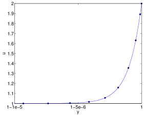
Figure 4.1: Solution of $(D^{2}-aD)u=0$ with $a=10^{6}$ and $u(1)=2$ and $u(-1)=1$. The figure shows the very thin boundary layer near $y=1$. The computed solution (solid line) is in excellent agreement with the exact solution (filled markers).

M1	M2	M3	node2	node3	error
16	1024	32	0.5	0.99999	5.80845e-06
16	4096	32	0.5	0.99999	4.07361e-11
32	128	32	0.999	0.99999	4.49718e-11
32	64	32	0.9999	0.99999	4.33247e-11
32	32	32	0.99995	0.99999	4.66069e-11

Table 4.1: Solution of $D^{2}-aD=0$ with $u(-1)=1$, $u(1)=2$, and $a=10^{6}$ using a grid with three intervals, which are discretized using $M1+1$, $M2+1$, and $M3+1$ Chebyshev points, respectively. Nodes 1 and 4 are located at $\pm 1$. Node 2 is outside the boundary layer in the first two rows. The error is in the infinity norm.

Table 4.1 summarizes spectral integration of piecewise Chebyshev grids applied to solve $(D^{2}-aD)u=0$ with $u(-1)=1$, $u(1)=2$, and $a=10^{6}$. This problem develops a boundary layer at $y=1$; see Figure 4.1. It is evident from the table, that the intervals must be chosen carefully. The table shows that attempts to get an accurate solution with fewer than a thousand grid points and just a single interval properly contained in the boundary layer did not work. The last row of Table 4.1 reports a solution with $M_{1}=M_{2}=M_{3}=32$ and an error of $4.7\times 10^{-11}$. In that computation, two intervals are contained inside the boundary layer. If a single Chebyshev grid is used, $M=8192$ is needed to get more than ten digits of accuracy.

The example of Table 4.1 coincides with Example 3 of [8]. Table 7 of [8] reports an error of $2.33\times 10^{-11}$ using $20$ intervals and $M=16$ for each interval (the total number of grid points is $321$).

4.2 An example with an internal layer

The second example we consider is $\epsilon u^{\prime\prime}+yu^{\prime}=0$ with boundary conditions $u(\pm 1)=\pm 1$ and $\epsilon=10^{-12}$. The exact solution of this boundary value problem is given by

$$u(y)=-1+\frac{2\int_{-1/\sqrt{2\epsilon}}^{y/\sqrt{2\epsilon}}{\rm e}^{-t^{2}}\,dt}{\int_{-1/\sqrt{2\epsilon}}^{1/\sqrt{2\epsilon}}{\rm e}^{-t^{2}}\,dt}.$$

The solution has an internal layer at $y=0$ of width approximately $\epsilon^{-1/2}$ or $10^{-6}$. In Figure 4.2, we show the spy plot of a matrix corresponding to division of $[-1,1]$ into five sub-intervals as well as the transition region of the solution.

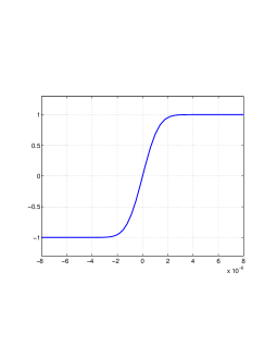
Figure 4.2: Solution of $u^{\prime\prime}+a\,y\,u^{\prime}=0$ with $u(-1)=-1$, $u(1)=1$, and $a=10^{12}$ using differentiation matrices and a piecewise Chebyshev grid. The plot shows the transition region of the solution.

m	node4	overshoot
32	$5\sqrt{\epsilon}$	3.7e-15
32	$3\sqrt{\epsilon}$	1.2e-08
32	$7\sqrt{\epsilon}$	8.6e-09
24	$5\sqrt{\epsilon}$	1.8e-08

Table 4.2: Solution of $\epsilon\,u^{\prime\prime}+y\,u^{\prime}=0$ with $u(-1)=-1$, $u(1)=1$, and $\epsilon=10^{-12}$ is shown in Table 4.2. This table gives the overshoot beyond $[-1,1]$ of the solution computed using 6 nodes and 5 intervals. Nodes 1, 2, 3, 5, and 6 are fixed at $-1$, $-8\epsilon^{1/2}$, $-3\epsilon^{1/2}$, $8\epsilon^{1/2}$, and $1$, respectively. The number of Chebyshev points in each interval is $m+1$.

This second example occurs near the end of [4], where it is reported that mapped Chebyshev points with $M=1024$ compute the solution with an overshoot of $3\times 10^{-4}$. From Table 4.2, we see that the overshoot is reduced to the order of machine precision using only $161$ grid points. The overshoot is seen to be highly sensitive to the location of the nodes. The solution plotted in Figure 4.2b corresponds to the top row of the table. The solution appears to have around $10$ digits of accuracy.

4.3 Differentiation errors and the Kleiser-Schumann algorithm

The two examples above are extreme examples of the efficacy of a piecewise Chebyshev grid. However, even in the application to the Navier-Stokes equation, a piecewise Chebyshev grid can give superior resolution with fewer grid points. Unfortunately, using a piecewise Chebyshev grid raises the CFL (Courant-Friedrichs-Lewy) number significantly and imposes an excessive constraint on the time step. Therefore, it does not prove useful. However, there are situations where the Navier-Stokes equations are solved for steady solutions and traveling waves without time integration [22]. Piecewise Chebyshev grids may prove useful in such applications.

The solution of the Navier-Stokes equation for channel flow or plane Couette flow involves two derivatives in the wall-normal direction. The first derivative arises when computing vorticities or the nonlinear term. The second order derivative arises when computing the right hand side of the pressure Poisson equation [20, 21]. Thus the rounding errors that arise during the differentiation operations may degrade the accuracy of the computed solutions.

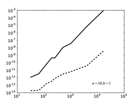
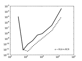
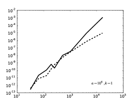
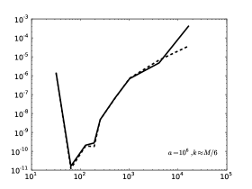
Figure 4.3: Plots of the infinite norm error in the derivative of $du/dy$ of the solution of $\left(D^{2}-a^{2}\right)u=f$ with boundary condition $u(\pm 1)=0$ against $M$, the number of Chebyshev modes. In the plots on the left, $f$ is chosen so that the exact solution is $u=\sin\pi y$. In the plots on the right, $f$ is chosen so that the exact solution is $f=\sin k\pi y$ with $k\approx M/6$. The dashed line corresponds to differentiation in the spectral domain without passing to the physical domain. The solid line corresponds to differentiation after passing to the physical domain.

Figure 4.3 shows differentiation errors in four different situations. In each case, the solution of $\left(D^{2}-a^{2}\right)u=f$ is computed using the method of Section 2.1 or 2.2. The difference between the solid line and the dashed line in the figure is minor. The derivative corresponding to the solid line is obtained by transforming the computed $u$ from Chebyshev space to physical space and then back to Chebyshev space for differentiation using the discrete cosine and sine transforms. For the dashed line, the computed $u$ is not transformed to physical space but is differentiated in Chebyshev space without going to physical space. In both cases, errors in the derivative are measured in the physical space.

The $a=10$ and $k=1$ plot corresponds best to the calculations in [14]. Here we see that the derivative obtained without passing to physical space is much more accurate. Most of the error is near the edges and the error would be lower in the energy norm. If $k\approx M/6$, the advantage of not passing to physical space is not as great.

The case $a=10^{6}$ is more relevant to turbulence simulations at high Reynolds number [20]. Here the advantage of not passing to physical space all but disappears, which is in agreement with the discussion in Section 3.3. Thus not passing to physical space appears to imply little advantage in turbulence simulation at high Reynolds number. In contrast, there is a significant gain in accuracy if numerical differentiation is avoided entirely by expanding $du/dy$ in a Chebyshev series as shown in [20].

The heart of the Kleiser-Schumann algorithm [13] for solving the Navier-Stokes equation in rectangular geometry is the following set of equations:

$$\frac{\partial u}{\partial t}+H_{1} =-\frac{il}{\Lambda_{x}}p+\frac{1}{Re}\left(D^{2}-\alpha^{2}\right)u$$

$$\frac{\partial v}{\partial t}+H_{2} =-\frac{\partial p}{\partial y}+\frac{1}{Re}\left(D^{2}-\alpha^{2}\right)v$$

$$\frac{\partial w}{\partial t}+H_{3} =-\frac{in}{\Lambda_{z}}p+\frac{1}{Re}\left(D^{2}-\alpha^{2}\right)w.$$

Here $2\pi\Lambda_{x}$ and $2\pi\Lambda_{z}$ are the extent of the domain in the wall parallel directions, and $u(y),v(y),w(y)$ are the coefficients of $\exp(il/\Lambda_{x}+in/\Lambda_{z})$ in the Fourier expansion of the velocity field. In addition, $\alpha^{2}=l^{2}/\Lambda_{x}^{2}+n^{2}/\Lambda_{z}^{2}$ and $H_{1},H_{2},H_{3}$ are nonlinear advection terms. The incompressibility condition is $(il/\Lambda_{x})u+\partial v/\partial y+(in/\Lambda_{z})w=0$. Using the incompressibility condition, we get an equation for pressure:

$$\left(D^{2}-\alpha^{2}\right)p=-\frac{il}{\Lambda_{x}}H_{1}-\frac{\partial H_{2}}{\partial y}-\frac{in}{\Lambda_{z}}H_{3}.$$

After time discretization, the Kleiser-Schumann algorithm solves these equations for the Chebyshev series of $u,v,w,p$. The type of errors discussed here occur when $H_{1},H_{2},H_{3}$ are computed for use in the next time step. In this computation, $u$ and $w$ are differentiated with respect to $y$. The nonlinear term $H_{2}$ is once again differentiated with respect to $y$ when solving for pressure.

The derivatives of $u,w$ with respect to $y$ may be formed without passing to the physical domain. Such an implementation would be more accurate at low Reynolds numbers, for which the parameter $a$ in $\left(D^{2}-a^{2}\right)u=f$ is small. But the advantage of not passing to the physical domain diminishes as the Reynolds number increases as evident from Figure 4.3.

5 Conclusions

In this article, we have derived many different versions of spectral integration for solving linear boundary value problems. The treatment of boundary conditions is uncoupled from finding a particular solution in each of these versions. As a result, the various forms of spectral integration can be combined in many ways.

The accuracy of spectral integration has a number of subtle features. In Section 3, we discussed the reason one can get away with not having to resolve boundary layers present in the Green’s function but not the solution as well as condition numbers and the accuracy of derivatives. The discussion is illustrated in Section 4 using numerical examples and motivates the new versions of Kleiser-Schumann and Kim-Moin-Moser algorithms derived in [20]. The new version of Kleiser-Schumann has been used to carry out a computation with $10^{9}$ grid points at $Re_{\tau}=2380$, which appears to be the highest Reynolds number reached in fully resolved simulations of wall bounded turbulence.

6 Acknowledgements

Thanks to Fabian Waleffe for comments and suggestions. Thanks as well to Hans Johnston and Benson Muite. This research was partially supported by NSF grants DMS-1115277 and SCREMS-1026317.

References

- [1] F.L. Bauer. Optimally scaled matrices. Numerische Mathematik, 5:73–87, 1963.
- [2] M. Charalambides and F. Waleffe. Gegenbauer tau methods with and without spurious eigenvalues. SIAM J. Numerical Analysis, 47:48–68, 2008.
- [3] M. Charalambides and F. Waleffe. Spectrum of the Jacobi tau operator for the second derivative operator. SIAM J. Numerical Analysis, 46:280–294, 2008.
- [4] E.A. Coutsias, T. Hagstrom, and D. Torres. An efficient spectral method for ordinary differential equations with rational function coefficients. Mathematics of Computation, 65:611–636, 1996.
- [5] T.A. Driscoll. Automatic spectral collocation for integral, integro-differential, and integrally reformulated differential equations. Journal of Computational Physics, 229:5980–5998, 2010.
- [6] D. Gottlieb and S.A. Orszag. Numerical Analysis of Spectral Methods: Theory and Applications. Society for Industrial and Applied Mathematics, 1977.
- [7] L. Greengard. Spectral integration and two-point boundary value problems. SIAM Journal on Numerical Analysis, 28:1071–1080, 1991.
- [8] L. Greengard and V. Rokhlin. On the numerical solution of two-point boundary value problems. Communications on Pure and Applied Mathematics, 44:419–452, 1991.
- [9] N.J. Higham. Accuracy and Stability of Numerical Algorithms. SIAM, Philadelphia, 2nd edition, 2002.
- [10] S. Hoyas and J. Jiménez. Scaling of the velocity fluctuations in turbulent channels up to = 2003 . Physics of Fluids, 18:011702(1–3), 2006.
- [11] S. Hoyas and J. Jiménez. Reynolds number effects on the Reynolds-stress budgets in turbulent channels. Physics of Fluids, 20:101511(1–8), 2008.
- [12] J. Kim, P. Moin, and R. Moser. Turbulence statistics in fully developed channel flow at low Reynolds number. Journal of Fluid Mechanics, 177:133–166, 1987.
- [13] L. Kleiser and U. Schumann. Treatment of incompressibility and boundary conditions in 3-D numerical spectral simulations of plane channel flows. In Proceedings of the third GAMM—Conference on Numerical Methods in Fluid Mechanics, pages 165–173, 1980.
- [14] B. K. Muite. A numerical comparison of Chebyshev methods for solving fourth order semilinear initial boundary value problems. J. Comput. Appl. Math., 234(2):317–342, 2010.
- [15] S. Olver and A. Townsend. A fast and well-conditioned spectral method. SIAM Review, 55:462–489, 2013.
- [16] S.A. Orszag. Galerkin approximations to flows within slabs, spheres, and cylinders. Physical Review Letters, 26(18):1100–1103, 1971.
- [17] S.A. Orszag and L.C. Kells. Transition to turbulence in plane Poiseuille and plane Couette flow. Journal of Fluid Mechanics, 96:159–205, 1980.
- [18] S.A. Orszag and A.T. Patera. Subcritical transition to turbulence in planar shear flows. In R.E. Meyer, editor, Transition and Turbulence, pages 127–146. Academic Press, 1981.
- [19] V. Rokhlin. Solution of acoustic scattering problems by means of second kind integral equations. Wave Motion, 5:257–272, 1983.
- [20] D. Viswanath. Navier-Stokes solver using Green’s functions II: Spectral integration of channel flow and plane Couette flow. www.arxiv.org, 1407.3776, 2014.
- [21] D. Viswanath and I. Tobasco. Navier-Stokes solver using Green’s functions I: Channel flow and plane Couette flow. Journal of Computational Physics, 251:414–431, 2013.
- [22] F. Waleffe. Homotopy of exact coherent structures in plane Couette flow. Physics of Fluids, 15:1517–1534, 2003.
- [23] A. Zebib. A Chebyshev method for the solution of boundary value problems. Journal of Computational Physics, 53:443–455, 1984.