Scanamorphos   : a map-making software for Herschel    and similar scanning bolometer arrays

Abstract

Scanamorphos is one of the public softwares available to post-process scan observations performed with the Herschel photometer arrays. This post-processing mainly consists in subtracting the total low-frequency noise (both its thermal and non-thermal components), masking high-frequency artefacts such as cosmic ray hits, and projecting the data onto a map. Although it was developed for Herschel, it is also applicable with minimal adjustment to scan observations made with some other imaging arrays subjected to low-frequency noise, provided they entail sufficient redundancy; it was successfully applied to P-Artémis, an instrument operating on the APEX telescope. Contrary to matrix-inversion softwares and high-pass filters, Scanamorphos does not assume any particular noise model, and does not apply any Fourier-space filtering to the data, but is an empirical tool using purely the redundancy built in the observations – taking advantage of the fact that each portion of the sky is sampled at multiple times by multiple bolometers. It is an interactive software in the sense that the user is allowed to optionally visualize and control results at each intermediate step, but the processing is fully automated. This paper describes the principles and algorithm of Scanamorphos and presents several examples of application.

withdrawn from A&A June 29, 2012 / submitted to PASP July 9 / report 1 received August 17 / re-submitted August 31 /
       referee 1 abandons / report 2 received November 19 / re-submitted November 30 / report 3 received February 19, 2013 /
       re-submitted April 3 / report 4 received July 11 / re-submitted July 26 / accepted July 27
       I have addressed 7 referee reports in total (including those from A&A) !

1 Introduction

The software described here was developed with the aim to process scan observations made with the photometers of the Herschel space telescope (Pilbratt et al. 2010), subunits of the PACS (Poglitsch et al. 2010) and SPIRE instruments (Griffin et al. 2010; Swinyard et al. 2010), but has broader applicability. Due to the mapping efficiency of the scan mode (also called on-the-fly mapping in ground-based astronomy) for fields larger than a few arcminutes, as opposed to the raster and jiggle modes, this is the preferred acquisition mode for extended Galactic regions, nearby galaxies and high-redshift surveys, in particular. Hence, scans are used extensively and represent a large fraction of the total observing time of Herschel, and the corresponding observing templates have been commissioned first. New observing templates based on very small scans have then been introduced after the Science Demonstration Phase to observe compact sources, in place of those based on chop-nod observations, that were found less sensitive.

During the course of a scan observation, the astronomical signal received by each bolometer is superimposed on a drift, occurring on timescales much longer than the sampling time interval. For small fields of view, the decontamination can be accomplished by chopping and nodding at frequencies higher than those characteristic of the drifts. This technique is not applicable to scan observations, and is appropriate only when reference positions devoid of emission from the target or background sources can be defined. The dual-beam scanning technique (Emerson et al. 1979), with a processing improved by Motte et al. (2007) to better remove atmospheric fluctuations, can be exploited to subtract only the thermal part of the drift, leaving the data contaminated by the non-thermal instrumental drifts. Simple scans with multiple detectors have the advantage of automatically providing the redundancy necessary to extract all the drift components, while spending all the time on source. A single scan already provides some level of redundancy, but most frequently at least two non-parallel scans are combined, ensuring that the drifts are well characterized (Waskett et al. 2007; Kovács 2008a), that transient signals can be suppressed, and that the desired sensitivity is achieved.

Low-frequency noise manifests itself most clearly by the presence of stripes in maps, oriented parallel to the scanning direction. But its removal is far from being only a cosmetic improvement, since this noise also decreases the sensitivity to low-brightness sources and alters the photometric and morphological source properties. It is natural to assign the task of removing low-frequency noise to the map-making module, because temporal and spatial information are interdependent and both necessary to characterize brightness drifts.

Several processing tools are available, within or outside the Herschel pipeline (HIPE; Wieprecht et al. 2009; Dowell et al. 2010; Ott 2010). Scanamorphos is a tool offered to the general user, coded in the Interactive Data Language (IDL), mainly for ease of programming and for the efficiency of multi-dimensional array processing that it affords. It is intended as an interactive tool, which means that users have the latitude to choose some map parameters and to visualize the results of intermediate processing steps. The algorithm principles are relatively intuitive and thus easy to understand. Its capabilities include the removal of additive brightness drifts caused by low-frequency thermal noise and flicker noise, the masking of cosmic ray hits left by the pipeline deglitching and of brightness discontinuities caused by glitches or electronic instabilities in PACS data, the projection of the data onto a spatial grid, and the production of the associated error and weight maps. The correction for all other instrumental effects is made beforehand by successive pipeline modules.

Bolometric imaging has been used extensively in the (sub)millimeter wavelength range, both on the ground or in balloons with medium and then large arrays and in space with single feedhorns, but Herschel and Planck are the first space missions to host bolometer arrays. Two different designs have been adopted for the photometer arrays of PACS (equiped with filters centered at 70, 100 and 160 $\mu$m) and for the photometer arrays of SPIRE (operating at central wavelengths of 250, 350 and 500 $\mu$m). The PACS arrays are composed of filled bolometer matrices, while the SPIRE arrays are made of pairs of bolometers and conical feedhorns, providing a sparse spatial coverage in staring mode. The instantaneous field of view is of the order of $3.5\arcmin\times 1.75\arcmin$ for PACS and $4\arcmin\times 8\arcmin$ for SPIRE. Bolometer arrays operating in the far-infrared and submillimeter domain contain increasing numbers of pixels and thus generate ever larger volumes of data. For Herschel, the number of bolometers per array varies between 43 (longest-wavelength SPIRE array) and 2048 (shortest-wavelength PACS array). As the algorithm described here makes use of the spatial redundancy built in the scan observations, the knowledge of the full history of all bolometers is needed at the same time, making the code a heavy consumer of computer memory for long observations. Extensive tests have been performed to determine memory specifications and execution times for given observation areas and depths (Sect. 5). For deep observations of very large fields, such as cosmology surveys, the software has the ability to automatically slice the field into several overlapping areas, that are processed successively and then mosaicked.

Scanamorphos requires only minimal knowledge of the instrumental characteristics for most of the processing, which should make it easily adaptable to other bolometer arrays. This was demonstrated by the results obtained with the ground-based P-Artémis instrument (André et al. 2008; Minier et al. 2009), the prototype of Artémis (Talvard et al. 2006), that will be fitted with filters centered at 200, 350 and 450 $\mu$m. Since its architecture is directly inspired from that of PACS, data acquired with P-Artémis were instrumental in testing and refining the code before the launch of Herschel. In all generality, however, the subtraction of the thermal low-frequency noise (atmospheric and instrumental) may require introducing additional noise terms that were not necessary for Herschel (see Kovács 2008b), and the observing strategy (scan pattern and sampling rate) has to be adequate for the chosen algorithm.

Sections 2 and 3 describe the principles and algorithm of the code. Section 4 presents the analysis of two PACS simulations to demonstrate the properties of Scanamorphos. Section 5 presents the results of tests performed on flight Herschel data, providing visual examples of operation. Appendix A gives an overview of the calibration of gain corrections for SPIRE, and Appendix B of the inputs and options of Scanamorphos. We conclude and give some practical details on the distribution in Sections 6 and 7.

2 Principles and prerequisites

Spatial redundancy is a general feature of scan observations. Within the portion of the sky observed with full coverage, each position is sampled by several bolometers, at many different epochs that are distributed over a large time interval. This provides an efficient means to remove brightness drifts without the need for chopped observations. Even though the redundancy built in standard scan observations with Herschel is minimal (a tiny fraction of the field is covered by any given bolometer), this is still sufficient to reconstruct brightness drifts accurately, as we shall demonstrate in this paper.

Since the power spectral density of the low-frequency noise has a broad overlap with that of real extended emission, and is therefore very difficult to determine empirically, Scanamorphos does not use any assumption in this respect. This is at odds with maximum-likelihood softwares based on matrix inversion, and more specifically MADmap (Ashdown et al. 2007; Cantalupo 2010), initially developed for cosmic microwave background experiments and implemented in the PACS and SPIRE pipelines. MADmap deals only with noise that is uncorrelated between detectors, assumes that the noise is Gaussian, piecewise stationary and circulant, and needs as input the noise spectral density, considered a stable calibration product (one per array), that has to be derived from deep observations of blank fields. In the event that the noise spectral properties are not accurately calibrated, vary with time or are altered by the pre-processing, then matrix-inversion algorithms will not produce optimal results, even though they update the noise properties by using an iterative approach. The effectiveness of a given class of algorithms will largely depend on the nature of the data and the acquisition mode. For pointed observations (as opposed to an all-sky survey), a modular and empirical approach, such as described by Kovács (2008b) for the CRUSH software (see also references therein), allows more flexibility: the signal can be weighted and masked as appropriate, without having to interpolate missing data, and other instrumental effects can be dealt with at optimal points along the processing chain, if necessary interleaved with the low-frequency noise subtraction. Another benefit of a software exploiting the redundancy is that it can be used to calibrate gains or flatfields from science observations, as shown in Appendix A.

In addition, the software ought to be able to process any data set containing both compact sources and extended structures on arbitrary spatial scales, while preserving their brightness distribution. Observations of nearby galaxies, or Galactic star formation regions, generate such data sets with a wide range of source characteristic lengths. With ground-based submillimeter instruments, extended emission is in practice extremely difficult to restore and to separate from the constantly varying atmospheric emission, unless more sophisticated observing strategies are designed. Simple scan observations performed on the ground are thus tailored to restore mostly compact or little-extended sources (i.e. smaller than the instantaneous field of view of the detector array). With space observatories, however, there is no such essential difference between compact and extended emission; the only contamination of the astronomical signal comes from the telescope and the detectors themselves, and since this noise varies on much longer timescales than atmospheric emission, it can be separated from the sky signal.

Herschel is not an absolute photometer, and all maps are therefore, at best, the superposition of an accurate representation of the sky and a global offset. The way of estimating the background level will in general depend on the exact astronomical application envisioned, especially in complex fields such as Galactic star formation regions, and should therefore not be determined by the map-making software, but by the map user.

Some other algorithms implemented in the Herschel pipelines are used extensively. PhotProject (for PACS) employs a high-pass filter. It is therefore useable only for compact sources, or else limited to subtract only the lowest-frequency component of the noise, so that extended emission will be filtered as little as possible. The Destriper (for SPIRE) performs the drift subtraction exclusively on the longest timescales, i.e. the same task as the subunit of Scanamorphos described in Section 3.4.

2.1 Important scan characteristics

During a scan observation, the telescope slews across the sky at approximately constant speed, while the detectors are read out at fixed time intervals, producing, after appropriate processing and calibration, samples of brightness as a function of time, with attached sky coordinates. We will hereafter refer to such brightness time series as simply “series”.

The scan pattern, i.e. the shape of the trajectory followed by the telescope, is indifferent for the subtraction of the drifts, except on the longest timescales of each scan (see Sect. 3.4), as long as it provides sufficient coverage and redundancy. A rectangular snake pattern is used for Herschel and P-Artémis, while a spiral pattern will be implemented for Artémis. Since there is often confusion between a scan and a scan leg (or subscan), that has to be lifted for the rest of this paper to be clear, we wish to emphasize the difference between them. A scan leg is a continuous segment of data acquired at constant scanning angle with respect to a fixed direction on the sky, and at constant speed. A scan is also a continuous segment of data, but comprises several parallel legs as well as the data acquired at non-zero acceleration while slewing from one leg to the next (turnaround data). It is best to have access to turnaround data whenever they exist in order to avoid edge effects. These data are indeed available for Herschel, but by default are not included in level-1 data for SPIRE (their inclusion requires the use of a dedicated option).

For the SPIRE instrument, the optimum scanning strategy, that is the basis of the default scan mode proposed to observers, is described by Waskett et al. (2007). For PACS, the choice of observing parameters such as the position angle of the arrays with respect to the scan direction is not as critical as for SPIRE, due to the fact that the arrays are filled. Constraints stemming from the array structure nevertheless exist (some position angles have to be avoided, because of the gaps between the subarrays).

Except for non-standard observations or preliminary reductions of incomplete datasets, at least two scans are combined for each field. The scanning directions should be separated by an angle of at least 20 degrees to ensure that the low-frequency noise is most efficiently separated from the astronomical signal (Waskett et al. 2007). The low-frequency noise series are in this case superposed to signal series that are intrinsically different in successive scans, making the two easier to disentangle.

The critical parameters for our purpose are the scan speed, the sampling rate and the onboard compression rate, that directly affect the available redundancy and the number of samples per beam crossing. The nominal scan speed is $30\arcsec/{\rm s}$ for SPIRE. For PACS, it is $20\arcsec/{\rm s}$. The fast scan speed of $60\arcsec/{\rm s}$, available for both instruments, should only be used for very large areas, as it does not ensure optimum redundancy and results in appreciably distorted point spread functions due to insufficient sampling (for PACS). The sampling rate of SPIRE is 18.6 Hz. Onboard compression is necessary for PACS, so as to be able to store and downlink the immense data volume generated by this instrument; from an initial sampling rate of 40 Hz, data frames are averaged to a final rate of 10 Hz. In parallel mode, in which both instruments acquire data simultaneously, the sampling rate is also 10 Hz for SPIRE and the red band of PACS (at 160 $\mu$m), but 5 Hz for the blue and green bands of PACS (at 70 and 100 $\mu$m).

For P-Artémis, the bolometer array has the same architecture as one PACS matrix (a filled square array with 16 pixels on a side), but the scanning strategy differs, especially in that it was chosen to offset the telescope by only a few arcseconds between two scan legs (about one pixel), making the available redundancy much higher, to increase the sensitivity. Simulations and flight acquisition of Herschel scans were therefore essential to test the robustness of the algorithm with respect to limited spatial redundancy.

The redundancy in each observation can be conveniently quantified by the coverage map or the weight map (see Sect. 3.7.1), excluding the edges. We shall take as unit of redundancy the number of samples per square FWHM per scan pair (the two scans having distinct orientations, most often nearly orthogonal). The redundancy depends on the structure and position angle of the array with respect to the scan direction, on the separation between adjacent scan legs, on the scan speed and sampling rate. For the Herschel observations presented as illustrations in Section 5, it varies between 75 and 530. Nominal SPIRE observations at $30\arcsec/{\rm s}$ have redundancies of 150 to 180, with $3\sigma$ dispersions of 30 to 40% . Nominal PACS observations at $20\arcsec/{\rm s}$ have redundancies of 350 (at 70 $\mu$m) to 530 (at 100 $\mu$m), with $3\sigma$ dispersions of 35 to 55% . For the PACS blue and green bands in parallel mode, it is divided by two, thus on the same order as for nominal SPIRE observations. With a pixel size equal to the default for the final projection, i.e. FWHM/4, this fiducial value translates to about 10 samples per pixel per scan pair.

2.2 Low-frequency noise

The low-frequency noise has two main components. A first part comes from small temperature fluctuations of the cryogenic bath. As the bath temperature varies coherently across the array, these fluctuations produce for each bolometer a noise that is strongly correlated with the noise of the other bolometers. In principle, this noise is calibratable for SPIRE, because the arrays contain some thermistors and blind bolometers that can be used as temperature probes, unaffected by temperature variations due to the sky signal. In practice, however, the thermal drifts have other dependencies that are currently not accounted for in the parameterization that is used to correct for them in the pipeline. The option to choose one or the other method does not exist for PACS, that lacks blind detectors, so the removal of correlated noise by the map-making software is a genuine necessity for this instrument.

The second component, that can be assimilated to flicker noise, is non-thermal and uncorrelated from bolometer to bolometer. It is determined by detector physics and readout electronics and cannot be calibrated. The knee frequency is defined as the frequency where the power spectral density of the flicker noise is equal to that of the white noise. In laboratory tests and flight operations, it has been measured to be less than 0.1 Hz for SPIRE (Griffin et al. 2010), but more than 1 Hz for PACS (Poglitsch et al. 2010).

The brightness drifts are expected to come only from these two sources of noise and therefore to be purely additive. It is assumed that multiplicative instrumental effects such as gains and flatfields are perfectly stable, which was so far verified.

2.3 Pre-processing and interface with the Herschel pipeline

In the Herschel data processing chain, map-making utilities take as input level-1 data (flux-calibrated time series with the associated pointing information) and produce level-2 data, i.e. maps with all instrumental effects removed as well as possible. The pre-processing by the pipeline includes the following steps (not mentioned here in their actual order): 1) from level 0 to level 0.5, bad channels are masked and samples with underflow/overflow are flagged, ADUs are converted to voltages and times are attached to each sample; from level 0.5 to level 1, the pointing of each bolometer is computed, the data are deglitched and converted to brightnesses (in Jy per beam for SPIRE or Jy per array pixel for PACS), corrections are made for electrical and optical crosstalk, for the electrical filter response and the bolometer time response, and, for SPIRE only, the thermal drifts are subtracted by using the smoothed series of thermistors located on the detector array as inputs to a drift model.

When post-processing SPIRE data with Scanamorphos, it is possible to bypass the thermal drift correction within the pipeline, since this correction is also dealt with by Scanamorphos. Below, a comparison is made between the results from the two algorithms, to demonstrate the usefulness of Scanamorphos in removing thermal drifts in both instruments. Users are encouraged to compare both approaches and to select the most effective for their data, or possibly to use the Scanamorphos module coping with thermal drifts as a second-order correction, if the redundancy is very limited (i.e. if the observation consists of only one scan or two scans).

Before correcting for the low-frequency noise, another pre-processing step is necessary for Herschel data. The conversion of the voltage of each bolometer to an in-beam flux density is made with reference to a fixed voltage, representing what would be measured on a perfectly dark sky in the same conditions as those of the observation. In practice, this fixed voltage cannot be accurately calibrated, which means that the signal of each bolometer is the superposition of the true sky signal, the noise, and a large offset (varying strongly from bolometer to bolometer). These offsets are removed within Scanamorphos as part of zero-order baselines (one constant per bolometer per scan leg is derived). The constants are computed so as to be minimally contaminated by both extended and compact sources; but any small error in their determination can be corrected afterwards by a linear baseline removal module making use of the redundancy instead of simple fits (i.e. a destriper; see below). The pipeline also includes a module dealing with these offsets and performing either baseline subtraction or high-pass filtering (between levels 1 and 2), and it is strongly recommended to bypass it in view of a subsequent Scanamorphos processing.

Level-1 data can be accessed outside the pipeline by first saving them on disk in Flexible Image Transport System (FITS) files (Wells et al. 1981; Hanisch et al. 2001), with a format specific to Herschel, and then converting these files with an IDL utility to a format readable by the map-making software. The conversion utility is included in the Scanamorphos tree.

Invalid bolometers are rejected by this data formatting task. The SPIRE 250 $\mu$m array contains a total of 139 detectors (7 always de-activated), the 350 $\mu$m array 88 detectors (1 always de-activated), and the 500 $\mu$m array 43 detectors (1 always de-activated).

The PACS blue array (operating at 70 and 100 $\mu$m) contains 2048 pixels, and the red array (operating at 160 $\mu$m) 512 pixels. They also contain a very small fraction of dead pixels. In addition, for a few rows of the blue array, the signal is seen to oscillate between an upper state and a lower state. This is caused by electronic instabilities in the multiplexing circuit. The few 16-pixel blocks that are the most frequently affected by such artefacts have been identified from a database of nearby galaxy observations, and are entirely masked before the processing begins.

3 Algorithm

3.1 Overview

Our algorithm does not strictly speaking separate the low-frequency noise into thermal and non-thermal components, since it cannot discriminate between different physical origins. It uses a different but mathematically equivalent decomposition: the thermal noise is replaced with the average noise (the same time function for all bolometers), and the flicker noise by the complement (an independent time function for each bolometer). This alternative decomposition is easier to handle algorithmically. We also make a practical distinction between long-timescale and short-timescale drifts, but only because they are subtracted by different means.

Here are the main computations and corrections performed in sequential order:
1) computation of map coordinates from sky coordinates; optionally slicing of the dataset into several spatial blocks (for very large data volumes; see Sect. 3.8)
2) computation of scan speed as a function of time and tagging of nominal data and non-zero acceleration data (on the edges of the map); masking of scan speed anomalies due to position errors
3) computation of space and time grids adapted to the drift subtraction problem (Sect. 3.2)
4) division of the signal by the relative gains (SPIRE only; Appendix A)
5) computation of high-frequency noise (Sect. 3.3)
6) subtraction of linear baselines, effectively removing brightness drifts with timescales comparable to or larger than the scan leg duration (Sect. 3.4); and, for PACS only, masking of brightness discontinuities (see Sect.3.6.1)
7) update of high-frequency noise, first-pass glitch masking (Sect. 3.6.2), and detection of asteroids (Sect. 3.6.3)
8) subtraction of the average drift (on timescales smaller than the scan leg duration) and residual glitch masking (Sect. 3.5.1, 3.5.2 and 3.6.2)
9) subtraction of individual drifts (on timescales smaller than the scan leg duration) and residual glitch masking (Sect. 3.5.3 and 3.6.2)
10) projection of signal, error, total drifts and weight maps on a fine pixel grid (Sect. 3.7)
11) optionally mosaicking of the spatial blocks processed separately (Sect. 3.8).

In what follows, it is unavoidable to mention some of the software options in order to highlight some branch points of the algorithm. They are presented in Appendix B.

3.2 Spatial and temporal grids

To determine drifts from redundant data, the underlying principle is the following: at a given position on the sky, the astronomical signal received by the detectors is the same at any time, and the signal read out from various bolometers at various times differs only by the low-frequency noise affecting the detectors at these particular times plus the high-frequency noise (that includes glitches, physical white noise and quantization noise, also white):

$$R(t,b_{i})=G(b_{i})\times S(p)+LF(t,b_{i})+HF_{0}(t,b_{i})$$ (1)

where $R(t,b_{i})$ is the signal recorded at time $t$ by the bolometer $b_{i}$ , $S(p)$ is the sky brightness in the pixel $p$ sampled by $b_{i}$ at time $t$, the gain $G(b_{i})$ is the relative beam area of bolometer $b_{i}$ (for SPIRE only; see Appendix A), $LF(t,b_{i})$ the total low-frequency instrumental noise affecting bolometer $b_{i}$, and $HF_{0}$ the high-frequency noise. Defining the average drift as  $\bar{D}(t)=\frac{1}{N_{b}}\sum_{i=1}^{N_{b}}\frac{LF(t,b_{i})}{G(b_{i})}$  (where $N_{b}$ is the number of valid bolometers) and the individual drift of bolometer $b_{i}$ as  $D_{b_{i}}(t)=\frac{LF(t,b_{i})}{G(b_{i})}-\bar{D}(t)$  we obtain

$$R(t,b_{i})/G(b_{i})=S(p)+\bar{D}(t)+D_{b_{i}}(t)+HF(t,b_{i})$$ (2)

where the new $HF$ term is simply the original high-frequency noise divided by the gain. Our decomposition of the low-frequency noise allows us to ignore any differential gains between signal and noise, as long as they are constant.

It is then necessary to define precisely the finite region of the sky within which the intrinsic signal will be considered uniform, to compare all the samples taken within this region and derive the drifts from them. Ideally, this region should be much smaller than the point spread function to avoid distorting compact sources. In practice however, the sampling rate is too limited to provide sufficient statistics within regions smaller than the beam FWHM; another consideration to take into account is the efficiency of the code in terms of execution time. We thus adopt the beam FWHM as the spatial scale of signal invariance in our drift removal procedure. In this case, a way to detect and protect compact sources has to be implemented. In addition, we must ensure that the low-frequency noise is stable during the time needed to cross this region.

Since the flicker noise becomes smaller than the white noise above a knee frequency, a limiting timescale can be defined below which its effects will be negligible and impossible to correct. This timescale should be longer than the beam FWHM crossing time to obtain an optimal correction. For the SPIRE bands at 250, 350 and 500 $\mu$m respectively, at the nominal scan speed of 30 arcsec s^-1, the FWHM corresponds to minimum timescales of 0.6, 0.8 and 1.2 s, or maximum frequencies of 1.7, 1.2 and 0.8 Hz. Laboratory measurements of the SPIRE noise knee frequencies are all well below these limits, of the order of 0.1 Hz. For the PACS bands at 70, 100 and 160 $\mu$m, at the nominal scan speed of 20 arcsec s^-1, the minimum timescales are about half those of SPIRE, 0.28, 0.34 and 0.57 s, corresponding to maximum frequencies of 3.6, 2.9 and 1.8 Hz. The PACS noise knee frequencies are of the order of 1 Hz or higher, for all applied polarization voltages tested in the laboratory (Billot 2008). Then, in practice, the knee timescale may be shorter than the beam FWHM crossing time in some configurations for PACS (see below).

We thus define two spatial grids during the processing: a grid for mapping, with a pixel size equal to half the beam FWHM by default, and a coarse grid for drifts removal (for steps 8 and 9 in Sect. 3.1), with a pixel sized by the beam FWHM by default, i.e. our chosen stability length. The algorithm uses an iterative process, and a map using the latest drift correction is projected onto the mapping grid before each iteration. Then, at the end of the processing, the data are projected onto a final grid, with a default pixel size set to a fourth of the beam FWHM (changeable by the user).

We require at least 6 samples per stability length $l_{s}$ to enable the computation of simple statistics. The sampling rate is too low in some cases to meet this requirement with a stability length of FWHM (for PACS, or for SPIRE in parallel mode). The pixel size of the coarse grid is automatically increased if needed, in increments of FWHM/2. The coarse spatial grid is in fact duplicated after offsetting it by half a pixel in each coordinate, to provide better sampling of the drifts.

Similarly, two temporal grids are used during the processing: the native grid corresponding to the sampling times, and a coarse grid adapted to the drifts computation. The time step of the coarse grid is the crossing time of the stability length defined above: $T_{c}~{}=~{}l_{s}~{}/~{}v_{\rm scan}$, where $v_{\rm scan}$ designates the scan speed, which defines the coarse time grid: $t_{c}~{}=~{}k~{}T_{c}$, $k=0,1,...,n_{c}$.

In unfrequent cases, and when the spatial grid makes an angle close to $45^{\circ}$ with a scan direction, it was noticed that the subtraction of the low-frequency noise did not perform optimally, leaving some residual short-timescale striping. This may be due to the fact that in this configuration, a larger fraction of the data is unusable for the drifts computation, since bolometers scanning a pixel corner, instead of crossing a pixel along a diagonal or a side, are rejected for lack of sufficient statistics. Because it is not possible to predict if a given orientation will be unfavorable for the drifts subtraction or not, all the processing is systematically done in the optimal orientation determined by the code (e.g., for the simplest case of observations made of orthogonal scans, with the x axis parallel to the direction of the first scan). The spatial grid chosen by the user is enforced only for the final projection.

3.3 High-frequency noise

The high-frequency noise standard deviation serves as a benchmark to quantify the low-frequency noise amplitude, and to weight the data by its inverse square. It is measured, for each bolometer and each scan, from the binned average of the spectral density between 2.5 and 5 Hz for SPIRE (where spectral densities reach a plateau), and between 3 and 5 Hz for PACS (for which the true white noise cannot be estimated, since spectral densities do not reach their minimum at 5 Hz). For convenience, we call these estimates “white noise”, although this is an inaccurate designation in the general case.

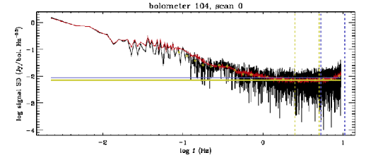
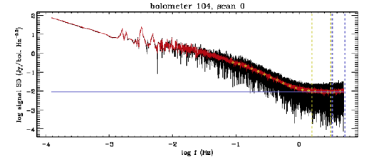
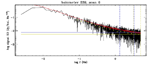
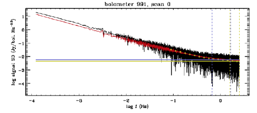
Figure 1: Example of determination of the high-frequency noise from spectral densities computed after interpolating compact sources and glitches, at the nominal SPIRE sampling rate (top left, from the NGC 6946 250 $\mu$m observation), at the parallel-mode sampling rate for SPIRE (top right, from the Rosette 250 $\mu$m observation); and for PACS in nominal mode (bottom left, from the NGC 4559 160 $\mu$m observation), and in parallel mode for the blue array (bottom right, from the Rosette 70 $\mu$m observation). SD stands for spectral density, and f for frequency. The vertical lines show the frequency ranges within which the average of the spectral density is computed, and the horizontal lines the derived noise spectral density. The white noise is coded in yellow, and the threshold noise in blue (see Sect. 3.3). The yellow diamonds represent the binned spectral density. The high-frequency noise is computed individually for each bolometer. The red curve shows the average spectral density of all bolometers, for comparison.

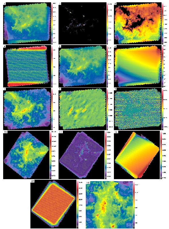
Figure 12: Successive steps of the processing of the Rosette 250 $\mu$m observations illustrated by maps, showing the following: 1) raw level-1 data; 2) signal of compact sources interpolated for the computation of high-frequency noise; 3) mask applied for the computation of baselines; 4) simple baselines obtained by zero-order fits (since the /galactic option is used); 5) data after subtraction of the simple baselines; 6) residual baselines derived from the redundancy; 7) data after subtraction of the residual baselines; 8) average drift subtracted at the first iteration; 9) individual drifts subtracted at the first iteration for these; 10) final map; 11) error map; 12) total drifts (dominated by baselines); 13) weight map; 14) enlargement of a central portion of the final map (about $50^{\prime}$ on a side). Notice the very different brightness scales for the signal and for the drifts. Maps 1 to 9 are projected on a coarse spatial grid (with a pixel size equal to half the stability length), and maps 10 to 14 are projected on a fine grid (with pixels of FWHM/4 on a side). The final map shows a wealth of filamentary structures at various spatial scales, and compact sources, with no sign of residual striping.

Prior to the computation of spectral densities, real high-frequency signal - that may contaminate our noise estimates - is masked in the following way: whenever the absolute difference between the signal at a given time and the signal between one and three time steps later exceeds a given threshold (computed from the dispersion of the absolute differences in the observation), a total interval of six samples around that time are temporarily masked out. Because the Fourier transform needs continuous time series, the masked samples are then interpolated, and an artificial Gaussian noise is added to the interpolates. The mapping of the signal that has been removed in this way shows that the procedure is effective at removing both bright compact sources and glitches (an example is shown in Fig. 12).

For the removal of drifts, it is necessary to use a second noise quantification that serves to define a threshold for the detection of compact sources, steep brightness gradients and glitches (see Section 3.5.1). For SPIRE, since some pipeline modules using Fourier transforms amplify the high-frequency noise, the spectral densities rise again beyond 5 Hz. To take this into account in our noise threshold, we measure the average noise standard deviation between 5 and 10 Hz. We call this estimate (or the “white noise” estimate if it is larger) the “threshold noise”. Similarly, we measure such a quantity for PACS, between 1.3 and 3 Hz. All the frequency windows are modified in parallel mode, when the sampling rate is lower. Illustrations of the high-frequency noise computation are shown in Fig. 1. After computing the high-frequency noise of all bolometers, in each scan, those with very deviant noise values are masked and not further used.

For PACS, the brightness quantization noise is in some cases a significant fraction of the high-frequency noise. We estimate it in the following way: for each bolometer and each scan, the quantization step $q$ is defined as the minimum brightness where the histogram of $|B(t_{i+1})-B(t_{i})|$, computed on a very fine brightness grid (excluding zero), is populated, $B(t_{i})$ being the brightness recorded at the $i^{\rm th}$ time sample. Assuming that the quantization error is uniformly distributed between 0 and $q$, the quantization noise variance is then $q^{2}/3$. When this term dominates the high-frequency noise (which happened in the early stages of the mission when using a very low gain), it may limit our ability to subtract the low-frequency noise down to acceptable levels.

3.4 Long-timescale drift subtraction

Scan observations do not allow to separate the brightness drifts from the signal on spatial scales similar to or larger than the map size, i.e. on timescales of the order of the scan leg duration of larger. Such drifts, if left uncorrected, may introduce artificial brightness gradients. For thermal drifts, that are usually coherent over the duration of several scan legs or whole scans, these gradients will be perpendicular to the scan direction (see an example in Sect. 5.2.2). The simplest way to remedy this problem is to subtract linear baselines, computed either on a scan basis, or on a scan leg basis, but this requires particular care, in order to keep the baselines immune to real structures that are smaller than the field of view, and to preserve as much as possible brightness gradients that could be real. These baselines in fact cover several distinct instrumental artefacts: the primary component consists of flux calibration offsets, as mentioned above (Sect. 2.3), and the rest comprises the long-timescale component of both the thermal drift and the flicker noise.

We argue that baselines should not assume the form of polynomials of any order higher than 1 (this is an option offered in the pipeline), whenever possible. With an order of 2 or higher, the shape of structures smaller than the field of view is altered, in an uncontrolled way. In Scanamorphos, the subtraction of the drifts on timescales smaller than the field of view crossing time are left to specific modules using the redundancy, and thus operating in a controlled way, such that flux and morphology are conserved.

The baseline-subtraction algorithm described here was implemented specifically for Herschel, and needs to be adapted if scans cannot be sliced into distinct scan legs. We need to distinguish three categories of fields, for which the algorithm will be slightly different. Extragalactic fields are the easier case, because the sky has at most very mild brightness gradients, that are insignificant with respect to the effects of a thermal drift (any field where a flat sky can be isolated from sources belongs to the same category, even if located within the Galaxy). The second case is that of bright Galactic fields (e.g. star formation regions), where sky gradients can become comparable to the artificial gradients induced by the drifts; their separation requires special steps. Finally, another modification to the general algorithm is needed for very small fields, as explained at the end of this section.

Extragalactic or faint fields:

First, simple baselines are computed by the process outlined below in points 1 to 3, iterated three times:
1) On a scan basis, we fit a linear function to the signal averaged over all valid bolometers, and subtract it from the signal of each bolometer. In practice, this removes a major part of the average low-frequency noise. This step can modify the general brightness gradient in the scan-perpendicular direction, but not in the scan-parallel direction.
2) On a scan leg basis, one offset (or zero-order baseline) is subtracted for each valid bolometer. This step takes care of flux-calibration offsets, and can also include a very small contribution from the low-frequency noise, since the offsets are allowed to vary from one scan leg to the next. Each offset is determined as the median of the series.
3) At the third iteration, zero-order baselines in step 2 are replaced with linear baselines. A distinction is made between fields with structure extending over scales similar to the map size, and fields where the extended emission is confined to the central part of the map: if the former case applies, then the baselines are constrained such that their average over all valid bolometers reduces to the zeroth order, so that in practice the general brightness gradient is not altered. An example of such a case is a field with strong cirrus emission on one side of the map (see Sect. 5.1.3).

The fits in steps 1 and 3 and the offsets in step 2 are robust, in the sense that a mechanism is in place to iteratively exclude sources from the brightness series, both in the time domain and in the spatial domain. For the latter, a new map is created after each step, and sources above a given threshold are masked; the mask is then transferred to the time domain. The applied brightness threshold is determined automatically, and is chosen so as to avoid masking predominantly the edges, in case significant structure exists outside the central part of the map (see an example in Sect. 5.1.1).

The discrimination between the two types of structure in step 3 is made automatically, and requires no user input. It is based on the same source mask as above, except that the brightness threshold is fixed. The map is divided into a central part (one ninth of the surface area) and the periphery. The fractional area of the source mask located within the central part decides of which case applies: if it is smaller than a given threshold, and if the total area of the mask is significant, then we consider that there is extended emission throughout the map.

4) Once these simple baselines are subtracted, they are refined by using the redundancy in the observation instead of fits (which provide a useful pre-correction but are unphysical). This complementary destriping ensures that the most accurate solution is found, by minimizing the deviations between different bolometers and between successive scans. This is an iterative process using the same source mask as above. At each iteration, and for each scan leg, the difference between the series of each valid bolometer and the series simulated from a reference map (both associated with the same sky coordinates) is computed and fitted by a linear function, and this linear baseline is subtracted from the data; then the map is updated and the process repeated until convergence. The reference map is first built from scans taken in the direction orthogonal to the scan leg under consideration, and then in later iterations from all scans (see below for a detailed explanation).

The destriping algorithm assumes that each scan leg is separated from the next by a spatial offset larger than the FWHM or a few times the FWHM. While this is always true for nominal observations, this condition is not verified for fine scans used for calibration purposes. When processing fine scans, the destriping module should therefore be deactivated.

Galactic or complex bright fields:

For observations of such fields, if the relevant option is used (/galactic), the baseline subtraction is modified with the aim to protect as well as possible complex structures of0.3ten extending over much larger scales than the field of view. The modified algorithm is applicable only when sources are bright enough to be visible in the map built from raw data (or rather when only the flux calibration offsets have been subtracted).
1) On a scan basis, linear baselines are replaced with simple offsets, so that the natural brightness gradients of molecular clouds, usually dominant over gradients induced by low-frequency noise, are left intact. The offsets are computed for each valid bolometer as the median of the series, and in practice eliminate the flux calibration offsets.
2) Still on a scan basis, linear baselines are computed by using the redundancy: the difference between the average series of the valid bolometers and the average series simulated from a reference map is computed and fitted by a linear function, and this linear baseline is subtracted from the data; then the map is updated and the process repeated for a total of four times. For each scan, the reference map is built from the scans acquired in the (near-)orthogonal direction only, in the first two iterations. In the last two, once the scans have been rectified, the reference map includes all the scans. Natural gradients are preserved for this reason: when subtracting a linear baseline from a whole scan, only the gradient perpendicular to the scan direction can be modified; any gradient parallel to the scan direction would create a periodic signal (with a period equal to the duration of two scan legs), and would not create any linear component. Any real gradient will be present in both the fitted scan and the reference map, and thus cancelled when subtracting the series simulated from the reference map, before doing the fit. As to the artificial gradients caused by the thermal drift, they are to first order perpendicular to the scan direction (i.e. parallel to the displacement from one scan leg to the next), since low frequencies are dominant. Thus they have a distinct orientation in the fitted scan and in the reference map, when the latter is built from scans acquired at a sufficiently distinct angle: the drift in a given scan will be left intact by the subtraction of the reference series and can be fitted by a linear function and removed.
3) The destriping is repeated, this time for each bolometer independently, on smaller segments of four scan legs, i.e. at a better time resolution but still ensuring immunity to scan-parallel gradients. The scheme to build the reference map is the same as in step 2.
4) Then, the destriping on a scan leg basis is made in the same way as for extragalactic fields.
A source mask is also defined and used in the same way as above in all steps.

Very small fields:

For such observations, the destriping and average drift subtraction on small scales become impossible, because there are not enough resolution elements across the map. This can lead to an ill-determined thermal drift, in case it is significantly non-linear, which occasionally happens. To solve this problem, for small fields whose source mask covers a small fraction of the total area, we allow third-order baselines in place of linear baselines (on a scan basis). The order change is however effected only when the new fit is of much better quality than the linear fit, as measured by the $\chi^{2}$ value.

3.5 Short-timescale drift subtraction

We now discuss the removal of drifts on timescales shorter than the scan leg duration, which can be derived without any assumptions on the sky structure, contrary to those discussed in the previous section.

3.5.1 Average drift

In a first step, as mentioned in Section 3.1, thermal drifts are considered to be uniform over the whole array; any component that differs from the average is treated in the second step, as part of the uncorrelated drifts. We thus have to determine a single series for the thermal noise.

For each pixel of the coarse grid (Sect. 3.2), all the samples recorded while the beam center lies within this pixel are searched; an efficient IDL function is used to perform this task quickly and store the sample indices beforehand. Then, the samples are divided into separate bolometer crossings, for each of which the brightness mean and the brightness mean absolute deviation are computed, and to each of which an average time is attached. Bolometers scanning only pixel corners, with insufficient statistics, are discarded.

At this point, the presence of a compact source, a steep brightness gradient, or an abnormal level of high-frequency noise within the pixel, is tested in a straightforward way: if the mean absolute deviation of a bolometer crossing is below the average threshold noise of this bolometer (defined in Section 3.3), then it is deemed suitable for drift determination; otherwise, the assumption of a uniform astronomical signal is not valid. We then distinguish two cases: 1) If more than 70 to 80% of the bolometer crossings are suitable for drift computation, then they are effectively used, and only those bolometer crossings with an elevated mean absolute deviation are discarded. 2) In the opposite case, then a significant portion of the coarse pixel area is assumed to contain non-uniform signal, and all the bolometer crossings are discarded. If the sampling rate allows the statistics to remain sufficient at smaller scales, then the algorithm switches to a finer spatial grid, to which the same test is applied; if the test is again negative, all the bolometer crossings are again rejected.

The measured brightness difference between each pair of suitable bolometer crossings is in principle equal to the difference of the drifts between the two sampled times. Calling the first bolometer $b_{i}$, crossing the pixel $p$ at the average time $t_{1}$, and the second bolometer $b_{j}$, crossing $p$ at the average time $t_{2}$,

$$\delta(t_{1},t_{2})=R(t_{1},b_{i})-R(t_{2},b_{j})$$

$$=\bar{D}(t_{1})-\bar{D}(t_{2})+D_{b_{i}}(t_{1})-D_{b_{j}}(t_{2})+HF(t_{1},b_{i})-HF(t_{2},b_{j})$$

The $S(p)$ term in Equ. 2 cancels because the astronomical signal is assumed both invariant in time and uniform within $p$, making the different trajectories of $b_{i}$ and $b_{j}$ within $p$ irrelevant. The software is in fact able to cope with mild non-uniformity within $p$, since the current map is used to cancel, whenever possible, brightness differences purely caused by small pointing differences, as explained in Section 3.5.4. Then, by linear interpolation, $\delta(t_{c1},t_{c2})$ (on the coarse time grid defined in Section 3.2) is obtained from $\delta(t_{1},t_{2})$ .

Each term $\delta(t_{c1},t_{c2})$ is stored in a matrix where the first dimension represents the smaller of the two times, and the second dimension the larger. Drift differences are coadded in this matrix as they are computed, regardless of the position on the sky or the bolometers involved. Their weights, inversely proportional to the square white noise of each bolometer, are stored symmetrically across the matrix diagonal. This ensures, together with the use of a coarse time grid adapted to the minimum drifts timescale, that memory usage is minimized.

One obtains by coadditions

$$\delta(t_{c1},t_{c2})=\bar{D}(t_{c1})-\bar{D}(t_{c2})+{\rm WM}_{p,i,j}~{}[D_{b_{i}}(t_{c1})-D_{b_{j}}(t_{c2})]$$ (4)

where WM designates the weighted mean and the sum runs on all pixels $p$ and all pairs of bolometer indices ($i$, $j$) such that $b_{i}$ is crossing $p$ at time $t_{c1}$ and $b_{j}$ is crossing the same pixel $p$ at time $t_{c2}$. The high-frequency noise term rapidly vanishes and, given that the individual drifts are all independent of each other, the WM term above also becomes negligible if the redundancy is sufficient. Taking as an example the 70 $\mu$m PACS observations of the Rosette nebula discussed in Section 5.2.2, made of 2 scans in parallel mode at the scan speed of $20\arcsec/{\rm s}$ (thus with relatively low redundancy), the median number of contributing bolometer crossings for a given ($t_{c1}$, $t_{c2}$) time pair is $N_{\rm coadd}\simeq 380$ , with a very large spread. The residuals of the WM term in $\delta(t_{c1},t_{c2})$ are thus of the order of $\frac{1}{\sqrt{N}_{\rm coadd}}\simeq 5$% of the average amplitude of the individual drifts (which is larger than the amplitude of the average drift at any given frequency for PACS). However, the average drift series is obtained from the $\delta(t_{c1},t_{c2})$ terms in a complicated fashion (see next section), involving many more coadditions. Although a rigorous analytic estimate cannot be made, the final residuals due to the WM terms are very small compared with the amplitude of the average drift, as proven by the simulations in Section 4. Let us remark that the probability law of the individual drifts does not have to be assumed Gaussian; it only has to be symmetric about zero. Finally, $\delta(t_{c1},t_{c2})\simeq\bar{D}(t_{c1})-\bar{D}(t_{c2})$.

Once all pixels have been covered, the matrix is read so as to restore from the drift differences the average drift series (see next section), that is subtracted from the signal series of each bolometer. Since it is impossible to define the absolute zero of the drift, it is previously offset so that its time average is null. Then a new map is projected.

This process is iterated until convergence, which is reached when the drift amplitude has become smaller than the white noise level for most bolometers. Here, the amplitude of the drift is defined as three times its standard deviation.

3.5.2 From drift differences to the absolute drift series

The conversion of the drift differences matrix to the absolute drift series is not trivial. First, the matrix is scanned several times in each direction, progressively populating the drift series. One entry time is chosen and arbitrarily assigned a null drift. Then, each drift difference between two times of which one has already an entry in the drift series is used to assign an absolute drift to the second time index. At the same time as the drift series is built, a corresponding weight series is computed, and used to weight appropriately the drifts as they are coadded. The matrix is scanned until the drift series converges.

This process does not provide a unique solution. Let us assume that the average drift $\bar{D}(t)$ is replaced with $\bar{D}(t)+E(t)$, where $E(t)$ is an excess drift, such that the projection of this series produces the same map for each successive scan (i.e. $E(t)$ is an oscillatory function, with a period equal to that of the spatial coordinates, just like the average true sky series). Then the $\delta(t_{1},t_{2})$ term in Equation 3.5.1 is unchanged, because it is computed within a single pixel $p$, where $E(t_{1})$ and $E(t_{2})$ take the same value. The drift series obtained by scanning the drift differences matrix is thus the superposition of the true drift series and an oscillatory component. The average drift has no reason to repeat itself exactly in successive scans. We thus extract this periodic component from the average drift and remove it, before subtracting the average drift from the data. This is achieved by first mapping the average drift for each scan separately, and extracting the component common to all these maps, that we call the excess drift. Then, the series of the excess drift is simulated from its map, and finally subtracted from the original drift.

We now briefly explain the method used to extract the excess drift from the drift maps. This method has to provide reliable results even when the observation is composed of only two scans, i.e. only one period of the excess drift. We exploit the fact that, by definition, the excess drift varies on much longer timescales than the true drift (that varies on timescales shorter than the duration of a scan leg). This implies that the spatial variations of the excess drift in the drift maps are much smoother than those of the true drift. For each drift map (one per scan), a map of the local variance is computed (using as zero moment a boxcar-averaged version of the drift map). Then the excess drift map is defined as the weighted average of all the drift maps, the weight for each one being the inverse variance map. Obviously, the error on the excess average drift will go down as the number of scans increases. When a large number of scans are combined, the excess drift map is simply defined as the median of all the drift maps.

3.5.3 Individual drifts

In a second step, the individual drifts are removed. At this stage, by definition, the drift affecting the average signal of all valid bolometers should be close to zero at all times. Using the same scheme as previously and protecting non-uniform signal in the same way, this allows us to equate the drift of an individual bolometer to the difference between its signal and the average bolometer signal, at any given position on the sky. This average signal is weighted by the inverse square white noise of each bolometer, and considered to represent the intrinsic sky brightness. Calling the bolometer of interest $b_{i}$, crossing a pixel $p$ at time $t$, and $b_{j}$ all the valid bolometers crossing $p$ at times $t_{k}$:

$$\Delta(t,b_{i})=R(t,b_{i})-{\rm WM}_{j}[R(t_{k},b_{j})]$$

$$=\bar{D}(t)+D_{b_{i}}(t)+HF(t,b_{i})-{\rm WM}_{j}[\bar{D}(t_{k})+D_{b_{j}}(t_{k})]$$ (5)

By the same argument as before, the $S(p)$ term in Equ. 2 cancels and the high-frequency noise term of the weighted mean vanishes. Since the average drift has been subtracted beforehand, and interpolating linearly on the coarse time grid, we have

$$\Delta(t_{c},b_{i})=D_{b_{i}}(t_{c})+HF(t_{c},b_{i})-WM_{j}[D_{b_{j}}(t_{ck})]\,.$$ (6)

Given sufficient redundancy, the rightmost term once again becomes negligible because the individual drifts are uncorrelated. Taking the same example of the Rosette nebula as above (Sect. 3.5.1), the average redundancy is $N_{\rm coadd}\simeq 650$ bolometer crossings per coarse pixel (with size $l_{s}=4.5$ FWHM). The residuals of the WM term are thus of the order of $\frac{1}{\sqrt{N}_{\rm coadd}}\simeq 4$% of the average amplitude of the individual drifts for this particular example. The other examples in Table 1 have much higher redundancies, thus lower residuals. Finally, one obtains $\Delta(t_{c},b_{i})\simeq D_{b_{i}}(t_{c})+HF(t_{c},b_{i})$. We can neglect the high-frequency noise term (binned on the coarse time grid), as long as the drift dominates.

A value of zero is assigned to the drifts over the time steps when they are undefined (corresponding to compact sources, steep gradients and glitches). At each iteration, a residual map – equal to the difference between the map produced at the previous step and the current map – allows to immediately assess whether compact sources have been altered or not, and by which percentage. The interpretation of the residual map is however not straightforward, since artefacts at the location of bright sources can result from small pointing and gain errors. Intermediate results can also be visualized in the form of selected signal and drift series. The convergence criterion is the same as for the average drift.

Although combining two scans or more is desirable, this algorithm is able to remove some of the low-frequency noise even when only one scan is available. This allows data quality and depth to be assessed on a single-scan basis before multi-scan observations are fully completed.

The noise spectral density of each bolometer, computed from the noise series derived by the software, is an optional output, and can be compared with the noise spectral density that is part of the pipeline calibration products, allowing an independent test of the assumptions on the noise used by the pipeline. An example obtained from the processing of flight data is shown below (Sect. 5.1.2).

3.5.4 Correction for pointing differences within the stability length

As mentioned in Section 3.5.1, for the computation of both the average drift and the individual drifts, we have to cope with mild gradients within the stability length, i.e. non-uniformities of the signal that are too shallow to produce a significant increase of the mean absolute deviations of the bolometer crossings. Given that each bolometer follows a different trajectory within a coarse pixel, and since the stability length is large compared with the angular resolution, especially for PACS data, these mild gradients may contaminate the drift estimate if ignored. The strategy to follow depends on the prominence of the low-frequency noise: in SPIRE data, where the signal is never dominated by the short-timescale drifts, the correction for pointing differences is always applied; but in PACS data, where the short-timescale drifts are of much higher amplitude, the correction should not be applied in all circumstances, because it might be dominated by noise rather than real spatial variations.

In each coarse pixel where no compact source was detected, we have to decide whether the correction for pointing differences will be applied to all the bolometer crossings, or not at all. We consider two sets of series: the uncorrected series of recorded samples $R(t,b_{i})$, and the series corrected for pointing differences $\tilde{R}(t,b_{i})=R(t,b_{i})-M(p(t,b_{i}))$, where $M(p(t,b_{i}))$ is the signal of bolometer $b_{i}$ simulated from the current map, built on a fine grid of pixels $p$ much smaller than the stability length. Brightness gradients, which affect all bolometers in the same way, are present in both $R(t,b_{i})$ and $M(p(t,b_{i}))$, and can thus be cancelled by computing the difference. If the signal within the coarse pixel is not dominated by the drifts but by sources, then $M(p(t,b_{i}))$ is a fair representation of the sky emission; otherwise, it cannot be used to subtract gradients.

For SPIRE, $R(t,b_{i})$ is always replaced with $\tilde{R}(t,b_{i})$ before computing the drifts. For PACS, to choose between the two alternatives, we try to quantify the non-uniformity of the fine map at the location of the coarse pixel, and compare it with the expected white noise $\Sigma$ at the same location (estimated from the square root of the inverse weight map). If the local brightness is more than a few times $\Sigma$ above a local background or above the global background, then the pointing correction is applied; in the opposite case, the signal is deemed perfectly uniform and the pointing correction is not applied.

3.5.5 Time resolution for the individual drifts

For PACS data, we have serendipitously found that the accuracy of the individual drifts could be improved by first doing the correction on much longer timescales than allowed by the stability length (Sect. 3.2), and then gradually increasing the time resolution until reaching the minimum drift timescale. At the first iteration, the size of the coarse pixel is left unchanged, but the drift correction is binned into time intervals that are 27 times larger than the step $T_{c}$ of the coarse time grid. The time resolution is increased by a factor of 3 at each of the following three iterations.

This modification greatly reduces the residual noise in diffuse areas of large PACS maps, and the scan pattern becomes indiscernible, as shown in Figure 2. We conjecture the following reason. The algorithm relies on the assumption that the coaddition of the individual drifts affecting all the bolometer crossings (the rightmost term in Equ. 6) is close to zero, because the drifts are uncorrelated. This assumption may not be perfectly verified, causing a residual noise. Averaging a great number of drift values within a large time interval will average out this noise. Since the drifts have more power at lower frequencies, the first iteration with a time step of $27\times T_{c}$ removes a major part of them, and it becomes easier to verify our initial assumption on smaller and smaller timescales.

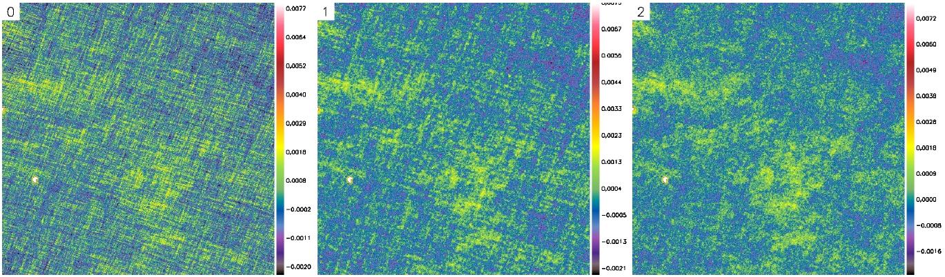
Figure 2: A subfield of the HEVICS survey (Davies et al. 2010), about 2.2 degrees on a side, from 160-micron data processed in three different ways: 0) No drifts (on timescales shorter than the scan leg duration) have been subtracted. 1) The iterations to subtract the individual drifts all have the minimum time step $T_{c}$ . 2) They have successive time steps of $27\times T_{c}$, $9\times T_{c}$, $3\times T_{c}$ and $T_{c}$. The display emphasizes very diffuse structures.

3.6 Detection of other artefacts

3.6.1 Masking of brightness discontinuities

During tests conducted on various PACS datasets, the presence of brightness discontinuities affecting whole array rows (blocks of 16 pixels) or, less frequently, individual bolometers, was noticed. These artefacts are caused by glitches, and also often by electronic instabilities in the multiplexing circuit, that may come and go during the course of an observation. They are currently not corrected for in the pipeline, but they can impact the quality of the maps, leaving bright or dark bands. Since they are high-frequency features followed by a slow decay or a plateau, they can be corrected neither by the deglitching modules nor by the drift subtraction modules. Examples of such artefacts are shown in Fig. 3.

We have therefore developed a module to detect these discontinuities and mask the subsequent frames. This module handles the average series of each 16-pixel block, and then the series of individual bolometers of each block. Spatial information is used jointly with temporal information, making the detections more robust and more sensitive: the series simulated from the current map are subtracted from the observed series. Candidate discontinuities are found whenever the absolute difference between the signal at a given time and the signal three time steps later exceeds a predefined threshold. A candidate is confirmed if it can be unambiguously distinguished from a real brightness variation caused by a compact source or a steep gradient of emission. To this effect, the median brightness and the standard deviation of the series are computed within four time windows, on each side of the potential discontinuity. A diagnostic is made based on these values to rule out compact sources. In addition, to avoid false detections caused by steep gradients (such as present in molecular clouds or edge-on disks), this diagnostic is combined with a thresholding based on the dispersion of the signal in the neighbourhood of each detection. If the candidate is confirmed, subsequent frames of the array row are masked, until the end of the scan leg or until their average brightness gets back to the pre-discontinuity brightness to within the white noise level.

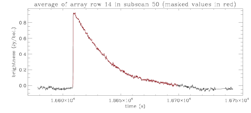
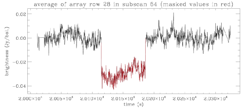
Figure 3: Example of brightness discontinuities in PACS data (left: caused by a glitch; right: caused by an electronic instability). The average series of an array row (16 contiguous pixels) is plotted over a particular scan leg. All the bolometers in the row are affected by the artefact. Overplotted in red are the data that have been masked by the dicontinuity detection module.

3.6.2 Masking of glitches

The software includes the capability to filter glitches remaining after the pipeline processing, whether a deglitching module was run in HIPE or not. They are not interpolated but all affected samples are permanently masked. The detection of glitches shares a portion of its algorithm with modules in charge of computing both the high-frequency noise, and the average and individual brightness drifts. For this reason, the deglitching task is embedded within these modules, and thus split into several steps.

The computation of the high-frequency noise from the spectral densities is made after replacing high-frequency contaminants (both compact sources and glitches) with interpolates (see Sect. 3.3). The samples that are filtered in this process are further examined to separate glitches from real signal. Glitches must simultaneously show a significant deviation from the median signal at their location, and exceed three or four times this reference signal in absolute value (to avoid flagging the sidelobes of a bright compact source). An example of the effectiveness of this approach is shown in Sect. 5.1.2. This is especially useful for SPIRE, because the pipeline includes Fourier-filtering tasks, that can strongly amplify undetected glitches in some instances, as shown in Fig. 15. This problem may be alleviated by using second-level deglitching, or can be dealt with by Scanamorphos.

The computation of the brightness drifts makes use of some simple statistics on bolometer crossings, in order to filter out those with large standard deviations, to protect compact sources (see Sect. 3.5.1). These statistics can also be used to detect glitches. The separation between glitches and real signal with a strong brightness gradient is made by estimating gradients and standard deviations just before and just after the suspect samples. This second deglitching is bypassed when the stability length, determining the pixel size of the grid used for drifts computation, is large compared with the beam FWHM.

3.6.3 Detection of transient sources

Asteroids or other transient sources, that are present at a given location in one scan but have moved or vanished in the other scans, are also detected. The method used to detect them and distinguish them from glitches is based on the fact that they produce a coherent signal for all bolometers as the latter cross the source, while glitches do not. They are dealt with at the same time as glitches in step 7 of Section 3.1. They will thus be ignored if the deglitching is deactivated.

If asteroids are detected, a transient-signal map is produced at the end of the processing, using the same spatial grid as the other final maps. In this map, only the affected portions of the bolometer series are projected, and not those when the bolometers were not illuminated by the asteroids. In this way, it is possible to locate them and to obtain an estimate of their true brightness, whereas they appear dimmer in the nominal signal map (if they are present in one of two scans at a given position, their brightness will be roughly divided by two).

3.7 Projection

At the end of the processing, a final projection produces a sky map, a weight map, an error map and a low-frequency noise map, stored together in a FITS data cube. The low-frequency noise map includes the sum of the drifts subtracted at each step. The signal is weighted by the inverse square white noise of each bolometer. The gnomonic projection is used.

The brightness unit is different for both instruments. The flux calibration of SPIRE is valid for point sources, and voltages are converted to Jy per beam by the pipeline. To obtain extended-source flux calibration, the maps have to be divided by the average beam area. Since the associated uncertainties are larger than those of the point-source flux calibration, and since beam areas may continue to be refined in the future, it is best to apply this correction outside the map-making software. SPIRE maps produced by Scanamorphos are thus in Jy per beam. For PACS, the data are initially in Jy per array pixel, and are converted to Jy per map pixel by Scanamorphos. The default pixel size, approximately one fourth of the FWHM, better samples the point response function (PRF) than that recommended for the projection within the SPIRE pipeline (between 0.33 and 0.4 times the FWHM, depending on the wavelength).

In the SPIRE pipeline, each sample is projected entirely to the closest pixel. Since pixel sizes are a large fraction of the FWHM, this method introduces a bias between the beam center and the projection center. This bias varies as a function of the source position relative to the pixel grid, and is up to $a/\sqrt{2}$, where $a$ is the pixel size. We use instead a projection method akin to the drizzling technique (Fruchter & Hook 2002), where the imprint of each sample on the map is a uniform disk of the same area as the default pixel for the final projection (i.e. ${\rm FWHM}^{2}/16$), and of the same center as the beam. This method does not introduce any bias in the projection center, and reduces the standard deviation of the sky with respect to HIPE maps, by a significant amount (in some configurations, by more than 30% if the low-frequency noise has been perfectly removed). This comes at the expense of a slightly larger PRF: the FWHM is increased by 1.5% (and the area by 3%). Note that the projection affects only the PRF profile, and has no incidence on the beam area to be used to convert units of Jy per beam to units of Jy per pixel.

For PACS, our projection also uses the simplifying assumption of axisymmetric bolometers, whereas the bolometers in reality consist of square pixels (with small distortions). The bolometer imprint is chosen to have a slightly smaller area than the true array pixel, just like in the drizzle projection. It is in principle possible to save the corrected signal series and to perform the final projection within the pipeline for optimum accuracy, but the PRF has not been found to be appreciably modified by our projection.

3.7.1 Weight and error maps

The weight map is defined differently from the coverage map produced by HIPE. It is built by coadding the weights, using the same projection as the sky map, and is normalized by the average of the weights (the average is computed over all the valid bolometers and all the scans). For the nominal data acquired at constant scan speed, the weights are defined as the inverse square white noise values. For turnaround data, acquired at lower or higher scan speed, these weights are decreased so that edges of the map, where both nominal and turnaround data can contribute, are not dominated by low-velocity data.

The error map produced by Scanamorphos is defined as the error on the mean brightness in each pixel. It is built using the (unbiased) weighted variance instead of the simple unweighted variance, since weights are used for the projection of the sky map. It does not include any errors associated with the different processing steps in the pipeline, because these errors are currently not propagated. It should however be useful to estimate the random photometric errors, and to filter glitches that may have escaped detection. Elevated errors will be found both at the location of bright compact sources and in pixels affected by unmasked glitches.

Artefacts that may remain when the redundancy is low can also be spotted by comparing the signal map with the “clean” map in the fifth plane of the cube, that is weighted to exclude noisy scans in each pixel. The latter map is produced in general only when there are two or three scans, and is intended as a diagnostic for the presence of artefacts in the signal map (features that are absent in the ”clean” map). It should not be used for scientific purposes, only as an aid to mask bad data.

3.8 Spatial slicing

For deep observations of wide fields, the software has the ability to slice the data into several partially overlapping fields, in order to minimize memory and computing time usage. This is suitable for observations without very extended bright emission, since it cannot be ensured that extended sources are covered by a single sub-field. For each sub-field, all the available redundancy is used as if it were an entire observation. In the end, the different maps are stitched by matching the brightness levels in the parts of the overlap areas where coverage is nominal.

In the various tests that we conducted, we have not found it necessary to reduce the data volume when the processing was done on a machine with a total memory of 48 Gb, but this functionality was used for some deep observations processed on a machine with a total memory of 8 Gb.

It may sometimes be desirable to do the processing in several spatial blocks, even though the available memory is sufficient to process the entire observation at once. If the observation is long and the subtraction of the short-timescale average drift is required, limitations on the size of the drift differences matrix can make the minimum timescale for the average drift computation longer than that for the individual drifts computation. It is then possible to increase the time resolution of the average drift by decreasing the data volume, which is achieved by slicing the field of view into several blocks.

4 Simulations of PACS observations

We now quantify the effect of the processing with Scanamorphos on the data, using simulations. The instrumental artefacts of PACS are more difficult to remove than those of SPIRE, chiefly because the low-frequency noise has a much greater amplitude with respect to both the signal and the high-frequency noise, and because the stability lengths are greater with respect to the FWHM (Sect. 3.2). Additional complexities arise from the presence of frequent brightness discontinuities (see Sect. 3.6.1), a sampling rate divided by two in parallel mode for the blue array, and a quantization noise that is in general a large fraction of the high-frequency noise (Sect. 3.3). Consequently, our simulations are restricted to the PACS instrument, for which it is more meaningful to demonstrate the response of Scanamorphos.

4.1 Star formation region

Since no artificially-made input will ever capture the true complexity of the sky, we simulated an input sky using a map produced from real observations of a Galactic star formation region, NGC 6334, studied by Russeil et al. (2012). These observations were made in parallel mode for a duration of 7.29 hours, at the scan speed of 20 arcsec/s, and we used the blue band (70 $\mu$m) for the simulation. The total field area is a little over 3 square degrees. The redundancy is limited to the minimum recommended, since the observation is made of two scans.

The noise series are space calibration measurements taken during a staring observation, and shall be used by the PACS simulator (Hervé Aussel, private communication). They are affected by glitches and very frequent brightness discontinuities. This staring observation was not long enough to cover the duration of the simulation. Therefore, we used all the data from the blue array, in both the 70 and 100 $\mu$m bands successively, for a total duration of 5.91 hours. There is a slight bias in the average white noise levels of both datasets, due to the change of filter, but only at the $0.6\sigma$ level (3.5% of the absolute white noise values), so we do not correct for it.

To circumvent the fact that the duration of the noise observation still falls short, we extrapolated the noise series in the following way: for each bolometer in turn, we randomly select chunks of 100 s in the observed series (excluding the start affected by strong transients from the calibration sources systematically observed before each science observation), and concatenate them to the signal after matching their initial brightness with the final brightness of the preceding chunk. The original time indices of the chunks are different for all bolometers, so that the average noise cannot repeat itself. In addition to the five unstable rows that are automatically excluded for Galactic fields (Sect. 2.3 and Fig. 3b), we detected a total of 132 brightness discontinuities affecting whole array rows, and 80 jumps affecting single bolometers, but they were not corrected (since this was impossible when using the /galactic option at the time the simulation was made and analyzed). Figure 4 shows the average series of the noise, to demonstrate that the simulation contains both a mild thermal drift and uncorrelated noise.

Figure 4: Average over all valid bolometers of the noise series introduced in the simulation (in Jy per bolometer). The second scan is plotted with an offset for clarity. The dashed lines indicate, for each scan, the time after which the series had to be extrapolated (see the text).

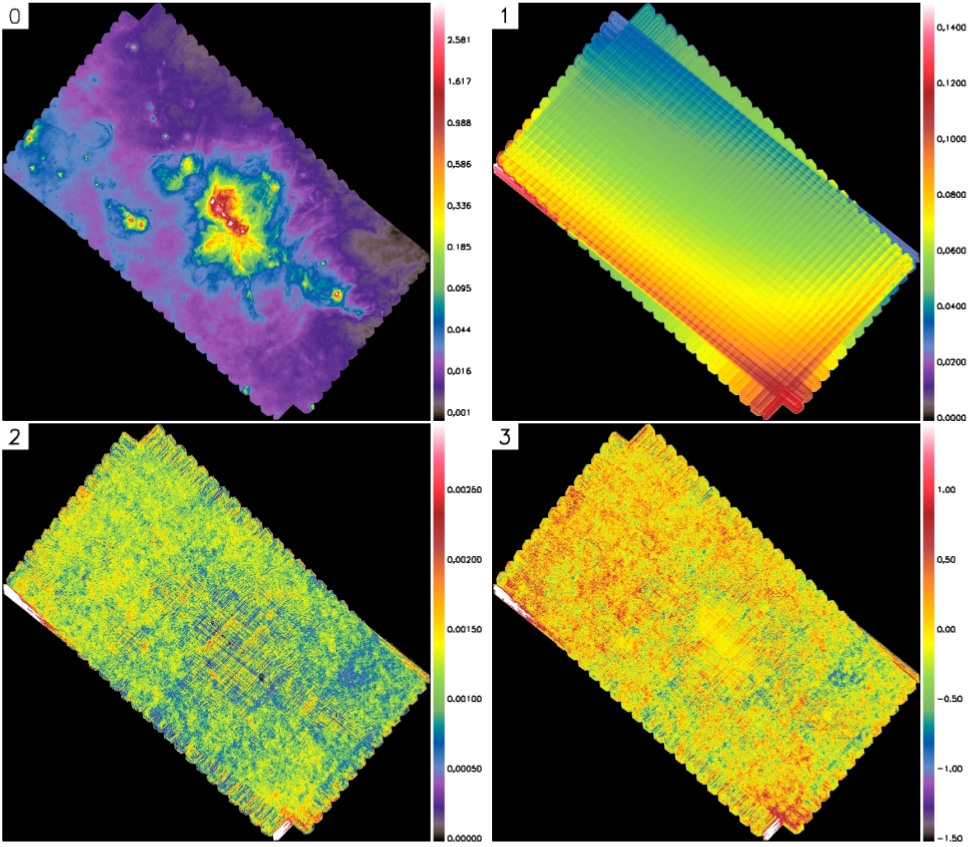
Figure 5: Simulation of the star formation region NGC 6334. 0) Ideal map (with an applied brightness cut of 4 Jy/pixel; the maximum brightness is 33.6 Jy/pixel). 1) Map of the noise added to the input sky, with the flux calibration offsets removed. The displayed brightness range is 0 to 0.15 Jy/pixel. 2) Difference of the processed map and the ideal map (range 0 to 3 mJy/pixel). 3) Same difference map, with the median offset removed, and normalized by the error map produced by Scanamorphos (range $-1.5\sigma$ to $+1.5\sigma$).

We simulated time series from the map of NGC 6334, added the noise series to them, and then applied to the result the same digitization as that affecting the staring observation (i.e. the quantized values of the result have the same minimum and the same digitization step). In these data, the digitization noise represents 50% of the white noise on average. This simulation was processed with the /galactic option and the default choices (deglitching, subtraction of the average drift, inclusion of turnaround data, projection on pixels of the default size). We checked that disabling the short-timescale average drift subtraction produces virtually identical results. We also projected on the same astrometric grid two other maps: that of the noise from the staring observation, after subtracting the flux calibration offsets to obtain the same median brightness for all bolometers; and that of the idealized input signal from the map of NGC 6334, after eliminating the five unstable rows that are always excluded for Galactic fields, and without any quantization nor weighting of the signal. We will refer to these three maps as the processed map, the noise map and the ideal map, respectively.

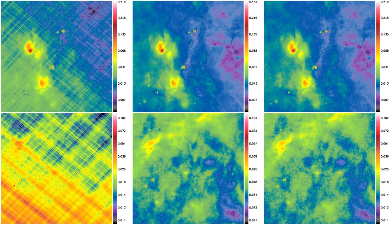
Figure 6: Two small portions of the total field of view of the simulation of NGC 6334, $14^{\prime}$ on a side, are shown (in Jy/pixel). From left to right: (ideal + noise) map, displayed with a brightness offset; ideal map; processed map, displayed with the general offset of 1.1 mJy/pixel. The flux calibration offsets have been removed from the noise map, as above.

Figure 7: Left: The deviation from the flux measured in the ideal map, in units of the photometric uncertainty $\sigma$, is plotted as a function of this flux. The deviation introduced by the noise map (the initial error) is plotted in blue, and the deviation in the processed map (the residual error) in black. The yellow diamonds are averages computed in bins of 0.2 dex for the initial error, and the red diamonds represent the same for the residual error. To guide the eye, horizontal lines at $\pm 3\sigma$ and zero are overplotted. Right: The residual error is plotted as a fonction of the initial error, both in units of $\sigma$ (notice the different scale for both axes). Sources above $5\sigma$ are in black, and sources above $15\sigma$ in red. The grey lines show the $\pm 3\sigma$ limits, and the horizontal lines in the middle show the average residual error.

Figure 8: The photometric uncertainty $\sigma$ (measured in the processed map) is plotted as a function of the uncertainty $\sigma\prime_{\rm initial}$ measured in the noisy map (sum of the ideal and noise maps). Both are normalized by the true flux $F_{70}$. The shift from the dashed line indicates by how much the noise has been reduced in the map. The red diamonds indicate the average values in the same flux bins as in Figure 7 (left), and their size increases proportionally with $\log F_{70}$. For high fluxes, the photometric uncertainty is completely dominated by the binning noise that is present in the ideal map; it results from projecting in finite pixels a signal that has a very steep spatial gradient, i.e. a bright compact source.

We analyze the results in several ways. First, we display the difference between the processed map and the ideal map, to assess the effect of the noise and processing on the very extended emission (Fig. 5). There is a slight offset between the processed and ideal maps (of 1.1 mJy/pixel), but offsets are of no relevance since Herschel instruments are not absolute photometers. The zero-level of the sky emission can only be calibrated with other instruments. Thus, we consider that the subtraction of this global offset is not a necessary or even meaningful task for Herschel mapping tools. What is important to notice is that there is no significant brightness gradient in the difference map, hence that the average drift was satisfactorily removed. The imprint of the sources is also not discernible, which implies that the extended emission was preserved throughout the field. Low-level structure due to imperfect drift subtraction is present, but remains within the photometric errors. Figure 6 shows details of the three maps in two small portions of the field, chosen among the regions of relatively diffuse emission.

Then, we perform simple aperture photometry on all the compact sources (point sources or slightly extended sources such as background galaxies) that we can find in the ideal map wherever the coverage is nominal, and apply the same apertures to the three maps. Although many sources sit on a very structured local background, we make no attempt to correct for contamination from nearby sources or underlying extended emission, since our aim is not to measure the absolute fluxes, but to test the flux conservation. We use an aperture of 10 pixels in diameter, i.e. $14\arcsec$ or 2.5 FWHM, and an annulus for the local background of inner diameter 10 pixels and outer diameter 24 pixels, i.e. $33.6\arcsec$ or 6 FWHM. We measure photometric uncertainties, noted $\sigma$, by adding in quadrature the error on the mean brightness in each pixel (from the error map produced by Scanamorphos). They are measured in the processed map to obtain realistic values, and not in the ideal map, since by construction the latter does not contain any white noise. If the drifts had been perfectly removed, $\sigma$ would be dominated by the white noise, but since residual errors are correlated because of the small pixel size, these uncertainties are underestimated. We obtain 879 compact sources detected in the ideal map at the $5\sigma$ level or more.

With these measurements, we test two properties at small spatial scales: whether flux is conserved, and to which extent the noise is reduced. Figure 7 shows that the photometric errors initially introduced by the drifts, up to $20\sigma$, are greatly reduced by the processing, the residual errors being all within $3\sigma$. There is a slight residual average bias for faint sources (below 170 mJy), but well within the photometric error bars, of the order of $-0.5\sigma$. This bias disappears when the detection significance level increases, and would probably also disappear for faint sources by increasing the redundancy in the observations, i.e. increasing the number of scans or observing in nominal mode. Figure 8 shows in addition by which amount the photometric uncertainty computed from the error map is reduced, as a function of the initial uncertainty and of the source flux. We conclude that Scanamorphos is both flux-conserving and efficient at reducing the noise, including on small spatial scales.

4.2 Nearby galaxy

We now simulate a field with a much smaller dynamic range, typical of extragalactic observations. To generate the input sky, we use an ancillary Spitzer observation at 8 $\mu$m of the face-on galaxy NGC 3184, included in the SINGS and KINGFISH samples (Kennicutt et al. 2003, 2011). Since this map (showing mostly the emission from polycyclic aromatic hydrocarbons in this band) contains both compact and very diffuse emission, it provides a realistic test case for the far-infrared emission of galaxies.

We first subtract a tilted plane to rectify the background, then convolve the map to the resolution of PACS at 160 $\mu$m, using the kernel and tool provided by Aniano et al. (2011), and rescale the peak brightness (of the nuclear regions) to that of NGC 3184 at 160 $\mu$m.

The noise series are extracted, like those of the previous simulation, from a staring observation (courtesy Marc Sauvage and PACS Instrument Control Center). They contain glitches but only a very shallow thermal drift. Since their quantization step (Sect. 3.3) is twice that of the extragalactic observations, we have to correct for this before adding the noise series to the simulated sky series. Otherwise, the sensitivity would be artificially decreased with respect to real observations. We thus average the noise series from two successive observations to divide the quantization step by two, and add back to the result $\sqrt{0.5}$ times the initial white noise. The (sky + noise) series were then digitized to match the quantization step of the noise, as in Section 4.1. The resultant digitization noise to white noise ratio is of the order of 30%, the same as in the real 160 $\mu$m observation of NGC 3184.

This simulation was processed with the /jumps_pacs option and the default choices. In addition to the maps described for the previous simulation, we also produce an (ideal + white noise) map, where only white noise has been added to the simulated sky series, and the result digitized, to illustrate the erosion of the sensitivity that results from this irreducible noise component. This map is not used for the analysis: the brightnesses of the simulation are compared with those of the ideal map (without any noise nor quantization). The results from the normal processing are also compared with those obtained when the drifts are subtracted only on long timescales (i.e. the processing is stopped after the baseline subtraction). The corresponding map is called the noisy map or the deglitched noisy map, depending on whether the first iteration of the deglitching after baseline subtraction was performed or not.

Figure 9 shows the various signal and error maps, and Figure 10 the azimuthally-averaged surface brightness profiles. The photometric uncertainties are reduced by the subtraction of the short-timescale drifts, and the errors (the difference between the processed map and the ideal map) are everywhere below the photometric uncertainties, as estimated from the error map produced by Scanamorphos (Fig. 9). Some residual artefacts are visible at the location of the galaxy, but their amplitude remains mostly below the $2\sigma$ significance level. As demonstrated by Figure 10, the processing brings significant improvements in the recovery of diffuse emission, at radii beyond about 150^′′.

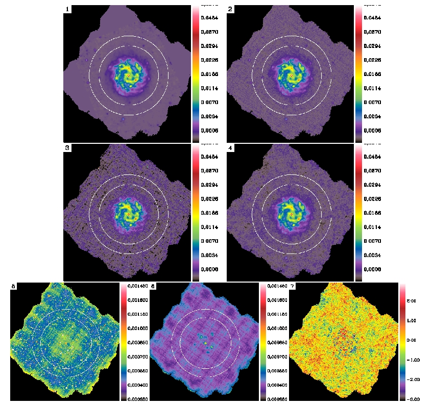
Figure 9: Maps of the galaxy simulation (in Jy/pixel). 1) Ideal map. 2) (Ideal + white noise) map (see text). 3) Noisy map, with only long-timescale drifts (baselines) subtracted. 4) Processed map. 5) Error map associated with the noisy map. 6) Error map associated with the processed map, displayed with the same brightness scale. 7) Difference between the processed and ideal maps, normalized by the error map produced by Scanamorphos (range $-3\sigma$ to $+3\sigma$). The white circles show the galaxy and background apertures.

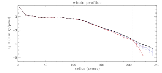
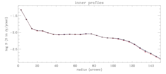
Figure 10: Surface brightness profiles obtained from the ideal map (in black), the deglitched noisy map (in red) and the processed map (in blue). Each annulus has a width of 2 pixels, i.e. ${\rm FWHM}/2$ . The vertical dashed lines in the first panel indicate the $R_{25}$ minor and major axis radii in the B band.

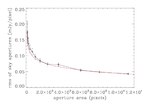
Figure 11: Standard deviation of the average sky brightness in independent apertures of equal area, as a function of aperture area. The vertical bars represent the typical pixel-to-pixel standard deviations within individual apertures. The function shown in red was used to extrapolate the results to larger apertures, since the map is too small to define several background apertures of the same size as the galaxy. The dashed line represents the same quantity for a simulated pure Gaussian noise, normalized to the smallest aperture area, showing that the measurements are dominated by correlated errors.

We also measure the global flux of the galaxy within a radius of 90 pixels, and the background within an annulus of inner and outer radii of 90 and 120 pixels, i.e. $256.5^{\prime\prime}$ and $342^{\prime\prime}$ (as indicated in Fig. 9). To estimate a background uncertainty that takes into account the correlation of errors in adjacent pixels, and in larger areas due to long-timescale drift residuals, we use measurements of the average sky brightness in several sets of independent apertures. For each set, an annulus around the galaxy is divided into equal-area angular sectors, defining our sky apertures. From one set to the next, the widths of the annulus and angular sectors are progressively increased. Fig. 11 shows the standard deviation of the independent sky measurements as a function of aperture area. The extrapolation of these results to the area of integration of the galaxy flux gives us an estimate of the component of the background uncertainty that has to be summed linearly. We define the total uncertainty as $\Sigma_{\rm tot}=\sqrt{N^{2}~{}\sigma_{\rm b~{}corr}^{2}+N~{}\sigma_{\rm b~{}rand}^{2}+\Sigma_{\rm phot}^{2}}$ where N is the number of pixels of the galaxy aperture, $\sigma_{\rm b~{}corr}$ is the correlated uncertainty on the background just discussed, $\sigma_{\rm b~{}rand}$ is the random uncertainty on the background (obtained from the pixel-to-pixel standard deviation of the sky brightness within the background annulus), and $\Sigma_{\rm phot}$ is the photometric uncertainty from the quadratically-summed error map. The error budget is completely dominated by the $N~{}\sigma_{\rm b~{}corr}$ term for this dataset (by 99%). With 1-$\Sigma_{\rm tot}$ error bars, we obtain a total galaxy flux of ($58.81\pm 0.05$) Jy in the ideal map, ($56.31\pm 0.70$) Jy in the deglitched noisy map, and ($58.06\pm 0.69$) Jy in the processed map. The uncertainty increases from 0.7 Jy to 1.1 Jy if $\sigma_{\rm b~{}corr}$ is not extrapolated but assumed constant for aperture areas greater than our last measurements in Fig. 11. In this simulation, the global flux is thus recovered within 1.2 to $0.8~{}\Sigma_{\rm tot}$ (1.4% of the true flux) in the processed map, while it is 3.7 to $2.4~{}\Sigma_{\rm tot}$ below the true flux (4.4% of the true flux) in the noisy map.

5 Examples and visualization step by step

We apply below the algorithm to diverse datasets (with different types of structures and brightnesses, in parallel-mode or nominal observations, with various scan speeds), taken during the Science Demonstration Phase. We provide visualizations in terms of time series and maps at each important step of the processing. We illustrate different details on each dataset. All the maps displayed below are in units of Jy per beam for SPIRE and Jy per array pixel for PACS, except the final maps for PACS whose brightness unit is Jy per map pixel. Only the final maps are displayed in the standard astronomical orientation (north to the top and east to the left). Each dataset is identified by its observation day (OD) and observation block numbers (obsid).

Table 1 summarizes the field sizes, processing options, drifts amplitudes and indicative processing times (excluding the time needed for the initial data ingestion and reformatting) for all observations presented here as examples, and a few others in addition. The code has been reasonably optimized for speed, but gains shall still be possible. The processing was made on a Linux machine with a CPU frequency of 2.93 GHz and a total memory of 48 Gb; but it is possible to process most datasets, not extremely deep, with much less memory. Multithreading, used by default by IDL on multiprocessors, had to be deactivated on this particular machine to improve performance (processing times decreased by 20 to 35% on the few tested datasets). In this configuration, the ratio of the processing time to the observation duration is of the order of 7% at 250 $\mu$m, 5% at 350 $\mu$m, and 2% at 500 $\mu$m for relatively short observations ($<10$ hours) made with the SPIRE arrays; 25%, 15%, and 7% at 250, 350, and 500 $\mu$m, respectively, for the very deep GOODS-N observations; for the PACS arrays, that are made of a much larger number of bolometers, this ratio ranges from 50 to 75% at 70 $\mu$m and 15 to 20% at 160 $\mu$m, in the cases presented in Table 1. For large data volumes, the longest tasks are the baseline subtraction and average drift subtraction. The individual drifts subtraction is comparatively very fast. Note that we have adopted the shortest possible timescales for the drifts, and that the processing times may be decreased by enlarging the timescale for the average drift.

Table 1: Processing parameters for a few test observations

field	size	options	Ns	tobs	tproc	Tc	Niter		ampD / HF		ampD (Jy/bol.)
				(s)	(s)	(s)	aver.	indiv.	aver.	indiv.	aver.	indiv.
SPIRE
NGC 6822 250 $\mu$m	$20^{\prime}\times 20^{\prime}$	none	6	2453	182	0.59	1	2	141.	2.2	4.221	0.066
NGC 6822 350 $\mu$m					112	0.81	1	2	149.	2.0	4.819	0.065
NGC 6822 500 $\mu$m					54	1.18	1	2	169.	2.4	6.905	0.096
NGC 6946 250 $\mu$m	$30^{\prime}\times 30^{\prime}$	none	4	2430	178	0.43	1	2	52.	1.6	1.591	0.048
NGC 6946 350 $\mu$m					126	0.43	1	2	57.	1.5	1.860	0.050
NGC 6946 500 $\mu$m					59	0.59	1	2	67.	1.6	2.762	0.065
Rosette 250 $\mu$m	$88^{\prime}\times 69^{\prime}$	/parallel,	2	19317	1245	0.9	1	2	242.	11.	6.109	0.285
Rosette 350 $\mu$m		/galactic			790	1.3	1	2	255.	11.	6.890	0.294
Rosette 500 $\mu$m					384	1.8	1	2	280.	17.	9.646	0.598
Atlas 250 $\mu$m	$245^{\prime}\times 224^{\prime}$	/parallel	2	55209	10056	0.6	2	2	1332.	58.	33.11	1.442
Atlas 350 $\mu$m					8110	0.6	2	2	1457.	55.	38.70	1.456
Atlas 500 $\mu$m					6791	0.6	2	2	1704.	73.	57.73	2.460
GOODS-N 250 $\mu$m	$33^{\prime}\times 33^{\prime}$	none	60	47696	12135	0.59	2	2	743.	2.0	22.50	0.061
GOODS-N 350 $\mu$m					7200	0.81	2	2	812.	1.9	25.70	0.060
GOODS-N 500 $\mu$m					3354	1.18	2	2	976.	2.1	42.06	0.090
PACS
NGC 4559 70 $\mu$m	$15^{\prime}\times 15^{\prime}$	/jumps_pacs	12	6838	4878	0.7	1	3+3	131.	9.2	1.514	0.107
NGC 4559 100 $\mu$m			12	6838	4934	0.7	1	3+3	90.	8.4	1.027	0.095
NGC 4559 160 $\mu$m			24	13676	2650	0.9	1	3+3	95.	11.	2.034	0.229
Centaurus A 70 $\mu$m	$36^{\prime}\times 36^{\prime}$	none	8	16633	12635	0.7	1	3+3	28.	9.0	0.314	0.100
Centaurus A 160 $\mu$m			8	16638	3094	0.9	1	3+4	8.4	11.	0.175	0.230
M 81 70 $\mu$m	$40^{\prime}\times 40^{\prime}$	/jumps_pacs	8	22190	16199	0.7	1	3+3	24.	8.6	0.315	0.112
M 81 160 $\mu$m			8	22190	3886	0.9	1	3+4	13.	11.	0.387	0.320
Rosette 70 $\mu$m	$91^{\prime}\times 72^{\prime}$	/parallel,	2	19887	9814	1.2	1	3+4	102.	38.	1.165	0.436
		/galactic

Note. — The table entries are: name and wavelength; area with nominal coverage; options on the command line; number of scans $N_{\rm s}$; observation duration; indicative processing time; minimum timescale T_c of the drifts; number of iterations for average and individual drifts, respectively (for PACS, the first 3 iterations for individual drifts are made with a time resolution of 27, 9 and 3 times T_c, and the following of T_c); amplitude of the total drifts (including baselines) in units of high-frequency noise, for average and individual drifts, respectively; amplitude of the total drifts in Jy per bolometer, also for average and individual drifts, respectively.

5.1 Application to SPIRE data

5.1.1 Rosette nebula (OD 159, obsid 1342186121 and 1342186122)

The Rosette nebula was observed during the Science Demonstration Phase (Motte et al. 2010, and references therein) with two scans in parallel mode, at low scan speed ($20\arcsec/{\rm s}$). Illustrations for the 250 $\mu$m band are provided in Figure 12.

On this dataset, we show the subtraction of baselines, i.e. long-timescale drifts, when the /galactic option is used. The amplitude of the short-timescale drifts is so small, compared with the signal brightness, that their removal is not directly discernible in the maps. Notice how simple baselines are only a first step in the subtraction of large-scale drifts, and are insufficient to eliminate the striping caused by these drifts. The module computing residual baselines from the redundancy is needed to completely subtract large-scale drifts.

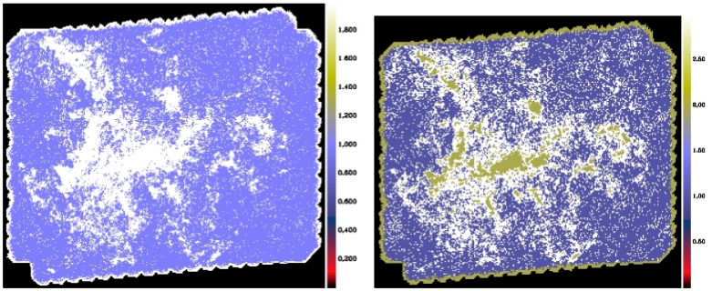
Figure 13: Drift mode grids for the Rosette observation at 250 $\mu$m (left) and 350 $\mu$m (right). Whenever possible, the drift computation modules switch to a finer spatial grid when they encounter coarse pixels within which the dispersion of the signal is higher than a predefined threshold. At 250 $\mu$m, the number of samples per stability length is too small to be able to switch to a finer grid, whereas it is sufficient at 350 $\mu$m (for which the fine grid is coded by the value 3, in white).

Figure 13 illustrates, on the same dataset, how the drift subtraction modules automatically detect non-uniformities within the chosen stability length, and reject the corresponding samples to avoid a contamination of the drifts by sources and glitches (see Sect. 3.5.1). The left image shows at 250 $\mu$m, for each pixel of size equal to the stability length of the drifts, whether the drift computation was enabled (in blue) or not (in white). The right image shows the same thing at 350 $\mu$m, where the stability length becomes large enough to switch to a finer grid (with pixels half as wide) if necessary: it shows whether the drift computation was enabled on the original grid (in blue), enabled only on the finer grid (in white), or impossible (in yellow). Such maps (displayed in visualization mode) delineate very well the location of compact sources and steep brightness gradients.

5.1.2 Atlas field (OD 192, obsid 1342187170 and 1342187171)

This low-brightness field, containing both very diffuse Galactic emission and distant galaxies, was observed with two scans in parallel mode, at high scan speed ($60\arcsec/{\rm s}$). The survey from which this observation was extracted is described by Eales et al. (2010).

On this dataset, we particularly illustrate the subtraction of the average drift, compared with the temperature drift correction implemented in the pipeline, and the masking of residual glitches amplified by Fourier filtering employed in some pipeline modules. Each effect is illustrated in the array where it is the most prominent, PMW (350 $\mu$m) for the average drift and PSW (250 $\mu$m) for glitches. The stability length was increased to 2 and 1.5 times the FWHM for PSW and PMW, respectively.

Two features are remarkable in the map of detected glitches (Fig. 14). It contains long trails corresponding to glitches not detected within the pipeline and then amplified by the electrical filter response and the bolometer time response corrections; and the imprint of the whole array is visible in many places, corresponding to glitches that simultaneously affect the whole array. This type of glitches is frequently seen in SPIRE (Griffin et al. 2010; Swinyard et al. 2010). Figure 15 shows a striking example of the glitch amplification effect, on a portion of the signal of a PSW bolometer, before and after the glitch masking module of Scanamorphos has been run (Sect. 3.6.2).

Figures 16 and 17 illustrate the subtraction of the average drift, which is particularly challenging for this field, because its time derivative varies abruptly during the first scan, and does not conform to the thermal noise model implemented in the pipeline; in addition, the redundancy is minimal, with only two scans acquired at high scan speed and with the lowest sampling rate. The subtraction of baselines removes the linear component of the drift, but leaves strong residuals, that are essentially confined to the first scan. The comparison between the two scans mapped separately emphasizes these residuals. Figure 17 shows that after the drift subtraction, the two scans agree almost perfectly in the region where they overlap (i.e. with no sign of residual average noise, only differences caused by the white noise and pointing errors). Note that the only residuals from the temperature drift are found on the edges of the map that are covered by only one scan, i.e. outside the field of view with nominal coverage. For optimum results, when the thermal drift varies so abruptly, it is also possible to perform the average drift subtraction within Scanamorphos after the thermal drift has been attenuated by the relevant pipeline module.

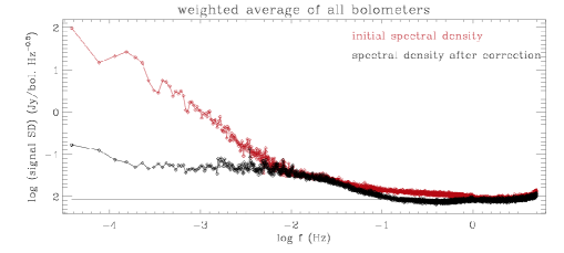
Figure 18: Spectral densities computed from the Atlas 350 $\mu$m observation. Top: Spectral density of the signal, computed on the length of a scan (weighted average of the spectral densities of all valid bolometers), after the processing (in black), compared to the initial spectral density (in red). Bottom: Spectral densities of the subtracted average drift (left), and of the individual drifts (right), computed on the length of a scan and on the coarse time grid (hence the different frequency scale). They are simple averages of the spectral densities of all valid bolometers. In each panel, the horizontal lines represent the spectral density of the high-frequency noise. The dashed lines are 25% and 75% quartiles. Before computing the Fourier transform, the longest baselines were removed from the time series, and the rectified time series were apodized with a $\sin^{2}$ function at both ends, on each scan separately.

Spectral densities of the initial signal, of the signal corrected for drifts, and of the drifts themselves are shown in Figure 18. The spectral index of the drift spectral density is close to $-1$ .

5.1.3 NGC 6822 (OD 145, obsid 1342185533)

This dwarf galaxy, containing both compact HII complexes and diffuse emission, is located behind relatively bright cirrus filaments. It was observed with 6 scans at the nominal scan speed of 30 arcsec/s (Galametz et al. 2010).

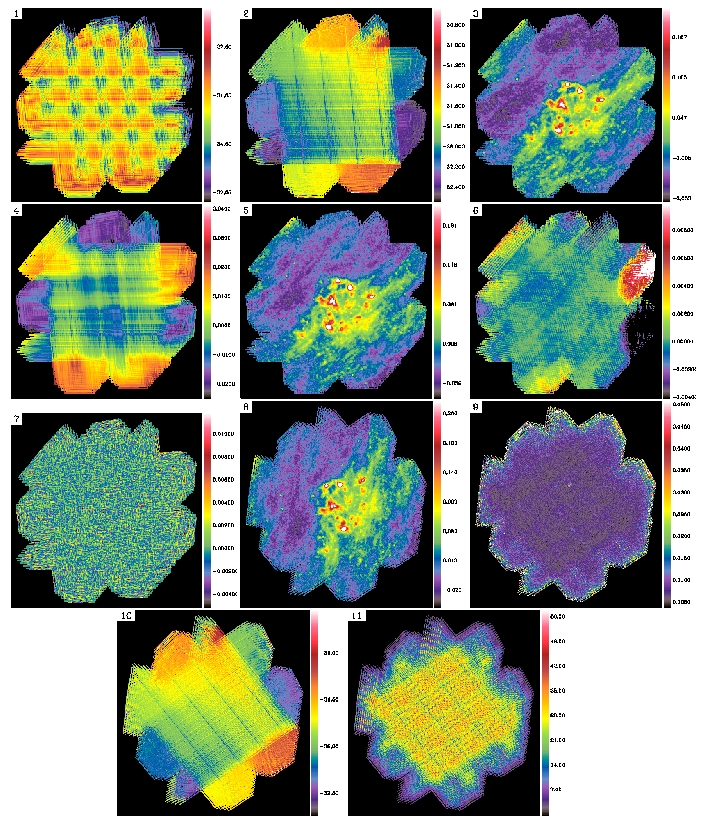
Figure 19: Successive steps of the processing of the NGC 6822 250 $\mu$m observations illustrated by maps, showing the following: 1) raw level-1 data; 2) simple baselines obtained by linear fits; 3) data after subtraction of the simple baselines; 4) residual baselines derived from the redundancy; 5) data after subtraction of the residual baselines; 6) average drift subtracted at the first iteration (and glitches masked); 7) individual drifts subtracted at the second iteration; 8) final map; 9) error map; 10) total drifts (dominated by baselines); 11) weight map. Maps 1, 2, 4, 6 and 7 are projected on a coarse spatial grid, and the other maps are projected on a fine grid (with pixels of FWHM/4 on a side). Note that the very faint filamentary structures superposed on the westernmost part of NGC 6822 (to the right) are not caused by residual drifts: they are not aligned with any of the two scanning directions, but with the general direction of the cirrus filaments.

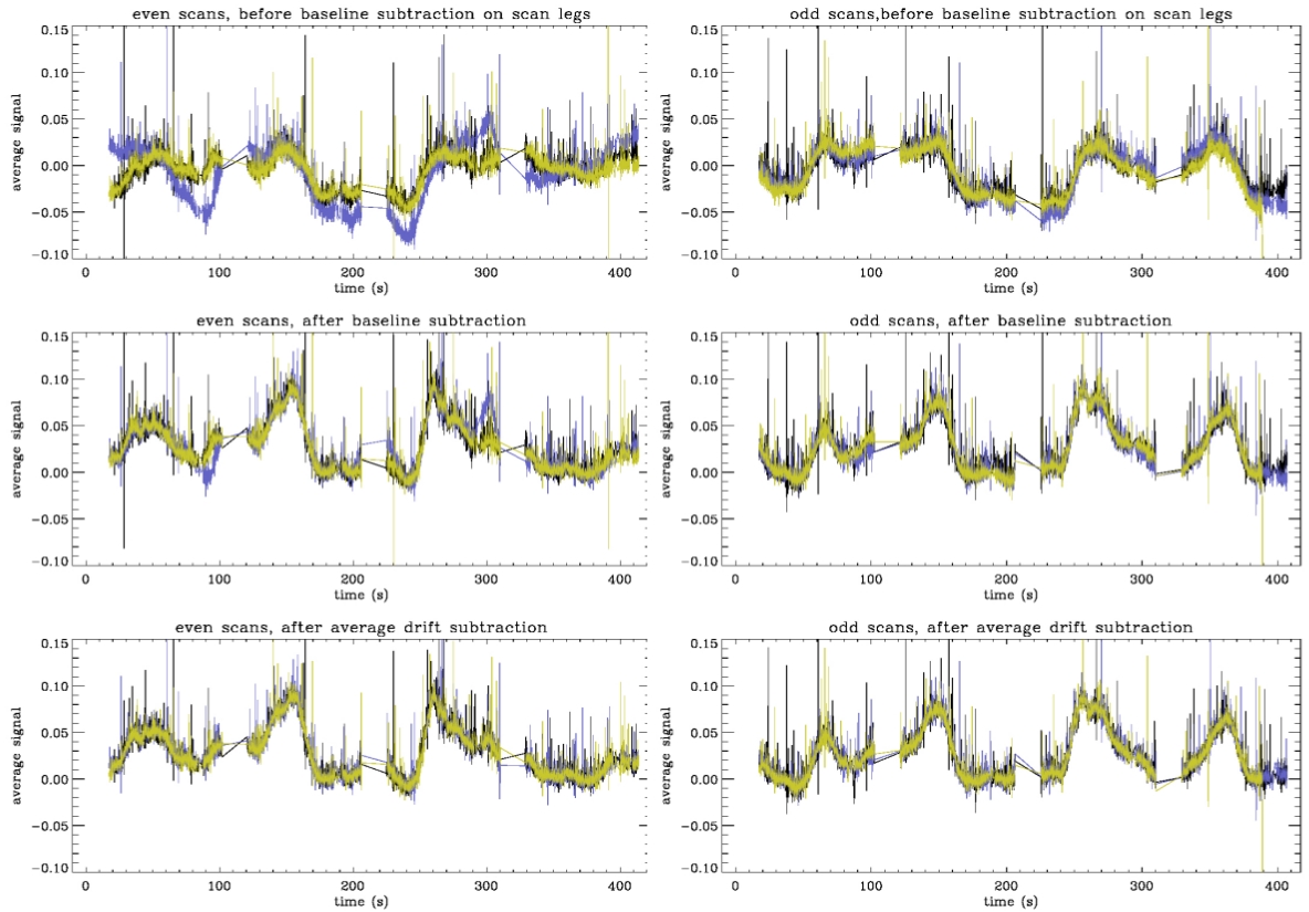
Figure 20: Another way of looking at the average drift subtraction, in the time domain (from the NGC 6822 250 $\mu$m observation). Average signal of even-number scans (left; in the same scanning direction) and odd-number scans (right; in the orthogonal direction), in units of Jy/beam, before the baseline subtraction performed on scan legs (top), after full baseline subtraction (middle), and after subtraction of the average drift (bottom). Different scans coded by different colors are superposed after applying a time shift, such that a given time corresponds approximately to the same spatial coordinates. After the baseline subtraction, there are still significant differences between successive scans (mostly in the even-scan direction, at times close to 90 s and 300 s) that vanish after applying the average drift subtraction.

This example shows how baselines and drifts (both the average and individual components) can be robustly derived even in the presence of complex structures on the largest scales of the map (such as cirrus emission here), when the /galactic option is not used. Figure 19 also shows that the raw data and total drifts are completely dominated by the linear baselines. Figure 20 demonstrates in addition that it is possible to separate the residual non-linear average drift from the complex sky signal, by the method implemented in Scanamorphos.

5.1.4 NGC 6946 (OD 116, obsid 1342183366)

This large spiral galaxy was mapped with 4 scans at high scan speed (60 arcsec/s) during the Performance Verification phase, and is part of the KINGFISH program (Kennicutt et al. 2011).

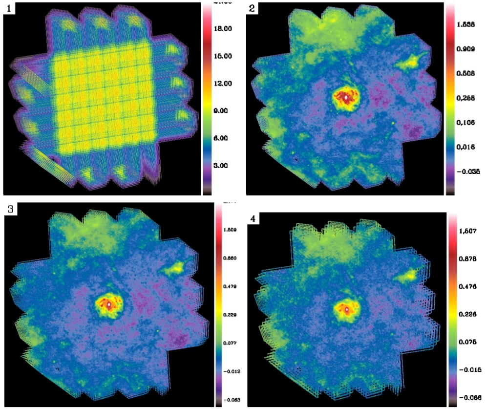
Figure 21: Final maps obtained after processing the NGC 6946 observations: 1) weight map at 250 $\mu$m, showing the large turnaround regions with sparser coverage, due to the high scan speed; 2, 3, and 4) final maps at 250 $\mu$m, 350 $\mu$m, and 500 $\mu$m, respectively.

The stability length was automatically increased to 1.5 times the FWHM for PSW. Since the average drift is very close to being purely linear for this particular observation, making it easy to subtract with simple baselines, we do not show the intermediate results, but only the final maps (Fig. 21). Even though wide parts of the map have non-nominal coverage, due to the high scan speed and thus the longer deceleration distance between successive scan legs, it is possible to accurately recover the sky structure in these edges, as shown by the maps, as long as they are covered by two scans (in the same scanning direction).

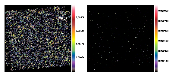
Figure 14: Maps of glitches (in absolute value) detected and masked within the high-frequency noise computation module (left) and subsequently within the average drift subtraction module (right). The dataset is that of the Atlas field, in the PSW array. The first map shows examples of amplified glitches leaving long trails, and glitches occuring simultaneously in many bolometers of the array. The second deglitching (second map) detects only residual glitches that do not exhibit these effects.

Figure 15: Initial signal of a PSW bolometer, containing glitches amplified by some pipeline modules (left), and signal of the same bolometer after running step 5 of the Scanamorphos algorithm, as outlined in Sect. 3.1 (right). Notice that the ordinate range is not the same in both plots.

Figure 16: Average signal of the Atlas 350 $\mu$m observation, before baseline subtraction, when the pipeline processing did not include the temperature drift correction (left), and when it did include the temperature drift correction (right). In this particular (but by no means isolated) case, the SPIRE thermistors fail to provide an acceptable model for the thermal drift. The vertical yellow line shows the limit between the two scans.

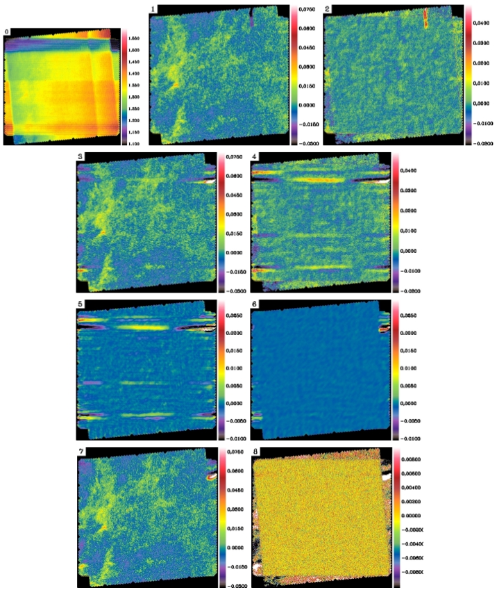
Figure 17: Maps drawn from the Atlas 350 $\mu$m observations to illustrate the impact of the thermal drift and its subtraction by Scanamorphos: 0) data with the pipeline temperature drift correction applied, after simple flux calibration offsets have been removed (the map should be similar to the final map shown in 7 if the pipeline temperature drift correction were of good quality); 1) data with the pipeline temperature drift correction applied, after full baseline subtraction as implemented in Scanamorphos; 2) same, but mapping the difference between the two scans; 3), 4) same as maps 1 and 2, but for data processed without the pipeline temperature drift correction. The results shown in the following maps were obtained from data processed without the pipeline temperature drift correction. 5), 6) maps of the average drift subtracted during the first two iterations; 7) data after subtraction of the drifts; 8) same, but mapping the difference between the two scans. Maps 0 and 2 immediately show the impact of the thermal drift left by the pipeline. Map 8 shows that the empirical drift subtraction carried out by Scanamorphos worked perfectly, except on the edges with non-nominal coverage (only one scan). Notice the different brightness ranges of maps 2-4 and 8.

5.2 Application to PACS data

5.2.1 NGC 4559 (OD 188, obsid 1342187067, 1342187068, 1342187069 and 1342187070)

This spiral galaxy was observed as part of the KINGFISH program (Kennicutt et al. 2011) at nominal scan speed ($20\arcsec/{\rm s}$). The observations were split into four distinct obsid. The blue (70 $\mu$m) and red (160 $\mu$m) filters were used simultaneously during the first and third obsid, and the green (100 $\mu$m) and red filters during the second and fourth obsid. The blue and green maps are each made of 12 scans, and the red map of 24 scans.

One word of caution: since observations in the blue and green filters use the same PACS array, commonly referred to as the blue array, some confusion might arise between the two. When formatting the HIPE data for input to Scanamorphos, one should always check that the selected filter is correct. The module allows this by printing the name of the filter and issuing an error message if necessary.

The scans almost always need reordering before input to Scanamorphos, in such a way that the scanning directions are alternating from one scan to the next. The reason is that this is the default ordering for SPIRE, and that the baseline subtraction module always assumes this order. This is explained in detail in the examples directory of the Scanamorphos distribution. The /vis_traject option allows one to visualize the scan pattern and to check that scanning directions are alternating correctly. In addition, all the scans of a given obsid must have been used before turning to the next obsid made with the same scanning direction.

The stability length was increased to 2.5, 2, and 1.5 times the FWHM at 70 $\mu$m, 100 $\mu$m, and 160 $\mu$m, respectively. Intermediate results of the drifts subtraction for the 160 $\mu$m array can be seen in Figure 22. For these illustrations, the intermediate maps were reprojected on the final pixel grid (instead of the mapping grid used for the processing) in order to make the effect of the low-frequency noise easier to see in the maps. The maps of the drifts were not reprojected, and are thus shown on a coarser grid (with pixels of $3/4$ FWHM on a side).

5.2.2 Rosette (OD 159, obsid 1342186121 and 1342186122)

These observations are the PACS component of the parallel-mode observations already described in Section 5.1.1. We processed only the 70 $\mu$m data. In this example, the high-frequency noise is completely dominated by the quantization noise (Sect. 3.3). The stability length was increased to 4.5 times the FWHM. Notwithstanding the low redundancy, we used a final pixel size of FWHM/4.

Despite the unfavorable observing parameters (high quantization noise and low sampling rate of 5 Hz), Figure 23 shows that the different processing steps perform as expected, and that the final map quality is very good, compared with maps produced within the pipeline (not shown here). Scanamorphos preserves both diffuse emission and compact sources, whereas the use of polynomial baselines or Fourier filtering in the pipeline strongly distorts extended emission.

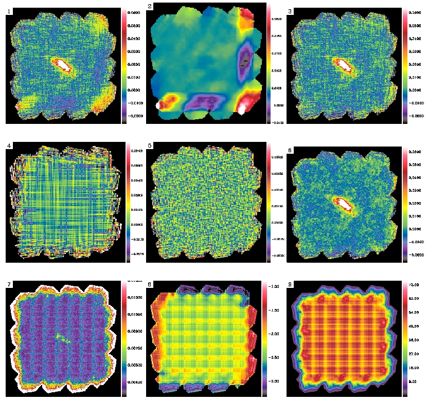
Figure 22: Successive steps of the processing of the NGC 4559 160 $\mu$m observations illustrated by maps. To accentuate the effects of the thermal drift in these illustrations, we have retained only the two obsids, and the first two scans in each, that immediately follow calibration blocks (Poglitsch et al. 2010), thus containing the strongest transients, on a total of four obsids with six scans each (but the numbers given in Table 1 apply to the full observations). The maps show the following: 1) data after subtraction of the full baselines; 2) average drift subtracted at the first iteration (notice the imprint of the transient following the observation of calibration sources at the start of each obsid, visible in the bottom and right edges of the map); 3) data after subtraction of the average drift; 4) individual drifts subtracted on a timescale of $27\times T_{c}$ ; 5) individual drifts subtracted on the minimum timescale $T_{c}$ ; 6) final map; 7) error map; 8) total drifts (dominated by baselines); 9) weight map. All maps are projected on a fine spatial grid (with pixels of FWHM/4 on a side), except maps 2, 4 and 5 that are projected on the coarser grid used for the processing.

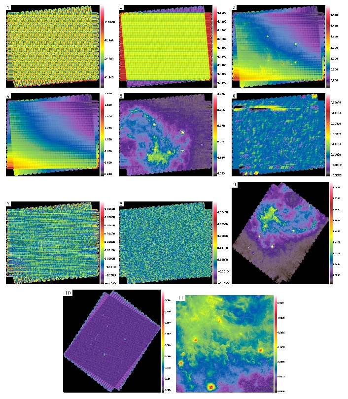
Figure 23: Successive steps of the processing of the Rosette 70 $\mu$m observations illustrated by maps, showing the following: 1) raw level-1 data; 2) simple zero-order baselines (flux calibration offsets); 3) data after subtraction of the zero-order baselines; 4) residual linear baselines derived from the redundancy; 5) data after subtraction of the residual baselines; 6) average drift subtracted at the first iteration (and glitches masked); 7) individual drifts subtracted on a timescale of $27\times T_{c}$ ; 8) individual drifts subtracted on a timescale of $3\times T_{c}$ ; 9) final map; 10) error map; 11) enlargement of a central portion of the final map (about $51^{\prime}$ on a side). Maps 1 to 8 are projected on a coarse spatial grid (with a pixel size equal to half the stability length), and maps 9 to 11 are projected on a fine grid (with pixels of FWHM/4 on a side). All the very compact sources are real. Notice that Scanamorphos was able to pick up the non-linear thermal drift near the end of the first scan, even though it has a low amplitude with respect to the sky signal (map 6).

5.2.3 Centaurus A (OD 233, obsid 1342188855 and 1342188856)

Centaurus A was observed in nominal mode as part of the Very Nearby Galaxies Survey (P.I. C. Wilson) and the spatial variations of its dust to gas mass ratio were analyzed by Parkin et al. (2012). Taking advantage of the fact that, for this galaxy, maps built from various methods were already available (courtesy of Marc Sauvage), we present a brief comparison of Scanamorphos with the two softwares fully implemented in HIPE for PACS: PhotProject, subtracting low-frequency noise by means of a high-pass filter, and MADmap, subtracting the uncorrelated noise with a matrix-inversion algorithm.

Figure 24 shows the final maps obtained for the two observed PACS bands, 70 and 160 $\mu$m, and Figure 25 shows the azimuthally-averaged surface brightness profiles. The respective advantages and disadvantages of the three methods are readily perceptible. We summarize them as follows:
1) PhotProject has no difficulty preserving compact sources, but filters out a non-negligible fraction of the extended emission. Even though a protective mask is applied to sources in the field before running the high-pass filter, this is insufficient to fully preserve the diffuse emission, because the brightness threshold of the mask cannot be set arbitrarily low. One can also notice residual short-timescale noise in the form of stripes, due to the fact that the filtering can be applied only to relatively large scales.
2) MADmap also preserves compact sources (except very bright ones, for which it is known to introduce artefacts in the shape of a cross-hair). Since it does not handle thermal drifts, however, it has difficulty restoring extended emission, and the sky structure on large spatial scales is not correct. On the other hand, the background noise on small scales is reduced to a very low level.
3) Scanamorphos preserves both compact and extended emission, and subtracts the low-frequency noise down to lower levels than the white noise on all timescales above $T_{c}$. The sky structure is less smooth than with the other two softwares, but this residual noise pattern remains well below the photometric errors, as shown in Section 4. Figure 25 shows that while there is essentially no difference between the three softwares at high surface brightnesses, Scanamorphos recovers more of the diffuse emission, especially at 160 $\mu$m.

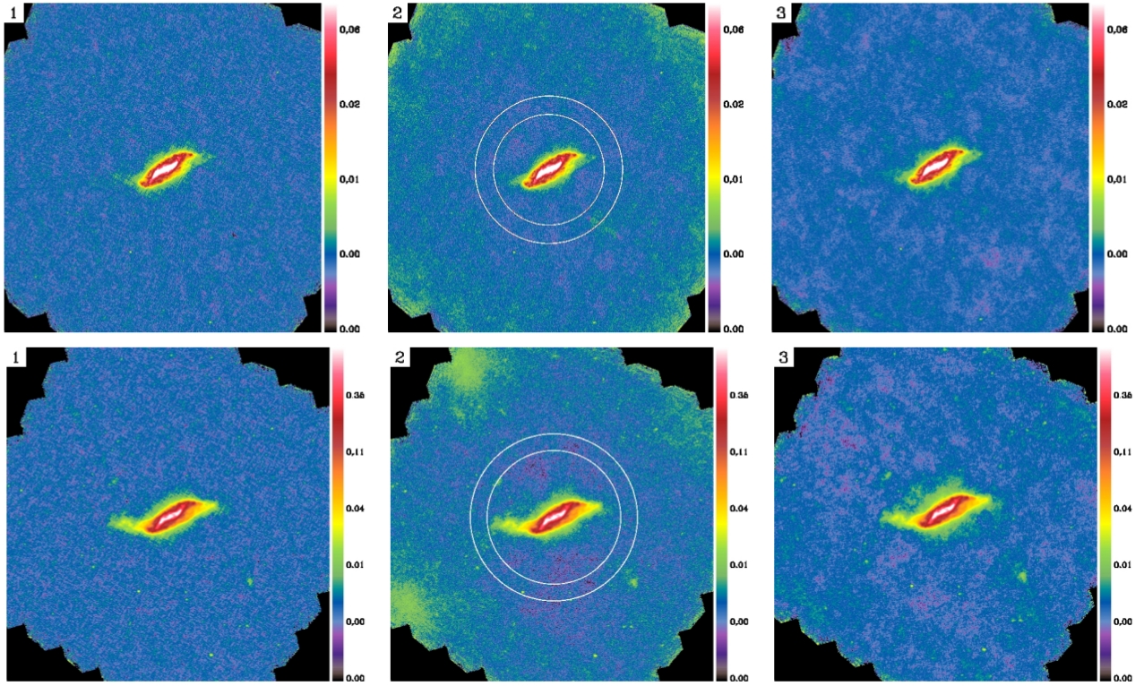
Figure 24: Maps produced by: 1) PhotProject at 70 $\mu$m; 2) MADmap at 70 $\mu$m; 3) Scanamorphos at 70 $\mu$m; 4) PhotProject at 160 $\mu$m; 5) MADmap at 160 $\mu$m; 6) Scanamorphos at 160 $\mu$m, in logarithmic scale. The pixel size is $2^{\prime\prime}$ at 70 $\mu$m and $4^{\prime\prime}$ at 160 $\mu$m. A brightness cut was applied to emphasize fainter structures (the results of the three softwares at higher surface brightnesses being similar). The concentric circles superimposed on the MADmap image indicate the region used to compute the background level in all maps.

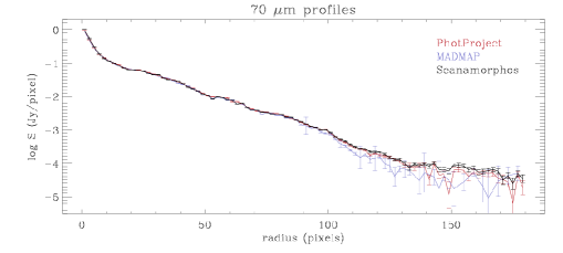
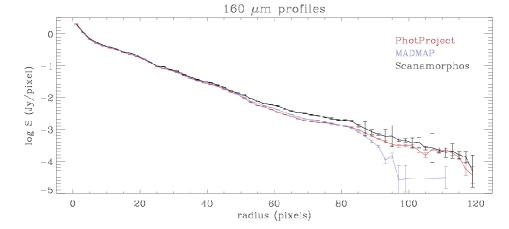
Figure 25: Surface brightness profiles of the Scanamorphos map (in black), the PhotProject map (in red) and the MADmap map (in blue). The radii of 180 pixels at 70 $\mu$m and 120 pixels at 160 $\mu$m correspond to the inner radius of the annulus shown in Fig. 24.

6 Final remarks

The foremost task of the algorithm described above is to subtract the low-frequency noise in scan observations made with bolometer arrays, or any photometers affected by the same type of noise. Its core principle is to use the redundancy in the observations, stemming from both the scanning strategy and the array structure, to derive the drifts from the data themselves, without using any noise model. It copes with both the thermal and non-thermal components of the noise (or more exactly, from the point of view of the algorithm, the average drift and the individual drifts; see Sect. 3.1), that are subtracted one after the other.

For each observation, the map size determines a boundary between what we have called long timescales (longer than the scan leg crossing time $T_{\rm leg}$) and short timescales (shorter than $T_{\rm leg}$). There is no fundamental difference between the drifts in these two frequency windows, but they call for distinct methods, because the long-timescale component is not adequately sampled by the data: subtracting it on the same principles as the short-timescale component would require a larger map.

The level of redundancy that is necessary to achieve our goals can be estimated in view of the coverage maps of Herschel observations. For those discussed in Section 5, the redundancy varies between 75 and 530 samples per square FWHM per scan pair (depending on the array structure and map parameters, and on the scan speed and sampling rate). The coverage can be rather inhomogeneous. Using pixels of size FWHM/4, a convenient fiducial value to remember is 10 samples per pixel per scan pair. The choice of the unit “scan pair” highlights the necessity to combine at least two scans separated by a large position angle difference in order to separate the drifts from the signal.

The simulations and examples of application presented here, in the context of Herschel observations, demonstrate that Scanamorphos is efficient at reducing the noise while preserving the flux and morphology of both compact sources and extended emission. It is robust with respect to small pointing and calibration errors, and we did not find any dataset from which it would not be able to produce a scientifically correct map. But since the redundancy is not infinite, and in some cases quite limited, correlated noise residuals can create artificial fluctuations of the sky emission (that remain well below the $3\sigma$ significance level). Scanamorphos is easily adaptable to progressively include corrections for new instrumental effects, as they become better understood, and has in particular been used to determine relative gain corrections for the SPIRE arrays (Appendix A).

Finally, we wish to remark on the impact of scanning strategies and on some adaptations that may be required for other instrument and telescope combinations: 1) The method to subtract the long-timescale drifts depends on the scan pattern. The algorithm in its current form is adapted when each scan can be decomposed into distinct scan legs (spanning the whole extent of the map in one direction), but would need to be modified for other types of scan patterns, for example rasters of spirals. 2) The thermal noise could be more complex for other instruments. For example, it could be significantly different from one subarray to the next, or among the parts of the array that are connected to different readout circuits. This is already partly accounted for in the subtraction of the long-timescale drifts, since this correction is made individually for each bolometer. The average drift subtraction on short timescales could also easily accommodate this level of complexity by splitting the signal into as many components as necessary, and doing the correction separately for each. It has in fact already been attempted, but was not found to bring any improvement for Herschel. 3) Our algorithm to subtract the thermal noise is in principle applicable to ground-based observations, and would be more effective than the customarily used filtering techniques. But to this effect the detectors need to be sampled at very high rates, at least a few times the knee frequency of the atmospheric noise. In other words, the unit length on which the correction can be achieved should be similar to or smaller than the atmospheric stability length.

7 Distribution

The Scanamorphos package can be retrieved from this URL: http://www2.iap.fr/users/roussel/herschel . It is possible to run the code with a minimal knowledge of IDL. Instructions for the installation and usage are included in the distribution, and example HIPE scripts and IDL commands to format the level-1 data and run Scanamorphos on the observations presented in Section 5 can be found in a subdirectory. Some advice and basic documentation, as well as an archive of all successive versions, can be found at the same URL.

The software can be run in visualization mode or in non-interactive mode. To avoid typing input parameters for each run, and process sequentially a large number of observations, a batch mode is also enabled. It is recommended to use this functionality only after gaining familiarity with the software.

Scanamorphos will be maintained for the duration of the Herschel mission and the archive phase.

Appendix A Gain corrections for SPIRE

From our tests made on various datasets with extended sources, and following up on an original idea by Darren Dowell (private communication), we have found necessary to apply some corrections to the gains of SPIRE bolometers. While the flux calibration of each array taken as a whole is exact, individual bolometers do not all have the same response (with a gain of one). This is because the flux calibration is built on point sources, and thus cannot account for the fact that the coupling of extended sources to each beam (with beam areas that are not uniform over the array) is different from that of point sources. The photometric corrections for extended sources that are given in the SPIRE Observers’ manual (in the “Flux density calibration” chapter) assume a unique beam, and neglect variations among bolometers. Corrections for non-uniform beams were first derived from a particular Galactic field (the Rosette nebula; see Sect. 5.1.1). The large brightness dynamic range over all spatial scales in this field enables the calibration of relative gains without having to worry about low-frequency drifts on short timescales, whose amplitude is completely negligible with respect to the effect of differential gains. We repeated the computation of gains, as explained below, using 17 different observations of bright complex fields, observed at low or nominal scan speed, and found consistent results in all cases. We could also check that there is an excellent correlation between the gains that we derived empirically and the measured beam areas of the individual bolometers, obtained from special calibration observations. The uncertainties associated with the latter observations are however much larger, which is why we adopt the empirical gains. These corrections have been successfully tested by the SPIRE ICC and have been included in branch 8 of HIPE. They should be applied in only one of the two softwares, HIPE or Scanamorphos, not in both.

The method to calibrate relative gains from science observations is the following. Baselines are first subtracted from the data, as explained in Section 3.4, and the resulting data are projected onto a map (with a pixel size of FWHM/4). Then, for each bolometer, we fit its brightness series as a linear function of the series simulated from the map, within a predefined brightness range. If the bolometer were perfectly calibrated, the fitted slope should be equal to one. The series of the bolometer is divided by this slope. The subtraction of baselines and division by slopes are then iterated a few times. The slopes are determined for each scan independently, and then averaged over all scans before being applied. At the end of the procedure, a relative gain is computed for each bolometer as the product of the slopes obtained in all iterations. The corrections are stored in files in the calibration directory and are applied by default to SPIRE data. Figure 26 shows the gain corrections as a function of bolometer index and Figure 27 as a function of bolometer position within the array. These gains are valid for branch 5 of the pipeline, and for all subsequent branches as long as the flux calibration changes only by a global factor. They are also available for branch 4, and will continue to be updated for each new flux calibration set if necessary (if the relative calibration is affected).

Global fluxes of extended sources are not changed by the application of the gains, since the map used as a reference for all bolometers is that initially built with the default flux calibration. On small scales, however, the effect may be non-negligible. For a given source, its exact amplitude is bound to depend on the position of the source relative to the array while it is being scanned, because the gains are a non-random function of bolometer position (Fig. 27). Although fluxes are not or only slightly changed, photometric errors have been found to be significantly decreased by the application of the gains.

Figure 26: Relative gains of valid SPIRE bolometers of the 250, 350, and 500 $\mu$m arrays, respectively, as a function of bolometer index, for the flux calibration set embedded in HIPE 5 and subsequent branches. The gains were derived from the observation of the Rosette nebula (Sect. 5.1.1) and 16 other bright complex fields. The error bars show the standard deviations among the fields.

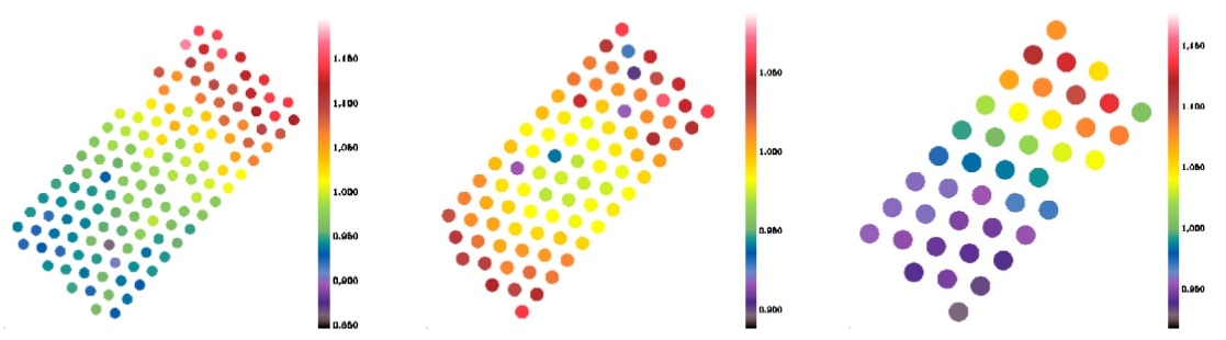
Figure 27: Maps of the relative gains of valid SPIRE bolometers of the 250, 350, and 500 $\mu$m arrays, respectively, for the flux calibration set embedded in HIPE 5 and subsequent branches. The arrays are oriented in the same way as when the scan direction is horizontal.

Appendix B Options

All the inputs and options are summarized in Table 2. They are described below. A full user guide, explaining how to set up the input data and describing the structure of the output, can be found in the online distribution.

B.1 Main options

- /jumps_pacs: If PACS data are affected by brightness discontinuities (see Sect. 3.6.1), this option can be used to detect the discontinuities and mask the affected samples. When Scanamorphos is run in iteractive mode, the user is required to visually check, and confirm or infirm each detection. The very unstable rows or bolometers are automatically detected and pre-filtered by the same module.
- /nothermal: If the thermal drift subtraction performed within HIPE is believed to be correct, the corresponding step in Scanamorphos can be bypassed.
- /noglitch: Likewise, if the deglitching performed within HIPE is trusted, it is possible to not perform it in Scanamorphos.
- /nogains (for SPIRE data only): If the HIPE version used locally does not match the flux calibration version for which the relative gains were derived, or if the gain correction was already performed within HIPE, the gain correction must not be performed in Scanamorphos.
- /parallel: For observations acquired in parallel mode, it is necessary to select the relevant option, because the smaller sampling rate implies that the frequency intervals used to compute the high-frequency noise amplitudes have to be adapted.
- /galactic: For observations of bright Galactic fields, it is highly recommended to use the relevant option, so that no sky structure can be removed by the baselines, as explained in Section 3.4. It should not be used for observations of diffuse Galactic structures, and in general for fields where the brightness gradients induced by the low-frequency noise are completely dominant over genuine brightness gradients of the sky. In case of doubt, it is advised to produce maps both with and without the /galactic option, and to compare them to decide which is the best strategy.
- /minimap: For fields observed in the mini-scan or small-map mode, that produces very small maps by definition, the relevant option should be selected in order to deactivate the destriping and average drift subtraction modules, since there are not enough resolution elements with nominal coverage across the map to make these corrections necessary and accurate. These corrections may also need to be deactivated (by selecting the /minimap option) when there are only two or three scan legs per scan. As above, in case of doubt, it is advised to produce maps both with and without the /minimap option and to compare them.
- /nocross: For observations in which the nominal coverage consists of scans taken in only one direction, some adaptations are necessary, and in particular no destriping can be performed. Note that such observations are not recommended. This option is provided to qualitatively assess observations that are not completed yet, but is not guaranteed to produce science-grade maps.

In visualization mode (with the /visu or /debug option), it is possible to inspect the average drift series and choose to apply the correction or not. When the nonlinear component of the thermal drift is negligible, and consequently the average drift amplitude very small (with respect to the high-frequency noise), the correction may introduce noise. In case of doubt, it is best to do the processing once with the average drift subtraction, and a second time without this correction, to compare the final maps and to select the best one.

B.2 Non-default astrometry

By default, the astrometry and spatial grid are determined from the input scans. The user has however the latitude to change the spatial grid or request that only a portion of the entire field be processed and mapped:
1) by supplying a reference fits header (in the form of an IDL string array). In that case, the astrometry is taken entirely from the header. With this option, only one array should be processed at a time. Note that it is usable in batch mode, and then requires the header to be in the form of an IDL save file, containing a variable named exactly hdr_ref .
2) by supplying a three-element array containing the central coordinates and minimum radius of a subfield to be excised from the data (all in degrees): $cutout=[ra_{center},dec_{center},radius]$

It is also possible to specify astrometric offsets for each scan (angular distances in arcsec) with the offset_ra_as and offset_dec_as parameters.

Table 2: Summary of inputs and options

auxiliary files
scanlist_spire	ascii file containing the directory and file names of the input scans
scanlist_pacs	idem
command line keywords and parameters
spire	select to process SPIRE observations
pacs	select to process PACS observations
nobs	for PACS: number of distinct obsids
visu	select to visualize intermediate results and stop after each major step
vis_traject	select to check that scan directions are alternating correctly
debug	detailed visualizations, for experts only
version	select to print the software and SPIRE relative gains versions
jumps_pacs	select to detect and mask brightness discontinuities in PACS data
nothermal	select to bypass the short-timescale average drift correction
noglitch	select to bypass glitch masking and asteroid detection
nogains	select if the gain version does not match the local flux calibration version
	or if the relative gain correction has already been applied in HIPE (SPIRE)
parallel	select in case of parallel-mode observations
galactic	select in case of very bright Galactic field or similar dataset
minimap	select in case of mini-scan or small-map mode
flat	select to force the sky background to be flat
nocross	select for observations consisting of scans in a single direction or non-overlapping
hdr_ref	reference header to enforce the same astrometry
	(IDL string array or IDL save file containing a variable named “hdr_ref”)
cutout	central RA and DEC coordinates and radius of the subfield to be processed and mapped
nblocks	number of spatial blocks the field of view will be sliced into
block_start	index of the first spatial block to be processed, when nblocks $>1$
one_plane_fits	select to save each plane in a separate fits file
offset_ra_as	right ascension offsets (angular distances) to be applied to the map coordinates (one for each scan)
offset_dec_as	declination offsets (angular distances) to be applied to the map coordinates (one for each scan)
inputs at the prompt
output directory	directory where final maps and intermediate variables will be stored
output FITS file root	full file name = file root + instrument + wavelength + block index + “.fits”
detector arrays	choose only one for PACS and between one and three for SPIRE
map orientation	binary choice: orientation of the first scan (default), or standard astronomical orientation
pixel size	in arcsec, equal to FWHM/4 by default
turnaround data	option to reject turnaround data from final map
nobs	for PACS: if not supplied at the command line

References

- André et al. (2008) André, P., Minier, V., Gallais, P., Reveret, V., Le Pennec, J., Rodriguez, L., et al. 2008, A&A, 490, L27
- Aniano et al. (2011) Aniano, G, Draine, B.T., Gordon, K.D., & Sandstrom, K. 2011, PASP, 123, 1218
- Ashdown et al. (2007) Ashdown, M.A., Baccigalupi, C., Balbi, A., Bartlett, J.G., Borrill, J., Cantalupo, C., et al. 2007, A&A, 467, 761
- Billot (2008) Billot, N. 2008, PhD thesis, Université Paris-Sud XI, arXiv:0808.3958
- Billot et al. (2006) Billot, N., Agnèse, P., Auguères, J.L., et al. 2006, SPIE 6265, 9B
- Cantalupo (2010) Cantalupo, C.M., Borrill, J.D., Jaffe, A.H., Kisner, T.S., & Stompor, R. 2010, ApJS, 187, 212
- Davies et al. (2010) Davies, J.I., Baes, M., Bendo, G.J., Bianchi, S., Bomans, D.J., Boselli, A., et al. 2010, A&A, 518, L48
- Dowell et al. (2010) Dowell, C.D., Pohlen, M., Pearson, C., Griffin, M., Lim, T., et al. 2010, SPIE 7731, 101
- Eales et al. (2010) Eales, S., Dunne, L., Clements, D., Cooray, A., De Zotti, G., et al. 2010, PASP, 122, 499
- Emerson et al. (1979) Emerson, D.T., Klein, U., & Haslam, C.G. 1979, A&A, 76, 92
- Fruchter & Hook (2002) Fruchter, A.S., & Hook, R.N. 2002, PASP, 114, 144
- Galametz et al. (2010) Galametz, M., Madden, S.C., Galliano, F., Hony, S., Sauvage, M., Pohlen, M., et al. 2010, A&A, 518, L55
- Griffin et al. (2010) Griffin, M., et al. 2010, A&A, 518, L3
- Hanisch et al. (2001) Hanisch, R.J., Farris, A., Greisen, E.W., et al. 2001, A&A, 376, 359
- Kennicutt et al. (2003) Kennicutt, R.C., et al. 2003, PASP, 115, 928
- Kennicutt et al. (2011) Kennicutt, R.C., et al. 2011, PASP, 123, 1347
- Kovács (2008a) Kovács, A. 2008, SPIE, 7020, 5
- Kovács (2008b) Kovács, A. 2008, SPIE, 7020, 45
- Minier et al. (2009) Minier, V., André, P., Bergman, P., Motte, F., Wyrowski, F., Le Pennec, J., et al. 2009, A&A, 501, L1
- Motte et al. (2010) Motte, F., Zavagno, A., Bontemps, S., et al. 2010, A&A, 518, L77
- Motte et al. (2007) Motte, F., Bontemps, S., Schilke, P., Schneider, N., Menten, K.M., & Broguière, D. 2007, A&A, 476, 1243
- Ott (2010) Ott, S. 2010, ASP Conference Series, 434, 139 (ADASS XIX)
- Parkin et al. (2012) Parkin, T.J., Wilson, C.D., Foyle, K., et al. 2012, MNRAS, 422, 2291
- Pilbratt et al. (2010) Pilbratt, G.L., Riedinger, J.R., Passvogel, T., et al. 2010, A&A, 518, L1
- Poglitsch et al. (2010) Poglitsch, A., Waelkens, C., Geis, N., Feuchtgruber, H., Vandenbussche, B., et al. 2010, A&A, 518, L2
- Russeil et al. (2012) Russeil, D., Schneider, N., Anderson, L. D. et al. 2013, A&A, 554, A42
- Swinyard et al. (2010) Swinyard, B.M., Ade, P., Baluteau, J.P., et al. 2010, A&A, 518, L4
- Talvard et al. (2006) Talvard, M., André, P., Rodriguez, L., Minier, V., Benoit, A., Leriche, B., et al. 2006, SPIE, 6275, 2
- Waskett et al. (2007) Waskett, T.J., Sibthorpe, B., Griffin, M.J., & Chanial, P.F. 2007, MNRAS, 381, 1583
- Wells et al. (1981) Wells, D.C., Greisen, E.W., & Harten, R.H. 1981, A&AS, 44, 363
- Wieprecht et al. (2009) Wieprecht, E., Schreiber, J., de Jong, J., Jacobson, J., Liu, C., Morien, B., Wetzstein, M., et al. 2009, ASPC, 411, 531