A survey of nulling pulsars using the Giant Meterwave Radio Telescope

Abstract

Several pulsars show sudden cessation of pulsed emission, which is known as pulsar nulling. In this paper, the nulling behaviour of 15 pulsars is presented. The nulling fractions of these pulsars, along with the degree of reduction in the pulse energy during the null phase, are reported for these pulsars. A quasi-periodic null-burst pattern is reported for PSR J1738$-$2330. The distributions of lengths of the null and the burst phases as well as the typical nulling time scales are estimated for eight strong pulsars. The nulling pattern of four pulsars with similar nulling fraction are found to be different from each other, suggesting that the fraction of null pulses does not quantify the nulling behaviour of a pulsar in full detail. Analysis of these distributions also indicate that while the null and the burst pulses occur in groups, the underlying distribution of the interval between a transition from the null to the burst phase and vice verse appears to be similar to that of a stochastic Poisson point process.

1 Introduction

The abrupt cessation of pulsed radio emission for several pulse periods, exhibited by some pulsars, has remained unexplained despite the discovery of this phenomenon in many radio pulsars. This phenomenon, called pulse nulling, was first discovered in four pulsars in 1970. Subsequent studies have revealed pulse nulling in about 100 pulsars to date (Backer 1970; Hesse & Wielebinski 1974; Ritchings 1976; Biggs 1992; Vivekanand 1995; Wang et al. 2007). The degree and form of pulse nulling varies from one pulsar to another. On one hand, there are pulsars such as PSR B0826$-$34 (Durdin et al. 1979), which null most of the time, and PSR B1931+24 (Kramer et al. 2006), which exhibits no radio emission for 2 $-$ 4 weeks. In contrast, pulsars such as PSR B0809+74 show a small degree of nulling (Lyne & Ashworth 1983). Pulse nulling is frequent in pulsars such as PSR B1112+50, while it is very sporadic in PSR B1642$-$03 (Ritchings 1976).

The fraction of pulses with no detectable emission is known as the nulling fraction (NF) and is a measure of the degree of nulling in a pulsar. However, NF does not specify the duration of individual nulls, nor does it specify how the nulls are spaced in time. Although some attempts of characterizing patterns in pulse nulling were made in the previous studies (Backer 1970; Ritchings 1976; Janssen & van Leeuwen 2004; Kloumann & Rankin 2010), not many pulsars have been studied for systematic patterns in nulling, partly because these require sensitive and long observations.

Recent discoveries suggest that nulling pulsars with similar NF may have different null durations. These include intermittent pulsars, such as PSR B1931+24 (Kramer et al. 2006) and PSR J1832+0029 (Lyne 2009), and the rotating radio transients (RRATs), which show no pulsed emission between single burst of emission (McLaughlin et al. 2006). These pulsars also show extreme degree of nulling similar to few classical nulling pulsars. PSR B1931+24 exhibits radio pulsations for 5 to 10 days followed by an absence of pulsations for 25 to 35 days (Kramer et al. 2006). If the cessation of radio emission in this pulsar is interpreted as a null, it has a NF of about $\sim$75 percent similar to PSR J1502$-$5653 (Wang et al. 2007). Yet the latter shows nulls with a typical duration of few tens of seconds in contrast to a much longer duration for PSR B1931+24. A similar conclusion can be drawn by comparing RRATs with classical high NF pulsars. While this leads to the expectation that pulsars with similar NF may have different nulling timescales, no systematic study of this aspect of nulling is available to the best of our knowledge. In this paper, a modest attempt to investigate this is initiated.

Pulse nulling was usually believed to be a random phenomenon (Ritchings 1976; Biggs 1992). However, recent studies indicate a non-random nulling behaviour for a few classical nulling pulsars (Redman and Rankin 2009; Kloumann and Rankin 2010). Redman and Rankin (2009) also report random nulling behaviour for at least 4 out of 18 pulsars in their sample. Therefore, it is not clear if non-randomness in the sense defined in Redman and Rankin (2009) is seen in most nulling pulsars and such a study needs to be extended to more nulling pulsars. This issue is investigated in this paper with a distinct set of nulling pulsars.

In this paper, we present observations of 15 pulsars, carried out using the Giant Meterwave Radio Telescope (GMRT) at 325 and 610 MHz. Among these, five were discovered in the Parkes multibeam pulsar survey (PKSMB; Manchester et al. 2001; Morris et al. 2002; Kramer et al. 2003; Lorimer et al. 2006), which have no previously reported nulling behaviour. Rest of the sample consists of well known strong nulling pulsars. The observations and analysis techniques are described in Section 2. In Section 3, interesting features of the nulling behaviour for a few pulsars are discussed along with estimates of their NF and the reduction in the pulsed energy during the null phase. A comparison of the null length and burst length distributions for pulsars, which have similar NF, is presented in Section 4 and a discussion on the randomness of nulls is presented in Section 5. The expected time-scales for the null and burst durations are presented in Section 6. Finally, the implications of these results are discussed in Section 7 and the conclusions are presented in Section 8.

Figure 1: Integrated pulse profiles of six pulsars (five of which were discovered in PKSMB), with no previously reported low frequency study, at 325/610 MHz. The profile for PSR J1738$-$2330 (dashed line) was obtained from data at 325 MHz, while the other profiles (continuous line) were obtained from data at 610 MHz. All the profiles are plotted over equal phase interval (indicated at the bottom of the figure) for comparison.

2 Observations and Results

This survey of a sample of nulling pulsars was conducted using the GMRT (Swarup et al. 1991). The observations were carried out at 325 and 610 MHz using a total time of 60 hrs from 2008 November 9 to 2009 August 21. For our observations, the GMRT correlator was used as a digital filterbank to obtain 256 spectral channels, each having a bandwidth of 62.5 KHz, across the 16 MHz bandpass for each polarization received from the 30 antennas of GMRT. The digitized signals from typically 14 to 20 GMRT antennas were added in phase (the GMRT was used as a phased array) forming a coherent sum of signals with the GMRT Array Combiner (GAC). Then, the summed signals were detected in each channel. The detected powers in each channel were then acquired into 16-bit registers every 16 $\mu$s after summing the two polarizations in a digital backend and were accumulated before being written to an output buffer to reduce the data volume. The data were then acquired using a data acquisition card and recorded to a tape for off-line processing. The effective sampling time for this configuration, used for most of the survey, was 1 msec.

In the off-line processing, the data were first dedispersed and then folded to typically 256 phase bins across the topocentric pulse period using a publicly available package SIGPROC to obtain an integrated profile for each pulsar. Our sample included six pulsars (among which five were discovered in PKSMB pulsar survey) with no previously reported low frequency studies. The integrated profiles for these six pulsars are shown in Figure 1. These profiles at low radio frequencies are being reported for the first time to the best of our knowledge. Two of these pulsars, PSRs J1701$-$3726 and J1901+0413, exhibit marked scattering tail in their profiles at 610 MHz, while scattering tails are also apparent in two other pulsars, PSRs J1639$-$4359 and J1715$-$4034, although not as prominent as in the case of the former two pulsars.

The dedispersed data were then folded to typically 256 phase bins across the topocentric pulse period for each period to form a single pulse sequence. For few pulsars with low intensity single pulses, a fixed number, N, of successive pulses (indicated within parentheses in Column 10 of Table 1) in the single pulse data were averaged to form average pulse for every block of N single pulses (hereafter called subintegration), to obtain sufficient signal to noise ratio (i.e. S/N $\geq$ 5 for each subintegration). Pulses affected by radio frequency interference (RFI), were removed before the NF analysis. The NF for each pulsar was then obtained using a procedure similar to that used for detecting pulse nulling in single pulse sequences (Ritchings 1976; Vivekanand 1995). A baseline, estimated using bins away from the on-pulse bins, was subtracted from the data for each pulse. The total energy for each pulse in the on-pulse window and the off-pulse window (both with equal number of bins) was calculated from the baseline subtracted data. The energies thus obtained as a function of period number form an on-pulse energy (ONPE) sequence and off-pulse energy (OFPE) sequence. Next, the ONPE and OFPE were scaled by the average on-pulse energy, calculated for every block of 200 periods from ONPE, to compensate for variations due to inter-stellar scintillations. The normalized ONPE and OFPE were then binned to an appropriate number of energy bins depending upon the available S/N for a given pulsar. The fraction of total pulses per energy bin was plotted as a histogram as shown in Figure 2. An excess at zero energy in the on-pulse energy distribution indicates the fraction of nulled pulses or NF of the pulsar. This can be estimated by removing a scaled version of off-pulse energy distribution (modeled as a Gaussian) at zero energy from the on-pulse distribution. As the null and burst pulse distributions are not well separated for most of our pulsars, such a fit of the off-pulse energy distribution, modeled as a Gaussian, will have a corresponding error while scaling the on-pulse energy distribution near the zero pulse energy. This is reflected in the quoted errors on the NFs given in the parentheses in Column 6 of Table 1.

Three pulsars in our sample were weak. Hence, consecutive pulses were added (indicated inside parentheses of Column 10 in Table 1) to improve the S/N ratio. NF for these three pulsars, obtained using the above mentioned method on data averaged over given number of consecutive periods (subintegration), will be an under estimate. Hence, only the lower limits on the NFs for these pulsars are presented in Table 1.

Only upper limits on the NFs could be estimated for three pulsars in the sample. Two of these were weak pulsars with significantly low nulling. Estimation of the lower limits on the NFs (as explained in the previous paragraph) was not possible as averaging over consecutive periods resulted in detection of emission for every subintegration giving a NF of zero. However, some of the single pulses in a subintegration may well have been nulled pulses. To estimate an upper limit on the fraction of such pulses for these two pulsars, we arranged all the single pulses in the ascending order of their on-pulse energy. A threshold was moved from high to low on-pulse energy end till the pulses below the threshold did not show a collective profile with a pulse at significance greater than 3 times the root mean square deviation (RMS). All the pulses below such threshold were tagged as null pulses. The fraction of these pulses give an estimate for the upper limit on the NF and this limit is presented for these two pulsars in Column 6 of Table 1. The reason for the upper limit on the NF for the remaining pulsar, PSR J1725$-$4043, is explained in Section 3.

Figure 2: Normalized histogram of on-pulse (solid line) and off-pulse (dot-dot-dashed line) energies, normalized as explained in the text, for PSR B2319+60. The residuals after the subtraction of a scaled version of off-pulse distribution from the on-pulse distribution are shown with dashed line. The dotted vertical line is visually selected threshold at the point where null and burst pulse distributions cross each other in on-pulse histogram.

The degree, $\eta$, by which the radio emission from a nulling pulsar declines during the nulls can be obtained by forming the average profiles of the pulsar for burst and null pulses separately. A threshold energy, decided by examining the on-pulse and off-pulse energy distributions of the pulsar, was used to separate burst and null pulses as shown in Figure 2. If the distribution of burst and null pulses are not well separated, such a threshold will cause few low energy burst pulses to be tagged as null pulses and vice-verse. To identify these low energy burst pulses among null pulses, we arranged all null pulses in ascending order of their on-pulse energy. Pulses were removed manually from the high energy end till the null pulse profile, averaged over the remaining null pulses, did not show any profile component with more than 3 times the RMS. These pulses, from the high energy end, were tagged as burst pulses. Similarly, burst pulses were also arranged in ascending order of their on-pulse energy. Pulses from the lower end of the on-pulse energy, which did not form an average pulse profile with a significant pulse ($\geq$ 3 times the RMS), were also removed and tagged as null pulses. We calculated $\eta$ for a pulsar in a manner similar to that described in Vivekanand & Joshi (1997). First, the total energy in the on-pulse bins for the burst pulse profile was obtained. Then, an upper limit, estimated as three times the RMS, was obtained on the detectable emission in the null pulse profile. The ratio between these two quantities is defined as $\eta$ (Equation 1).

$$\eta~{}=~{}\frac{\sum\limits^{N}_{i=1}P_{bpulse}(i)}{3\times RMS_{npulse}}$$ (1)

where
P_bpulse = Intensity in i^th bin for the on-pulse window of the burst pulse profile
RMS_npulse = RMS estimated over the on-pulse window of the null pulse profile
N = Number of bins in the on-pulse window

The errors given in the parentheses in Column 8 were estimated as 3 times the off-pulse RMS in the burst pulse profile. We are reporting $\eta$ for 11 pulsars in our sample for the first time.

The results of our analysis for the sample of pulsars in this study are presented in Table 1. The Table presents some of the basic parameters for the observed pulsars (i.e. Column 3 : Period, Column 4 : DM and Column 5 : Flux density at 1420 MHz). It also presents NFs with the corresponding error in the parentheses (i.e. Column 6) for all the pulsars of our sample. The previously reported NFs (i.e. Column 7) for some pulsars are also listed for comparison and our results are consistent with those reported earlier for these pulsars. NFs are being reported for the first time in five pulsars, which were discovered in PKSMB survey. For 11 pulsars in our sample, estimates for $\eta$ are reported for the first time (i.e. Column 8).

To investigate the time scales of the null and the burst phase (i.e. normal emission), the single pulse sequences for eight pulsars were examined. These pulsars show high S/N (i.e. $\geq$ 5) for single burst pulses. Hence, null and burst pulses can be separated easily using the above mentioned method. The null lengths and burst lengths as well as the total number of uninterrupted sequences of null and burst phases were obtained from this examination of data. The null length histogram (NLH) and burst length histogram (BLH) for these eight pulsars, are shown in Figure 5.

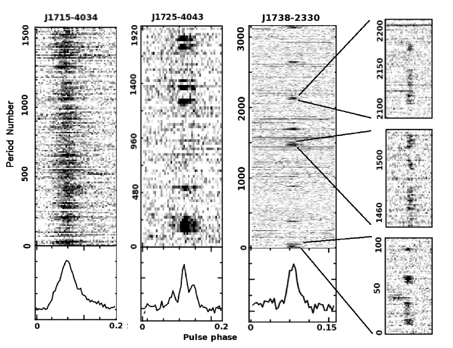
Figure 3: The modulation of pulsar energy in single pulses for three pulsars. Successive 10, 24 and 5 periods were averaged as a subintegration. The resulting subintegrations are plotted as gray-scale intensities for PSRs J1715$-$4034, J1725$-$4043 and J1738$-$2330 respectively for the entire stretch of observed data. Bottom panel of each plot shows the integrated profiles for the respective pulsars. The insets, where individual periods without any averaging are plotted, show 3 burst pulse bunches for PSR J1738$-$2330.

Table 1: Parameters for the pulsars, observed in this survey, along with the obtained nulling fraction (NF) and reduction in the pulse energy during the null phase ($\eta$). Columns give pulsar name at 2000 and 1950 epochs, period (P)^a, dispersion measure (DM)^a, flux density at 1400 MHz (S1400)^a, NF (as defined in text) obtained in this study, NF reported previously, estimate of $\eta$ (as defined in text) obtained in this study, number of runs and the number of pulses used (N) along with the number of contiguous pulses integrated (given in parentheses) for the analysis. The error bars on obtained values of NF and $\eta$ are indicated after the estimates by the number in the round parentheses and represent 3 times the standard deviation errors. The references for the previously reported NF in Column 7 are as follows: (1) Lyne & Ashworth 1986 (2) Biggs 1992 (3) Ritchings 1976 (4) Herfindal & Rankin 2009 (5) Wang et al. 2007

J2000	B1950	Period	DM	S1400	Obtained	Known	$\eta$	Number of	N (Sub-integration)
Name	Name				NF	NF		Runs
		(s)	(pc/cm3)	(mJy)	(%)	(%)	$-$	$-$	$-$
J0814+7429	B0809+74	1.292241	06.1	10.0	1.0(0.4)	1.42(0.02) [1]	172.0(0.5)	246	13766 (1)
J0820$-$1350	B0818$-$13	1.238130	40.9	7.0	0.9(1.8)	1.01(0.01) [1]	4.2(0.2)	114	3341 (1)
J0837$-$4135	B0835$-$41	0.751624	147.2	16.0	1.7(1.2)	$\leq$1.2 [2]	15.7(0.2)	148	3335 (1)
J1115+5030	B1112+50	1.656439	9.2	3.0	64(6)	60(5) [3]	44.7(0.2)	1270	2634 (1)
J1639$-$4359	$-$	0.587559	258.9	0.92	$\leq$0.1	$-$	$-$	$-$	13034 (1)
J1701$-$3726	$-$	2.454609	303.4	2.9	19(6)	$\geq$14 [5]	6.4(0.2)	$-$	2464 (1)
J1715$-$4034	$-$	2.072153	254.0	1.60	$\geq$6	$-$	$-$	$-$	1591 (16)
J1725$-$4043	$-$	1.465071	203.0	0.34	$\leq$70	$-$	$-$	$-$	2481 (24)
J1738$-$2330	$-$	1.978847	99.3	0.48	$\geq$69	$-$	5.3(0.3)	$-$	2178 (5)
J1901+0413	$-$	2.663080	352.0	1.10	$\leq$6	$-$	$-$	$-$	2605 (1)
J2022+2854	B2020+28	0.343402	24.6	38	0.2(1.6)	$\leq$ 3 [3]	2.5(0.2)	$-$	8039 (1)
J2022+5154	B2021+51	0.529196	22.6	27.0	1.4(0.7)	$\leq$5 [3]	2.6(0.2)	24	1326 (1)
J2037+1942	B2034+19	2.074377	36.0	$-$	$\geq$26	44(4) [4]	6.4(0.1)	672	1618 (3)
J2113+4644	B2111+46	1.014685	141.3	19.0	21(4)	12.5(2.5) [3]	14.9(0.3)	290	6208 (1)
J2321+6024	B2319+60	2.256488	94.6	12.0	29(1)	25(5) [3]	115.8(0.4)	450	1795 (1)

^a ATNF Catalogue : http://www.atnf.csiro.au/research/pulsar/psrcat/

3 Nulling behaviour of individual pulsars

The salient features of the nulling behaviour of a few individual pulsars are discussed below

PSR J1715$-$4034 : This pulsar was discovered in PKSMB (Kramer et al. 2003). No nulling behaviour has been reported previously for this pulsar. Width of the pulses is significantly modulated as seen in Figure 3. There are two components in the integrated profile at 1420 MHz (Kramer et al. 2003), which are difficult to identify at 610 MHz because of scatter-broadening. Independent modulation in these components can cause this apparent change in the pulse width.

PSR J1725$-$4043 : This is also one of the pulsars discovered in PKSMB (Kramer et al. 2003) with no previously reported nulling behaviour. Its integrated profile at 610 MHz exhibits three narrow components - one strong central component with weak trailing and leading components. Single pulse data were averaged over successive pulses to form average profiles for every block of 24 single pulses (subintegrations). A gray-scale plot of these subintegrations as well as the integrated profile for this pulsar is shown in Figure 3. Visual inspection of the gray-scale plot shows emission bunches of 50 to 200 strong pulses, which correspond to the normal integrated profile (hereafter referred as Mode A - for example subintegrations 120 to 264 in Figure 3). After adding all the subintegrations during the null phase, separated by visual inspection, a weak profile (hereafter referred as Mode B - for example subintegrations 264 to 480 in Figure 3), different from the normal integrated profile (Mode A), is obtained. The integrated profiles for the two modes are shown in Figure 4. Although the two profiles are similar in shape with distinct three components, Mode B profile shows relatively stronger trailing component (Figure 4). Hence, it appears that the pulsar shows sporadic emission with two distinct modes.

Manual inspection of the single pulses, forming the null subintegrations, reveals weak individual pulses among nulled pulses. Hence, it is difficult to identify null pulses as these could be low intensity Mode B pulses. Pulsar spends 30% of time in Mode A emission. The remaining 70% could be combination of null pulses and Mode B emission. Hence, only an upper limit on the NF for this pulsar is quoted in Table 1.

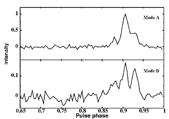
Figure 4: Integrated pulse profiles for Mode A and Mode B of PSR J1725$-$4043. The ordinate is in arbitrary units and was obtained after scaling the two profiles by the peak intensity of the Mode A profile. The Mode B is around 10 times weaker than Mode A.

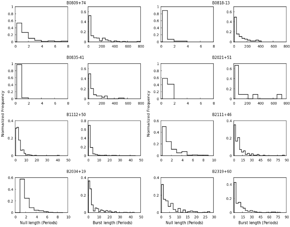
Figure 5: Null length and burst length histograms of eight pulsars in the sample. The histogram in the left panel for each pulsar shows the distribution of observed null lengths, while that on the right panel shows the distribution of observed burst lengths.

PSR J1738$-$2330 : This is another pulsar discovered in the PKSMB (Lorimer et al. 2006). In our survey, it was observed at 325 MHz. The pulsar seems to have quasi-periodic bursts, with an average duration of around 50 to 100 periods, interspersed with nulls of around 300 to 400 periods. This interesting single pulse behaviour in this pulsar is evident in Figure 3, where a gray scale plot, with 5 successive single pulses integrated, is shown. We note that the bursts are quasi-periodic, and that a phase-resolved frequency spectrum (Figure 6) shows power at 0.0019 cycles/period and 0.0028 cycles/period, which correspond to periodicities of approximately 525 and 350 periods, respectively. This quasi-periodic behaviour is similar to PSR B1931+24 but with much shorter time scale.

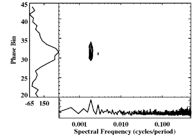
Figure 6: The phase-resolved spectra for PSR J1738$-$2330. The contours in the main panel show spectra for bins 20 to 44 across the on-pulse window. The left panel shows the integrated profile for these pulse phases, whereas the bottom panel shows the averaged spectra for all the on-pulse phases (bins 28 to 38). The spectra in the bottom panel and in contours are shown with the abscissa plotted in a logarithmic scale upto the Nyquist frequency.

Close examination of single pulses suggests that the bursts typically consist of a sequence of a 20 to 30 period burst followed by 2 short bursts of 5 to 10 pulses. These three bursts are separated by shorter nulls of about 10 to 25 pulses. The overall burst pattern is itself separated by around 400 pulse period nulls. Three examples of this burst pattern are indicated in Figure 3. However, our S/N was too low to confirm this with high significance. More sensitive and long observations in future may be useful to resolve burst pattern and periodicities.

PSR B2020+28 : This is one of the well studied pulsars. The pulse profile shows two strong components, but this pulsar was classified as triple profile class pulsar because of the prominent saddle region between the two components (Rankin et al. 1989). Interestingly, the emission in the individual profile components reduces significantly for a fraction of pulses, which is different for the two components. Our time resolution was not sufficient to identify the saddle region clearly so we were able to estimate NF for two components only. The estimated NF for the leading component is 3.5 $\pm$ 0.8 % and $\eta$ is around 9.7. The estimated NF for the trailing component is 9 $\pm$ 1 % and $\eta$ is around 21, suggesting that at least the trailing component shows a nulling behaviour similar to a regular nulling pulsar. Both these individual NFs were significantly higher than the overall NF (Table 1).

PSR B2111+46 : This pulsar has a multicomponent profile, classified as a triple component profile class by Rankin et al. (1989). Like PSR B2020+28, the fraction of pulses for which emission is not detected varies from component to component. For the core component, NF was estimated to be of 26 $\pm$ 2 %, slightly higher than the NF of the entire pulse (Table 1). The estimated $\eta$ value for this component is around 56. For the leading component, NF was found to be 53 $\pm$ 5, almost double the NF for the entire pulse. NLH and BLH considering the emission in the entire pulse are reported here for the first time for this pulsar. NLH shows 50% of nulls are single period nulls while other 50% are gradually distributed up to 10 periods.

4 Comparing nulling behaviour

In this study, NLH and BLH were obtained for 8 out of the 15 pulsars observed. This allows a comparison of null lengths for these pulsars, particularly for PSRs B0809+74, B0818$-$13, B0835$-$41 and B2021+51, all of which have similar NF of around 1%. Visual inspection of all single pulses for these 4 pulsars suggests that the pattern of arrangement of nulls within the burst differs for each of these pulsars and motivates a quantitative study. To investigate this, the NLHs and BLHs for these pulsars were examined. While the BLHs are similar for all the 4 pulsars, the NLHs show significant differences. While PSRs B0835$-$41 and B2021+51 show only single and double period nulls, PSRs B0809+74 and B0818$-$13 show nulls of longer durations as well.

To quantify these differences, a two sample Kolmogorov-Smirnov (KS) test (Press et al. 2001) was carried out for the four pulsars mentioned above. KS-test is a non-parametric distribution free test, applicable to unbinned data. KS-test provides a statistic, D, which is the maximum difference between the two cumulative distribution functions (CDFs). To compare the null length distribution of two pulsars, we formed their CDFs from the observed unbinned null length sequences. We found D from their CDFs and estimated the rejection probability of null hypothesis, which assumes that the measured distributions are drawn from the same underlying distribution. The results of this test are given in Table 2 for each pair of the four pulsars. The null hypothesis is rejected for all pairs with high significance (except for the comparison of null lengths for PSRs B0818$-$13 and B0835$-$41, where the significance is marginally smaller). Thus, the nulling patterns differ between each of the four pulsars even though they have the same NF. This kind of differences are not only seen in pulsars with small NF, but also in pulsars with larger NF. For example, PSRs B2319+60 and B2034+19 have NF $\sim$ 30% but their NLH are different. A KS-test (result not shown in the table) once again rejects the null hypothesis with high significance. Likewise, NLH for PSRs B2111+46 also differ with PSRs B2319+60 and B2034+19. However, as these pulsars have slightly different NFs, it is difficult to draw a strong conclusion from these data.

5 Do nulls occur randomly ?

Previous studies (Redman and Rankin 2009; Kloumann and Rankin 2010) indicated that nulling may not be random. To test the above premise, non-randomness tests were carried out on our data for 8 pulsars where it was possible to obtain NLH and BLH.

If the null pulses of a pulsar are characterized by an independent identically distributed (iid) random variable, for which NF represents the proportion statistics, then one can Monte-Carlo simulate synthetic data sets using a random number generator (Press et al. 2001). We simulated around 10,000 random one-zero time series of the same length as that of the sequence of the observed pulses for each pulsar with a given NF. A distribution of null and burst length was derived from the synthetic data set. If the underlying distribution of observed null lengths does not differ from the the simulated distribution with high significance, then it can be concluded that the observed nulls are sampled from a distribution characterizing such an iid random variable, for which NF represents the proportion statistics. The above premise can be tested by carrying out a one sample KS-test (Press et al. 2001). As explained in the earlier section, KS-test provides D statistic, which is the maximum deviation between the two CDFs. For our test, one CDF was obtained from a simulated null sequence while the other CDF was obtained from the observed null sequence. As usual, the test was carried out on the unbinned data. The D statistic from this comparison was averaged over all 10,000 simulated sequences. Table LABEL:randmoness_table summarizes significance level of rejection for the null hypothesis, which assumes that the two distributions are drawn from the same underlying distribution (or the observed nulls are drawn from a random distribution). Apart from PSRs B0818$-$13 and B2021+51 (where the significance is marginally lower - $>$ 82%), the null hypothesis is rejected at high significance for the rest of the pulsars.

A stronger test is Wald$-$Wolfowitz statistical runs$-$test (Wald & Wolfowitz 1940). A dichotomous data set, such as the nulling pattern, can be represented by a series of length n consisting of n₁ 1s (i.e. burst pulses) and n₂ 0s (i.e. null pulses), with each contiguous series of 1 or 0 defined as a run, r (i.e. number of runs given in Column 9 of Table 1). In order to quantify the degree to which the runs are likely to represent a non-random sequence, we calculated Z, defined as

$$Z=\frac{r-E(R)}{\sqrt{Var(R)}}$$ (2)

where, the mean of the random variable, R, is given by

$$E(R)=1+\frac{2n_{1}n_{2}}{n_{1}+n_{2}}$$ (3)

The variance of R is given by

$$Var(R)=\frac{2n_{1}n_{2}(2n_{1}n_{2}-n_{1}-n_{2})}{(n_{1}+n_{2})^{2}(n_{1}+n_{2}-1)}$$ (4)

Sampling distribution of Z asymptotically tends to a standard normal distribution in case of large n with a zero mean and unity standard deviation. Therefore, Z will be close to zero for a random sequence and the value of Z, derived from R, can be used to test the hypothesis that the given sequence is random in a distribution free manner. Note that a sequence judged random by the runs test indicates that each observation in a sequence of binary events is independent of its predecessor.

This statistic was calculated for 8 pulsars for which NLH and BLH are presented in Figure 5. The results are given in Table LABEL:randmoness_table. The observed values of Z for all 8 pulsars (except for PSR B0835$-$41) were large and hence the null hypothesis is rejected with more than 95 % significance. Even for PSR B0835$-$41, the rejection significance is 92 %, although this is not as significant as the other pulsars. Interestingly, Z is negative for all 8 pulsars suggesting that the null and burst pulses tend to occur in groups.

The preceding two tests confirm that a null (or a burst), in the null-burst sequence for the 8 pulsars studied in this paper, is not independent of the state of the pulse preceding it. In other words, individual nulls (bursts) are correlated across several periods. However, these tests place no constraint on the randomness of the duration of nulls (bursts). A visual examination of data suggests that the interval between two transition events, defined as a transition from a null to burst and vice-verse, does not depend on the duration of previous nulls or bursts and appears to be randomly distributed.

This random behaviour of the null (burst) duration is also supported by the following arguments. When the complete pulse sequence is divided into several subintervals, consisting of equal number of periods (typically 200 pulses), the count of the number of such transitions (events) is distributed as a Poisson distribution for all pulsars in our sample. Likewise, the interval between two transitions is distributed as an exponential distribution as is evident in the NLH and BLH in Figure 5. Lastly, featureless spectra are obtained from the sequence of null(burst) durations indicating no correlations between these durations. Thus, it appears that the duration of nulls and bursts can be considered as a random variable, at least over the time scale spanned by our data for our sample of pulsars.

In summary, the Wald$-$Wolfowitz runs tests imply non-randomness (i.e. correlation in the one-zero sequence, derived from the pulse sequence, across periods) in nulling in the sense that the absence (or presence) of emission in a given pulse is not independent of the state of the pulse preceding it, hinting a memory of the previous state. However, the duration of the null and burst states and the time instants of these transitions appear to be random. Hence, these pulsars produce nulls and bursts with unpredictable durations.

6 Expected time scale for nulls and bursts

The nature of random variable, characterizing the null (burst) duration, is investigated further in this section, primarily to obtain the expected time scale for nulls (bursts). NLH and BLH in Figure 5 suggests that the null and burst durations are distributed as an exponential distribution, which characterizes a stochastic Poisson point process. The CDF, F(x), of a Poisson point process is given by (Papoulis 1991)

$$F(x)=1-\exp{(-x/\tau)}$$ (5)

where, $\tau$ represents a characteristic time-scale of the stochastic process. A least square fit to this simple model provides the characteristic null and burst time-scales ($\tau_{n}$ and $\tau_{b}$ respectively; Equation 5).

Figure 7 shows the CDF (solid line) corresponding to NLH and BLH for PSR B2111+46 alongwith a least square fit to the expected Poisson point process CDF given in Equation 5. These fits suggest that the interval between one transition from null to burst state (and vice-verse) to another transition from burst to null state appears to be modeled well by a Poisson point process for this pulsar.

The characteristic null and burst time-scales ($\tau_{n}$ and $\tau_{b}$ respectively; Equation 5) and the uncertainties on these parameters, obtained from these fits, are listed in Table LABEL:tabtau. No fits were carried out for the CDF of nulls for PSRs B0835$-$41 and B2021+51 as only two points were available for the fit. The fitted model was checked by carrying out a two-sample KS-test in the following manner. First a pulse sequence, consisting of a million pulses, was simulated using the parameter $\tau$ obtained in these fits. Then, the NLH and BLH were obtained for this simulated pulse sequence, which provides much larger sample of nulls and bursts than the observed sequence. A two-sample KS-test was carried out on the NLH and BLH, obtained from the observed sequence and the simulated pulse sequence. The significance level of rejection for the null hypothesis, which assumes, in this case, that the two distributions are different, is given in Column 4 and 6 of Table LABEL:tabtau for the null and the burst durations respectively. The null hypothesis is rejected with high significance for null duration in all pulsars (six), for which the fit was carried out. Apart from PSRs B2034+19 and B2319+70, the null hypothesis is rejected with high significance for the burst duration for the other six pulsars.

Table 2: KS statistic from comparison of null length distributions for four pulsars with similar NF of 1%. The number in the parentheses beside the pulsar names are the number of null sequences used for comparison. The number given in the table is the significance of rejecting null hypothesis, which assumes that the samples are drawn from the same distribution. The respective D value is given in the parentheses besides the significance of the test.

	B0818$-$13(57)	B0835$-$41(74)	B2021+51(12)
B0809+74(123)	(0.48) 99.9	(0.44) 99.9	(0.52) 97.9
B0818$-$13(57)		(0.2) 88.5	(0.46) 98.0
B0835$-$41(74)			(0.48) 99.1

Table 3: Summary of the two randomness tests, described in the text, for eight pulsars. The null hypothesis assumes that every null is characterized by an iid random variable, for which NF represents the proportion statistics. Rejection of the above hypothesis with the rejection significance from KS statistic and runs test statistic are given in the Column 3 and 5 respectively. NF (reproduced from Table 1) are given for comparison

PSRs	NF(%)	KS test	Z	Runs test
B0809+74	1.42	99.9	-38.29	99.9
B0818$-$13	1.01	85.4	-10.52	99.9
B0835$-$41	1.7	98.7	-2.77	92.1
B1112+50	64	99.9	-22.37	99.9
B2021+51	1.4	82.2	-15.72	99.9
B2034+19	$\geq$26	99.9	-12.53	99.9
B2111+46	21	99.9	-17.50	99.9
B2319+60	29	99.9	-43.10	99.9

Figure 7: CDF of null length (top plot) and burst length (bottom plot) distributions for PSR B2111+46 (solid line) is shown alongwith the best fit Poisson point process model (dashed line), given by Equation 5

Table 4: The characteristic null ($\tau_{n}$) and burst ($\tau_{b}$) timescale for the eight pulsars in Figure 5 obtained from a least squares fit to the CDF of these pulsars to a Poisson point process. The time-scale has been expressed in seconds (i.e. column 3 and 5) after multiplying the fitted parameter $\tau$ in Equation 5 with the period of the pulsar. The numbers in the parentheses are the corresponding errors on the time scales, obtained from the least squares fits. The Kolmogorov-Smirnov probability of rejection for the null hypothesis, which assumes that the two distributions are different, are given in column 4 and 6 for the null and burst durations respectively.

PSRs	Period	$\tau_{n}$	KS-prob	$\tau_{b}$	KS-prob
	(s)	(s)	%	(s)	%
B0809+74	1.29	1.9 (0.3)	100	176 (9)	98
B0818$-$13	1.24	0.7 (0.3)	100	84 (9)	78
B0835$-$41	0.75	-	-	44 (4.5)	74
B1112+50	1.66	4.8 (0.1)	100	4.3 (0.8)	88
B2021+51	0.53	-	-	21 (10)	98
B2034+19	2.07	2.6 (0.2)	99	11 (2)	22
B2111+46	1.02	1.6 (0.1)	99	8.7 (0.5)	99
B2319+60	2.26	11 (1)	94	23 (2)	33

7 Discussion

The estimates for the factor, $\eta$, by which the pulsed emission reduces during the nulls for 11 pulsars were presented for the first time in this paper (Table 1). Although the physical process, which causes nulling, is not yet understood, it could be due to a loss of coherence in the plasma generating the radio emission or due to geometric reasons. In the former case, $\eta$ provides a constraint on the process responsible for this loss of coherence. Our estimates provide lower limits for different pulsars as this estimate is limited by the available S/N. Nevertheless, reduction by two orders of magnitude is seen in at least two pulsars. If nulling is caused by a shift in the radio beam due to global changes in magnetosphere, $\eta$ provides a constraint on the low level emission and will depend on the orientation to the line of sight and the morphology of the beam during the null.

Our results confirm that NF probably does not capture the full detail of the nulling behaviour of a pulsar. We find that the pattern of nulling can be quite different for classical nulling pulsars with similar NFs. Estimates for typical timescales, $\tau_{n}$, for 6 pulsars in our sample were obtained for the first time. For 2 of these with a NF of about 1 percent, $\tau_{n}$ varies by a factor of three. In particular, the typical nulling timescale for PSR B1112+50 (NF $\sim$ 65%) is about 2 s, more than 6 orders of magnitude less than that for the intermittent pulsar PSR B1931+24 (NF $\sim$ 75%). In the Ruderman and Sutherland (1975) model, the pulsar emission is related to relativistic pair plasma generated due to high accelerating electric potential in the polar cap. Changes in this relativistic plasma flow (Filippenko & Radhakrishna 1982; Lyne et al. 2010), probably caused by changes in the polar cap potential, have been proposed as the underlying cause for a cessation of emission during a null. The typical nulling timescale, $\tau_{n}$ (and burst timescale $\tau_{b}$) provides a characteristic duration for such a quasi-stable state, which is similar to a profile mode-change. An interesting possibility may be to relate this to the polar cap potential. In any case, any plausible model for nulling needs to account for the range of null durations for pulsars in our sample and relate it to a physical parameter and/or magnetospheric conditions in the pulsar magnetosphere.

We have extended the Wald-Wolfowitz runs test for randomness to 8 more pulsars. Results for 15 pulsars were published in previous studies (Redman and Rankin 2009; Kloumann and Rankin 2010). Our sample has no overlap with the sample presented by these authors. Like these authors, we find that this test indicates that occurrence of nulling, when individual pulses are considered, is non-random or exhibits correlation across periods. Unlike these authors, all 8 pulsars in our sample show such a behaviour. This correlation groups pulses in null and burst states, which was also noted by Redman and Rankin (2009). However, the duration of the null and burst states seems to be modeled by a stochastic Poisson point process suggesting that these transitions occur at random. Thus, the underlying physical process for nulls in the 8 pulsars, studied in this paper, appears to be random in nature producing nulls and bursts with unpredictable durations.

Lastly, our estimates of NF in Table 1 are consistent with those published earlier for PSRs B0809+74, B0818$-$13, B0835$-$41, B1112+50 and B2319+60 (Lyne & Ashworth 1986; Biggs 1992; Ritchings 1976), which indicates that NF are consistent over a time scale of about 30 years.

8 Conclusions

The nulling behaviour of 15 pulsars, out of which 5 were PKSMB pulsars with no previously reported nulling behavior, is presented in this paper with estimates of their NFs. For four of these 15 pulsars, only an upper/lower limit was previously reported. The estimates of reduction in the pulsed emission is also presented for the first time in 11 pulsars. NF value for individual profile component is also presented for two pulsars in the sample, namely PSRs B2111+46 and B2020+28. Possible mode changing behaviour is suggested by these observations for PSR J1725$-$4043, but this needs to be confirmed with more sensitive observations. An interesting quasi-periodic nulling behaviour for PSR J1738$-$2330 is also reported. We find that the nulling patterns differ between PSRs B0809+74, B0818$-$13, B0835$-$41 and B2021+51, even though they have similar NF of around 1%.

The null and burst pulses in 8 pulsars in our sample appear to be grouped and seem to occur in a correlated way, when individual periods are considered. However, the interval between transitions from the null to the burst states (and vice-verse) appears to represent a Poisson point process. The typical null and burst timescales for these pulsars have been obtained for the first time to the best of our knowledge.

Pulsar nulling remains an open question even after 40 years since it was first reported. Recent studies suggests that both nulling and profile mode changes probably represent a global reorganization of pulsar magnetosphere probably accompanied by changes in the spin-down rate of these pulsars (Kramer et al. 2006; Lyne et al. 2010). Interestingly, such quasi-stable states of magnetosphere have recently been proposed, based on MHD calculations, to explain the release of magnetic energy implied by high energy bursts in soft-gamma ray repeaters (Contopoulos, Kazanas & Fendt 1999; Contopoulos 2005; Timokhin 2010). Global changes in magnetospheric state is likely to be manifested in changes in radio emission regardless of the frequency of observations. Future simultaneous multifrequency observations of pulsars with nulling will be useful to study these changes and constrain such magnetospheric models.

References

- Backer (1970) Backer D. C., 1970, Nat, 228, 42
- Biggs (1992) Biggs J. D., 1992, ApJ, 394, 574
- Contopoulos et al. (1999) Contopoulos I., Kazanas D., Fendt C., 1999, ApJ, 511, 351
- Contopoulos (2005) Contopoulos I., 2005, A&A, 442, 579
- Durdin J. M. et al. (1979) Durdin J. M. et al., 1979, MNRAS, 186, 39
- Filippenko and Radhakrishnan (1982) Filippenko A. V., Radhakrishnan V., 1982, ApJ, 263, 828
- Herfindal and Rankin (2009) Herfindal J. L., Rankin J. M., 2009, MNRAS, 393 1391
- Hesse and Wielebinski (1974) Hesse, K. H., Wielebinski R., 1974, A&A,31, 409
- Janssen and van Leeuwen (2004) Janssen G. H., van Leeuwen J.,2004, A&A, 425, 255
- Joshi (2001) Joshi B. C.,2001, Ph. D Thesis
- Kloumann and Rankin (2010) Kloumann I. M., Rankin J. M., 2010, MNRAS, 408, 40
- Kramer et al (2003) Kramer M. et al, 2003, MNRAS, 342, 1299
- Kramer et al. (2006) Kramer M., Lyne A. G., O’Brien J. T., Jordan C. A., Lorimer D. R., 2006, Sci, 312, 549
- Lorimer et al. (2006) Lorimer et al., 2006, MNRAS, 777, 880
- Lyne and Ashworth (1983) Lyne A. G., Ashworth M., 1983, MNRAS, 519, 536
- Lyne (2009) Lyne A. G., 2009, in Becker W.,ed., Astrophys. Space Sci. Library Vol. 357, Neutron Stars and Pulsars. Springer, Berlin, p.67
- Lyne et al. (2010) Lyne A. G., Hobbs G., Kramer M., Stairs I., Stappers B.,2010, Sci, 329, 408
- Manchester et al. (2001) Manchester R. N. et al., 2001, MNRAS, 328, 17
- McLaughlin et al. (2006) McLaughlin M. A. et al., 2006, Nat, 439, 817
- Morris et al. (2002) Morris D. J. et al., 2002, MNRAS, 335, 275
- (21) Papoulis, 1991, Probability, random variables and stochastic processes, Cambridge University Press
- (22) Press et al., 2001, Numerical Recipes in C, Cambridge University Press
- Rankin (1986) Rankin J. M., 1986, MNRAS, 176, 246
- Rankin et al. (1989) Rankin J., Stinebring D., Weisberg J., 1989, ApJ, 346, 869
- Redman and Rankin (2009) Redman S. L., Rankin J. M., MNRAS, 2009, 395, 1529
- Ritchings (1976) Ritchings R. T., 1976, MNRAS, 176, 249
- Swarup et al. (1991) Swarup et al., 1991, ASPC, 19, 376
- Timokhin A. N. (2010) Timokhin A. N., 2010, MNRAS, 408, L41
- Unwin et al. (1978) Unwin et al., 1978, MNRAS, 182, 711
- Vivekanand M. (1995) Vivekanand M., 1995, MNRAS, 785, 792
- Vivekanand and Joshi (1997) Vivekanand M., Joshi B. C., 1997, ApJ, 477, 430
- Wald and Wolfowitz (1940) Wald A., Wolfowitz J., 1940, Ann. Math. Stat. 11, 147
- Wang et al. (2007) Wang N., Manchester R. N., Johnston S., 2007, MNRAS, 1383, 1392