Hausdorff dimension of biaccessible angles
for quadratic polynomials.

Abstract.

A point $c$ in the Mandelbrot set is called biaccessible if two parameter rays land at $c$. Similarly, a point $x$ in the Julia set of a polynomial $z\mapsto z^{2}+c$ is called biaccessible if two dynamic rays land at $x$. In both cases, we say that the external angles of these two rays are biaccessible as well.

In this paper we describe a purely combinatorial characterization of biaccessible (both dynamic and parameter) angles, and use it to give detailed estimates of the Hausdorff dimension of the set of biaccessible angles.

1. Introduction

Dynamic rays and their landing properties are a key tool to understanding (the topology of) Julia sets of polynomials. In particular, the structure of the Julia set is determined by rays that land at a common point: at least in good cases (under the assumption of local connectivity), the knowledge of which rays land together gives a homeomorphic model for the Julia set that is known as Douady’s pinched disk model [D]. Very similarly, Thurston developed his concept of invariant laminations [Th1] that provides a uniform topological model at least of quadratic polynomials, based upon a single quantity, the external angle, which determines which rays land together (at least combinatorially). Analogous statements hold for the Mandelbrot set, the parameter space of quadratic polynomials with connected Julia sets: there is a simple topological model, the quadratic minor lamination, that describes the Mandelbrot set in terms of which rays (should) land together. In all these cases, a point in $\mathbb{C}$ is called biaccessible if it is the landing point of two or more rays.

Biaccessibility is of interest from several more points of view. For instance, mating constructions [R, Sh, Ta2] and certain constructions of space-filling curves [Si1, Si2] also rely on the biaccessibility of external angles (and rays).

It is of interest to quantify “how many” rays land together. The biaccessibility dimension is defined as the Hausdorff dimension of those external angles for which the corresponding rays land together with some other ray. Thurston observed [Th2] that at least for postcritically finite parameters the biaccessibility dimension equals (up to a factor of $\log 2$) the core entropy of the polynomial, i.e., the topological entropy of the restriction to the Hubbard tree. This relation holds true in greater generality, for instance for postcritically infinite parameters with a compact Hubbard tree [Ti1]. For an appropriately extended definition of core entropy for arbitrary quadratic polynomials with connected Julia set, this relation is in fact true in full generality; see Jung’s appendix in [DS]. Inspired by questions of Thurston and Hubbard, the question of continuity of core entropy is a topic of core interest: see [Th2, CT, Ti1, J, Ta3] and the recent papers [Ti2, DS].

Biaccessible angles have been studied in terms of Lebesgue measure on ${\mathbb{S}}^{1}$, in particular by Smirnov [Sm] and Zdunik [Zd]. For any polynomial Julia set that is not an interval, the set of biaccessible angles on ${\mathbb{S}}^{1}$ has $1$-dimensional Lebesgue measure zero. In other words, the biaccessible points have harmonic measure zero. This was strengthened in [MS] proving that the biaccessibility dimension (the Hausdorff dimension of the set of biaccessible dynamic angles) is strictly less than $1$ (except, of course, when the Julia set is an interval). For further results on different aspects of biaccessibility, see for instance Zakeri [Za] and [SZ].

In this paper, we will take a purely combinatorial point of view. That is, we express combinatorial biaccessibility in terms of external angles, the angle doubling map, and their itinerary with respect to the partition of ${\mathbb{S}}^{1}$ defined by $\vartheta/2$ and $(1+\vartheta)/2$, where $\vartheta$ is the parameter angle. We denote by ${\mathcal{B}iac}_{\vartheta}$ the set of combinatorially biaccessible $\varphi\in{\mathbb{S}}^{1}$, and since this condition carries over to parameter space, we can define ${\mathcal{B}iac}$ analogously as the set of combinatorially biaccessible parameter angles $\vartheta\in{\mathbb{S}}^{1}$. To summarize our main results, we

• give detailed estimates of $\dim_{H}({\mathcal{B}iac}_{\vartheta})$ (Section 6) and $\dim_{H}({\mathcal{B}iac})$ (Section 7);

• treat the case of real parameters $c\in\mathcal{M}\cap\mathbb{R}$, and conclude that $\dim_{H}({\mathcal{B}iac})=1$, which is due to the angle $\vartheta=\frac{1}{2}$: away from any neighborhood of $\vartheta=\frac{1}{2}$, the dimension is strictly smaller than $1$ (see the remark below Theorem 2.5);

• describe exactly those angles $\vartheta$ for which $\dim_{H}({\mathcal{B}iac}_{\vartheta})=0$.

We give precise statements of these results in Section 2. The necessary combinatorial language will be developed in Section 3; in particular, we relate topological and combinatorial biaccessibility.

We emphasize that the Hausdorff dimension estimates obtained in this paper are for sets of external angles, i.e., subsets of ${\mathbb{S}}^{1}$. As far as we are aware, there is no direct relation to the dimension of the set of biaccessible points either in $\mathcal{J}_{c}$ or in $\mathcal{M}$. For instance, Lyubich [Ly2] showed that the parameters in $\mathcal{M}\cap\mathbb{R}$ representing infinitely renormalizable maps form a set of Hausdorff dimension at least $\frac{1}{2}$. In contrast, the Hausdorff dimension of infinitely renormalizable parameter angles is zero (see Section 2.4).

Taking a purely combinatorial approach bypasses the complications of non-locally connected Julia sets (and potentially the Mandelbrot set). Julia sets and the Mandelbrot set are possibly not locally connected, in which case some external rays may not land, or not land where they are “combinatorially” supposed to land. We will show in Proposition 3.6 that this has no impact on the Hausdorff dimension of the angles of biaccessible points.

Acknowledgement. The authors thank Wolf Jung and Marten Fels for their critical reading of this text and related manuscripts, and the referee(s) for their insightful comments. Also, we would like to thank the Erwin-Schrödinger-Institut in Vienna (specifically, the workshop “Ergodic Theory and Holomorphic Dynamics” September–October 2015) for their support during an important phase of this work.

2. Statements of Main Results

2.1. Rays and biaccessibility

We start by giving a quick review of rays and their landing properties, before we relate this, in later subsections, to combinatorial questions. We will only consider quadratic polynomials $p_{c}(z)=z^{2}+c$ on the Riemann sphere $\overline{\mathbb{C}}$. In this setting, $\infty$ is a super-attractive fixed point. All points that converge to $\infty$ under iteration of $p_{c}$ belong to the basin $A(\infty)$; the remaining points belong to the filled-in Julia set $\mathcal{K}_{c}=\mathbb{C}\setminus A(\infty)$. The Julia set $\mathcal{J}_{c}$ is the common boundary of $\mathcal{K}_{c}$ and $A(\infty)$.

If $\mathcal{K}_{c}$ is connected, then there is a unique Riemann map $\psi_{c}\colon\overline{\mathbb{C}}\setminus\mathcal{K}_{c}\to\overline{\mathbb{C}}\setminus\overline{\mathbb{D}}$ with $\psi_{c}(\infty)=\infty$ and $\psi_{c}(z)/z\to 1$ as $z\to\infty$. Böttcher coordinates on $A(\infty)$ are defined as preimages of polar coordinates on $\overline{\mathbb{C}}\setminus\overline{\mathbb{D}}$: every $z\in\mathbb{C}\setminus\mathcal{K}_{c}$ has its potential $|\psi_{c}(z)|$ and its external angle $\arg\psi_{c}(z)/2\pi$ (so that external angles are measured in terms of full turns, where the full circle has measure $1$, not $2\pi$ in radians).

The Böttcher map $\psi_{c}$ conjugates $p_{c}$ to the map $z\mapsto z^{2}$ as follows: $(\psi_{c}(z))^{2}=\psi_{c}\circ p_{c}(z)$ for all $z\in A(\infty)$. Given an angle $\varphi\in[0,1)$, the dynamic ray at angle $\varphi$ is the set $R_{c}(\varphi):=\psi_{c}^{-1}(\{re^{2\pi i\varphi}:r>1\})$, and the ray is said to land if $\lim_{r\to 1}\psi_{c}^{-1}(re^{2\pi i\varphi})$ exists; this limit is called the landing point (it is always in $\mathcal{J}_{c}$). An external angle is called biaccessible if there is another external angle so that the associated rays have the same landing points.

The situation in parameter space is analogous. The Mandelbrot set $\mathcal{M}$ is defined as the set of parameters $c$ for which the filled-in Julia set $\mathcal{K}_{c}$ is connected. There is a Riemann map $\psi:\overline{\mathbb{C}}\setminus\mathcal{M}\to\overline{\mathbb{C}}\setminus\overline{\mathbb{D}}$ for the exterior of the Mandelbrot set; in these terms, we can define parameter rays $R(\vartheta):=\psi^{-1}(\{re^{2\pi i\vartheta}:r>1\})$ and study their landing points and biaccessibility. The Riemann map $\psi$ and parameter rays were introduced by Douady and Hubbard in their Orsay Notes [DH].

2.2. Itineraries, sequences and the $\rho$-function

Our starting point is an angle $\vartheta\in{\mathbb{S}}^{1}=\mathbb{R}/\mathbb{Z}$ that we view as external parameter. It is used to partition ${\mathbb{S}}^{1}$ and define symbolic dynamics for the angle doubling map $D:{\mathbb{S}}^{1}\to{\mathbb{S}}^{1}$, $\varphi\mapsto 2\varphi\pmod{1}$.

Definition 2.1.

(Itinerary and Kneading Sequence of External Angle).

Given an external angle $\vartheta\in{\mathbb{S}}^{1}$, we associate to each $\varphi\in{\mathbb{S}}^{1}$ its itinerary $\nu_{\vartheta}(\varphi)=\nu_{1}\nu_{2}\ldots$ with $\nu_{k}\in\{{\tt 0},{\tt 1},{\tt\star}\}$ by:

$$\nu_{k}:=\left\{\begin{array}[]{ll}{\tt 0}&\mbox{if }\ D^{\circ k-1}(\varphi)\in\left(\frac{1+\vartheta}{2},\frac{\vartheta}{2}\right),\\[2.84526pt] {\tt 1}&\mbox{if }\ D^{\circ k-1}(\varphi)\in\left(\frac{\vartheta}{2},\frac{1+\vartheta}{2}\right),\\[2.84526pt] {\tt\star}&\mbox{if }\ D^{\circ k-1}(\varphi)\in\left\{\frac{\vartheta}{2},\frac{1+\vartheta}{2}\right\},\end{array}\right.$$

where the intervals are interpreted with respect to cyclic order. The kneading sequence $\nu(\vartheta)$ of $\vartheta$ is its itinerary with respect to itself: $\nu(\vartheta):=\nu_{\vartheta}(\vartheta)$; see Figure 1.

Finally, for $\varphi\in{\mathbb{S}}^{1}$ we say that $\mbox{{\sc Step}}(\varphi)=k$ if $D^{\circ k}(\varphi)=\vartheta$ and $k\geq 0$ is minimal with this property.

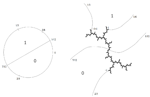
Figure 1. Left: the kneading sequence of an external angle $\vartheta$ (here $\vartheta=1/6$) is defined as the itinerary of the orbit of $\vartheta$ under angle doubling, taken with respect to the partition formed by the angles $\vartheta/2$ and $(\vartheta+1)/2$. Right: in the dynamics of a polynomial for which the $\vartheta$-ray lands at the critical value, an analogous partition is formed by the dynamic rays at angles $\vartheta/2$ and $(\vartheta+1)/2$, which land together at the critical point.

Note that in the definition of the kneading sequence, a change in $\vartheta$ amounts to a change in the orbit $\mbox{\rm orb}_{D}(\vartheta)$, as well as a change in the partition itself. Our definition involves the convention that every kneading sequence $\nu(\vartheta)$ starts with the symbol ${\tt 1}$, except for $\vartheta=0$.

A kneading sequence $\nu$ contains a ${\tt\star}$ at position $n$ if and only if $\vartheta$ is periodic with period $n$; the exact period of $\vartheta$ may divide $n$. (There are also non-periodic angles that yield periodic kneading sequences without ${\tt\star}$.) We say that a sequence $\nu$ is ${\tt\star}$-periodic of period $n$ if $\nu=\overline{\nu_{1}\ldots\nu_{n-1}{\tt\star}}$ with $\nu_{1}={\tt 1}$ and $\nu_{i}\in\{{\tt 0},{\tt 1}\}$ for $1<i<n$; this happens if and only if $\vartheta$ is periodic of exact period $n$. Write $\mathbb{N}=\{0,1,2,3,\dots\}$ and ${\mathbb{N}^{*}}=\{1,2,3,\dots\}$. Let

$$\Sigma := \{{\tt 0},{\tt 1}\}^{\mathbb{N}^{*}}\,\,,$$

$$\Sigma^{1} := \{\nu\in\Sigma\colon\mbox{the first entry in $\nu$ is ${\tt 1}$}\}\,\,,$$

$$\Sigma^{\star} := \Sigma^{1}\cup\{\mbox{all ${\tt\star}$-periodic sequences except $\overline{{\tt\star}}$}\}\,\,.$$

The metric on $\Sigma$ is $d(x,y)=\sum_{i=1}^{\infty}2^{-i}|x_{i}-y_{i}|$. In order to avoid silly counterexamples, $\overline{{\tt\star}}$ is not considered to belong to $\Sigma^{\star}$. All sequences in $\Sigma^{\star}$ will be called kneading sequences, regardless of whether or not they occur as the image of an angle $\vartheta\in{\mathbb{S}}^{1}$.

To compress the information of the kneading sequence $\nu$, it is useful to introduce the $\rho$-function.

Definition 2.2.

($\rho$-Function and Internal Address).

For a sequence $\nu\in\Sigma^{\star}$, define

$$\rho_{\nu}:{\mathbb{N}^{*}}\to{\mathbb{N}^{*}}\cup\{\infty\},\quad\rho_{\nu}(n)=\inf\{k>n:\nu_{k}\neq\nu_{k-n}\}.$$

We usually write $\rho$ for $\rho_{\nu}$ and call $\mbox{\rm orb}_{\rho}(k)=\{\rho^{\circ i}(k)\}_{i\geq 0}$ the $\rho$-orbit of $k$. The case $k=1$ is the most important one; this is the internal address of $\nu$ and we denote it as

$$1=S_{0}\to S_{1}\to S_{2}\to\dots$$

The name internal address is motivated by the fact that if $\vartheta$ is the parameter angle of $c\in\partial\mathcal{M}$ and $\gamma\subset\mathcal{M}$ is a (combinatorial) arc connecting $0$ to $c$, then the periods of the hyperbolic components of $\mathcal{M}$ intersecting $\gamma$ having a lower period than any later hyperbolic component intersecting $\gamma$ form precisely the entries of the internal address, see [LS, Sch1].

The map from kneading sequences in $\Sigma^{1}$ to internal addresses is injective. In fact, the algorithm of this map can easily be inverted:

Algorithm 2.3.

(From Internal Address to Kneading Sequence).

The following inductive algorithm turns internal addresses into kneading sequences in $\Sigma^{1}$: the internal address $S_{0}=1$ has kneading sequence $\overline{{\tt 1}}$, and given the kneading sequence $\nu^{k}$ associated to $1\to S_{1}\to\ldots\to S_{k}$, the kneading sequence associated to $1\to S_{1}\to\ldots\to S_{k}\to S_{k+1}$ consists of the first $S_{k+1}-1$ entries of $\nu^{k}$, followed by the opposite to the entry $S_{k+1}$ in $\nu$ (switching ${\tt 0}$ and ${\tt 1}$), and then repeating these $S_{k+1}$ entries periodically.

Proof.

The kneading sequence $\overline{{\tt 1}}$ has internal address $1$. If $\nu^{k}$ has internal address $1\to S_{1}\ldots\to S_{k}$ and $\nu$ is the kneading sequence of period $S_{k+1}$ as constructed in the algorithm, then the internal address of $\nu$ clearly starts with $1\to S_{1}\to\ldots\to S_{k}$, and $\rho_{\nu}(S_{k})=S_{k+1}$, so the internal address of $\nu$ is $1\to S_{1}\to\ldots\to S_{k}\to S_{k+1}$. $\Box$

2.3. Hausdorff Dimension of Biaccessible Angles

Our results are about biaccessible points both in Julia sets and in the Mandelbrot set. If $K\subset\mathbb{C}$ is compact, then a point $z\in\partial K$ is topologically biaccessible if there are two curves $\gamma_{1},\gamma_{2}\colon[0,1]\to\overline{\mathbb{C}}$ with $\gamma_{i}(0)=\infty$, $\gamma_{i}(1)=z$, $\gamma_{i}([0,1))\subset\overline{\mathbb{C}}\setminus K$ (for $i=1,2$) and so that $\gamma_{1}$ and $\gamma_{2}$ are not homotopic in $\overline{\mathbb{C}}\setminus K$ fixing endpoints. We will translate this into a combinatorial setting in Section 3 but first state our main results here. These results will be given in terms of two quantities $N$ and $\kappa$ that we define first.

(i) For a kneading sequence $\nu={\tt 1}\nu_{2}\nu_{3}\nu_{4}\dots\in\Sigma^{1}$, let

(2.1) $$N=N(\nu):=1+\min\{i>1\colon\nu_{i}={\tt 1}\},$$

so that $N(\nu)-1$ is the position of the second ${\tt 1}$ in $\nu$ (and $N(\nu)=\infty$ if $\nu={\tt 1}\overline{{\tt 0}}$); hence $N(\nu)\geq 3$. Set $M:=\lfloor N/2\rfloor-1$ and

(2.2) $$U_{1}(N) :=1-\frac{1}{2^{N}\log 2^{N}}\qquad\text{and}$$

(2.6) $$L_{1}(N) :=\left\{\begin{array}[]{ll}1-\frac{1}{2^{M}\log 2^{M}}&\text{ if }N\geq 6\\ 1/2&\text{ if }N=5,\\ 0&\text{ if }N\in\{3,4\}.\end{array}\right.$$

Finally, set $L_{1}(N)=U_{1}(N)=1$ if $N=\infty$.

(ii) For a kneading sequence $\nu$ with internal address $1\to S_{1}\to S_{2}\to\dots$, let

(2.7) $$\kappa=\kappa(\nu):=\sup\{k\geq 1:S_{j}\text{ is a multiple of }S_{j-1}\text{ for all }1\leq j\leq k\}\;.$$

We define $L_{2}(S_{\kappa})$ and $U_{2}(S_{\kappa})$ as follows:

• if $\kappa=\infty$, then $L_{2}(S_{\kappa})=U_{2}(S_{\kappa})=0$;

• if $\kappa<\infty$ and $\nu$ is periodic of period $S_{\kappa}$, then again $L_{2}(S_{\kappa})=U_{2}(S_{\kappa})=0$;

• otherwise (i.e., if $\kappa<\infty$ and $\nu$ is not periodic of period $S_{\kappa}$, hence $S_{\kappa+1}<\infty$), we set

  (2.8) $$L_{2}(S_{\kappa}):={1}/{S_{\kappa+1}},\quad U_{2}(S_{\kappa}):=\sqrt{{7}/{S_{\kappa+1}}}\;.$$

With these definitions, define the interval

(2.9) $${\mathcal{I}}(N,S):=\left[\ \max\left\{L_{1}(N),L_{2}(S)\rule{0.0pt}{10.0pt}\right\}\ ,\ \min\left\{U_{1}(N),U_{2}(S)\rule{0.0pt}{10.0pt}\right\}\ \rule{0.0pt}{12.0pt}\right].$$

We define combinatorial biaccessibility in Definition 3.3; this leads to the following two sets (for the dynamical planes respectively parameter space) that we will investigate:

$${\mathcal{B}iac}_{\vartheta}=\{\varphi\in{\mathbb{S}}^{1}\colon\text{$\varphi$ is combinatorially biaccessible with respect to $\vartheta$}\},$$

and

$${\mathcal{B}iac}=\{\vartheta\in{\mathbb{S}}^{1}\colon\text{$\vartheta$ is combinatorially biaccessible}\}.$$

With these definitions, our first main result is as follows.

Theorem 2.4.

(Hausdorff Dimension of Biaccessible Angles).

For every parameter angle $\vartheta\in{\mathbb{S}}^{1}$,

$$\dim_{H}({\mathcal{B}iac}_{\vartheta})\in{\mathcal{I}}(N,S)$$

for $N=N(\nu(\vartheta))$ and $S=S_{\kappa}(\nu(\vartheta))$. In particular, the set of biaccessible external dynamic angles has Hausdorff dimension less than $1$ unless $\vartheta=1/2$.

This implies that the harmonic measure of the biaccessible points in quadratic Julia sets is zero, unless $\vartheta=\frac{1}{2}$; this was of course known earlier [Sm, Za, Zd]. Our result that the Hausdorff dimension of biaccessible angles is less than $1$ except when the Julia set is an interval (which, in the quadratic case, means $\vartheta=1/2$) was later generalized to all degrees in [MS].

The similarity of Theorem 2.4 and the next one underlines the similarity of the structure of $\mathcal{J}_{c}$ and the local structure of $\mathcal{M}$ near $c$ as in [Ta1].

Theorem 2.5.

(Hausdorff Dimension of Biaccessible Parameter Angles).

For any $N\geq 3,\kappa\geq 1$ we have

$$\dim_{H}\left({\mathcal{B}iac}\cap\left\{\vartheta\in{\mathbb{S}}^{1}:N(\nu(\vartheta))=N\text{ and }S_{\kappa}(\nu(\vartheta))=S\right\}\right)\in{\mathcal{I}}(N,\kappa).$$

Remark 2.6.

The estimate $[L_{2}(S_{\kappa}),U_{2}(S_{\kappa})]$ is best where the biaccessibility dimension is small. In every case we either have $L_{2}(S_{\kappa})=U_{2}(S_{\kappa})=0$ or $U_{2}(S_{\kappa})>L_{2}(S_{\kappa})>0$, so that we specify exactly in which situation the biaccessibility dimension is zero: this happens if and only if the parameter is on the closed main molecule (see Proposition 2.11). Our result implies continuity of the biaccessibility dimension on the closed main molecule of $\mathcal{M}$: if $(c_{n})$ is a sequence of parameters in $\mathcal{M}$ that converges to the main molecule and with associated external angles $\vartheta_{n}$, then $\dim_{H}({\mathcal{B}iac}_{\vartheta_{n}})\to 0$.

Similarly, the estimate $[L_{1}(N),U_{1}(N)]$ is especially good near parameters where the biaccessibility dimension is maximal, that is near the “antenna tip” at $c=-2$. Again, we have $L_{1}(N)=U_{1}(N)=1$ or $L_{1}(N)<U_{1}(N)<1$, so we specify exactly in which situation the dimension is $1$: this happens if and only if $c=-2$, which was generalized in [MS]. Again our result implies continuity in the approach to this point.

Remark 2.7.

Since, as mentioned before, core entropy (appropriately defined for all polynomials in $\mathcal{M}$) equals biaccessibility dimension times by $\log 2$, these results give a different proof for continuity of the core entropy at the main molecule and at $c=-2$ (i.e., for parameters with core entropy in $\{0,\log 2\}$) with precise estimates. (Of course, continuity everywhere was proved in [Ti2, DS].)

Remark 2.8.

In particular, the set of biaccessible parameter angles has Hausdorff dimension $1$ but Lebesgue measure zero: outside of every neighborhood of $\frac{1}{2}$ they have Hausdorff dimension less than $1$. The same holds for the set of parameter angles with landing point on the real antenna $\mathcal{M}\cap\mathbb{R}$. This follows because the collection of kneading sequences $\nu$ of the form used in our proof (formula (6.1) to be precise) has the property that $\mbox{\rm orb}_{\rho}(1)\cap\mbox{\rm orb}_{\rho}(N-1)=\emptyset$. According to [Thn], this means that $\nu$ is the kneading sequence of a real quadratic map, so the part of the proof below that refers to (6.1) (i.e., biaccessible parameter angles close to $\frac{1}{2}$) automatically gives that set of “real” parameter angles has indeed Hausdorff dimension $1$. We would also like to mention recent work by Tiozzo especially on the kneading sequences and external angles on $\mathcal{M}\cap\mathbb{R}$ [Ti1]: for every $c\in\mathcal{M}\cap\mathbb{R}$, the set of external angles of $\mathcal{M}$ that lands on $[c,0]\subset(\mathcal{M}\cap\mathbb{R})$ has the same Hausdorff dimension as the set of all biaccessible angles of $\mathcal{J}_{c}$.

2.4. Renormalizable Angles

Now we draw some direct consequences of the methods of the main results that have to do with renormalization.

Definition 2.9.

(Renormalizable).

A quadratic polynomial $p_{c}:z\mapsto z^{2}+c$ is $M$-renormalizable for $M\geq 2$ if there exist neighborhoods $U\subset V$ of the critical point $0$, with $U$ compactly contained in $V$, such that $p_{c}^{\circ M}:U\to V$ is a degree $2$ branched covering such that $p_{c}^{\circ iM}(0)\in U$ for all $i\geq 1$. The integer $M$ is called the period of renormalization. The set $K_{U}:=\{z\in U\colon p_{c}^{\circ Mi}(z)\in U\text{ for all }i\geq 0\}$ is called the little filled-in Julia set of the renormalization. The renormalization is called simple if $K_{U}\cap p_{c}^{\circ i}(K_{U})$ does not disconnect $K_{U}$ for $i=1,\dots,M-1$; otherwise it is called a crossed renormalization.

If $p_{c}$ is simple renormalizable of period $M$, then $M=S_{k}$ is an entry in the internal address and all successive entries $S_{j}$, $j\geq k$, are multiples of $M$, and conversely [LS, Sch1]. The corresponding kneading sequence has the form

(2.10) $$\nu=\nu(\vartheta)=\nu_{1}\nu_{2}\dots\nu_{M-1}\nu_{M}\nu_{1}\nu_{2}\dots\nu_{M-1}\nu_{2M}\nu_{1}\nu_{2}\dots\nu_{M-1}\nu_{3M}\dots$$

where either $\nu_{M}\nu_{2M}\nu_{3M}\dots$ or its opposite sequence $\nu^{\prime}_{M}\nu^{\prime}_{2M}\nu^{\prime}_{3M}\dots$ (where $\nu^{\prime}_{i}={\tt 1}-\nu_{i}$) is the kneading sequence of the renormalization $p_{c}^{\circ M}$.

We recover a result by Manning on external angles [Man, page 523] and extend it to kneading sequences as follows.

Proposition 2.10.

(Dimension of Renormalizable Angles and Kneading Sequences).

For any $M\geq 2$, the Hausdorff dimension of the set of simple $M$-renormalizable parameter angles as well as of the set of simple $M$-renormalizable kneading sequences is at most $1/M$. The Hausdorff dimension of infinitely renormalizable parameter angles as well as of infinitely renormalizable kneading sequences is $0$.

Let some angle $\vartheta$ have internal address $1\to S_{1}\to S_{2}\to\dots$ or $1\to S_{1}\to S_{2}\to\dots\to S_{k}$ (if it is finite). If $S_{j}$ is a multiple of $S_{j-1}$ for all $1\leq j<\infty$ (or $1\leq j\leq k$), then we say that $\vartheta$ is associated to the main molecule of the Mandelbrot set. The angle may be non-renormalizable (if the internal address is just the single entry $1$), finitely renormalizable (if the internal address has finitely many entries, but at least $2$), or infinitely renormalizable (if the internal address is infinite).

The best known example of an infinitely renormalizable map from the main molecule is the Feigenbaum-Coullet-Tresser map $p_{c}$ with $c=-1.4011551890...$, where $S_{j}=2^{j}$.

Proposition 2.11.

(Main Molecule Angles).

The following two conditions are equivalent for a parameter angle $\vartheta$:

• $\dim_{H}({\mathcal{B}iac}_{\vartheta})=0$;

• $\vartheta$ is associated to the main molecule of $\mathcal{M}$.

3. The Combinatorial Approach

3.1. The Hubbard Tree and non-admissible kneading sequences

The Hubbard tree of a postcritically finite polynomial is defined as the connected hull of the union of all critical orbits within the filled-in Julia set (subject to a regularity condition on how to pass through bounded Fatou components). We view a Hubbard tree of a quadratic polynomial as a finite abstract tree $T$ with dynamics $f\colon T\to T$ subject to the following conditions:

1. $f:T\to T$ is a local embedding, except at a single critical point $c_{0}$.

2. This critical point divides $T$ into (at most) two parts, labeled ${\tt 1}$ (the part containing the critical value $c_{1}=f(c_{0})$) and ${\tt 0}$, while $c_{0}$ itself gets the symbol $\star$. Using these symbols, we can define itineraries in the usual way.

3. The endpoints of $T$ lie on the critical orbit.

4. All marked points (i.e., branch points and points on the critical orbit) have distinct itineraries (with respect to the partition introduced by $c_{0}$).

It was shown in [BKS] that for every ${\tt\star}$-periodic or preperiodic $\nu$, there is a Hubbard tree $(T,f)$ such that $\nu$ is the itinerary of the critical value. Moreover, $\nu$ uniquely determines the dynamics on the marked points, and their numbers of arms, so the pair $(T,f)$ is determined uniquely as an abstract tree with dynamics (up to homotopy relative to the marked points). However, there can be multiple ways (up to homotopy) of embedding $T$ into $\mathbb{C}$ such that the dynamics $f$ extends to local homeomorphism on $\mathbb{C}$. This depends on how the arms of a branch point $p$ are arranged; if $p$ is periodic of period $n$, then $f^{\circ n}$ permutes the arms of $p$ in a transitive way, but the choice of combinatorial rotation number is still free. This is the reason why multiple parameter angles lead to the same kneading sequence (see also Figure 2) and the same internal address. In order to distinguish different embeddings of these trees, angled internal addresses are required [Sch1]. We will come back to this in Section 7, where we estimate the total number of different embeddings in $\mathbb{C}$.

Not every sequence in $\Sigma^{1}$ or $\Sigma^{\star}$ occurs as the kneading sequence of an external angle, or of a quadratic polynomial, not even every periodic sequence. The main result of [BrS] is an explicit condition that states which sequences occur: a kneading sequence or internal address does occur unless it fails the following admissibility condition for some period $m$. Failing the condition forces the Hubbard tree to have a periodic branch point of period $m$ with certain specific properties; such periodic orbits are called evil.

Definition 3.1.

(The Admissibility Condition).

A kneading sequence $\nu\in\Sigma^{\star}$ fails the admissibility condition for period $m$ (the evil period) if the following three conditions hold:

1. the internal address of $\nu$ does not contain $m$;

2. if $k<m$ divides $m$, then $\rho(k)\leq m$;

3. $\rho(m)<\infty$ and if $r\in\{1,\ldots,m\}$ is congruent to $\rho(m)$ modulo $m$, then $\mbox{\rm orb}_{\rho}(r)$ contains $m$.

A kneading sequence fails the admissibility condition if it does so for some $m\geq 1$.

An internal address fails the admissibility condition if its associated kneading sequence (from Definition 1 and Algorithm 2.3) does.

Remark 3.2.

The main result in [BKS] is that for every ${\tt\star}$-periodic kneading sequence $\nu$ there exists a unique Hubbard tree (without embedding into $\mathbb{C}$) for which the critical value has kneading sequence $\nu$ (with respect to the unique critical point of this tree), and the main result of [BrS] is that this tree can be embedded into the plane so that the dynamics is compatible with this embedding if and only if $\nu$ does not fail this admissibility condition. Since every tree thus embedded is realized by a quadratic polynomial and has two characteristic periodic dynamic rays, this means that a ${\tt\star}$-periodic kneading sequence is realized by an external angle if and only if the kneading sequence does not fail the admissibility condition.

3.2. Combinatorial biaccessibility

In this section we give the central combinatorial characterization of biaccessibility. We denote an ordered pair of angles by $\langle\varphi,\varphi^{\prime}\rangle$ (this is technically the same as the more usual notation $(\varphi,\varphi^{\prime})$ for an element of ${\mathbb{S}}^{1}\times{\mathbb{S}}^{1}$, but we will reserve the latter for the open interval). We say that an angle pair $\langle\varphi,\varphi^{\prime}\rangle$ separates another angle pair $\langle\tilde{\varphi},\tilde{\varphi}^{\prime}\rangle$ if $\tilde{\varphi}$ and $\tilde{\varphi}^{\prime}$ are in different components of ${\mathbb{S}}^{1}\setminus\{\varphi,\varphi^{\prime}\}$.

Suppose that in some dynamical plane the dynamic ray at angle $\vartheta$ lands at the critical value (a discussion that holds in more general situations can be given in terms of Thurston laminations as defined in [Th1]). Then the two rays at angles $\vartheta/2$ and $(1+\vartheta)/2$ land at the critical point, so the critical point is biaccessible and the two angles $\vartheta/2$ and $(1+\vartheta)/2$ are biaccessible angles (with respect to the angle $\vartheta$). We say that $\langle\vartheta/2,(1+\vartheta)/2\rangle$ forms the critical angle pair (compare Figure 1). Similarly, all further angles on the backwards orbit of $\vartheta$ are biaccessible angles. By induction on $k$ (the number of iterations required to reach $\vartheta$), each angle $\varphi$ on the backwards orbit of $\vartheta$ has a unique angle $\varphi^{\prime}\neq\varphi$ on the backwards orbit of $\vartheta$ with $\mbox{{\sc Step}}(\varphi)=\mbox{{\sc Step}}(\varphi^{\prime})$ that is not separated by precritical angle pairs with lower values of Step, and then $\langle\varphi,\varphi^{\prime}\rangle$ forms a precritical angle pair. In particular, all precritical points are biaccessible, which forms a countable set. Therefore, to find the Hausdorff dimension of biaccessible angles in the dynamics modeled by the external angle $\vartheta$, we only need to investigate angles $\varphi$ that are not on the backwards orbit of $\vartheta$, or equivalently we only need to investigate itineraries in $\Sigma=\{{\tt 0},{\tt 1}\}^{\mathbb{N}^{*}}$.

In parameter space, it is known that all parameter rays at periodic angles of fixed period $n>1$ land in pairs [DH, Mi2, Sch4], so their landing points are biaccessible and all periodic angles are biaccessible angles in parameter space. If two parameter rays at periodic angles $\vartheta_{1}$ and $\vartheta_{2}$ (necessarily of equal period) land together, we say that $\langle\vartheta_{1},\vartheta_{2}\rangle$ forms a periodic parameter angle pair. Since all periodic external angles are thus biaccessible (in parameter space, at least when the period is $2$ or greater), and these are exactly the angles with ${\tt\star}$-periodic kneading sequences and they form a countable set, it follows that the Hausdorff dimension of biaccessible angles in parameter space is determined by angles with kneading sequences in $\Sigma$, and periodic parameter angle pairs give a necessary condition, and this condition turns out to be sufficient except for sets of dimension zero).

We can now give a combinatorial definition of biaccessibility, both in the dynamical plane and in parameter space.

Definition 3.3.

(Combinatorial Biaccessibility and Angle Pairs).

An angle $\varphi\in{\mathbb{S}}^{1}$ is called combinatorially biaccessible with respect to $\vartheta\in{\mathbb{S}}^{1}$ if there is a $\varphi^{\prime}\in{\mathbb{S}}^{1}$ with $\varphi^{\prime}\neq\varphi$ such that no precritical angle pair separates $\varphi$ from $\varphi^{\prime}$. We call $\langle\varphi,\varphi^{\prime}\rangle$ a dynamic angle pair.

An angle $\vartheta\in{\mathbb{S}}^{1}$ with non-periodic kneading sequence in $\Sigma$ is called combinatorially biaccessible (in parameter space) if there is a $\vartheta^{\prime}\in{\mathbb{S}}^{1}$ with $\vartheta^{\prime}\neq\vartheta$ so that no periodic parameter angle pair $\langle\vartheta_{1},\vartheta_{2}\rangle$ separates $\vartheta$ from $\vartheta^{\prime}$. We call $\langle\vartheta,\vartheta^{\prime}\rangle$ a parameter angle pair.

Remark 3.4.

All precritical angles are combinatorially biaccessible according to this definition. Indeed, if $\vartheta$ is not combinatorially biaccessible, then $\langle\vartheta/2,(\vartheta+1)/2\rangle$ is an dynamic angle pair that is not separated by any other precritical angle pair, and this carries over to preimage angle pairs of $\langle\vartheta/2,(\vartheta+1)/2\rangle$. If, on the other hand, $\vartheta$ is combinatorially biaccessible, say $\langle\vartheta,\vartheta^{\prime}\rangle$ forms the corresponding dynamic angle pair, then $\langle\vartheta/2,\vartheta^{\prime}/2\rangle$ and $\langle(\vartheta+1)/2,(\vartheta^{\prime}+1)/2\rangle$ are angle pairs that are not separated by precritical angle pairs. It is thus not relevant that $\langle\vartheta/2,(\vartheta+1)/2\rangle$ and $\langle\vartheta^{\prime}/2,(\vartheta^{\prime}+1)/2\rangle$ separate each other (while landing at the same point).

Our combinatorial estimates will all be with respect to this definition (in dynamical planes and in parameter space). In order to explain how this definition relates to the topological concept of biaccessibility as introduced earlier, we start with a simple lemma.

Lemma 3.5.

(Combinatorially Biaccessible Angle Pairs).

An angle $\varphi$ is combinatorially biaccessible with respect to $\vartheta$ if and only if there is a $\varphi^{\prime}\in{\mathbb{S}}^{1}$ with $\varphi^{\prime}\neq\varphi$ so that $\nu_{\vartheta}(\varphi)=\nu_{\vartheta}(\varphi^{\prime})$.

Proof.

If two angles $\varphi\neq\varphi^{\prime}$ are separated by precritical angle pairs, then the angle pair with lowest value of Step is always unique (because two angle pairs with equal value of Step are always separated by an angle pair with lower value, which is easily confirmed inductively).

If two angles $\varphi\neq\varphi^{\prime}$ are separated by a unique precritical angle pair $\langle\vartheta_{1},\vartheta_{2}\rangle$ with $\mbox{{\sc Step}}(\vartheta_{1})=\mbox{{\sc Step}}(\vartheta_{2})=k$, then $\nu_{\vartheta}(\varphi)$ and $\nu_{\vartheta}(\varphi^{\prime})$ differ in the $k$-th position.

Conversely, if the $k$-th entries of $\nu_{\vartheta}(\varphi)$ and $\nu_{\vartheta}(\varphi^{\prime})$ are different, then $D^{\circ(k-1)}(\varphi)$ and $D^{\circ(k-1)}(\varphi^{\prime})$ are separated by the diameter $\langle\vartheta/2,(1+\vartheta)/2\rangle$, and by taking $k-1$ preimages it follows that $\varphi$ and $\varphi^{\prime}$ are separated by a precritical angle pair $\langle\vartheta_{1},\vartheta_{2}\rangle$ with $\mbox{{\sc Step}}(\vartheta_{1})=\mbox{{\sc Step}}(\vartheta_{2})=k$. $\Box$

The corresponding statement in parameter space will be discussed below.

3.3. Combinatorial and topological biaccessibility

We will now relate combinatorial biaccessibility with respect to $\vartheta$ to topological biaccessibility in a Julia set for which the dynamic ray at angle $\vartheta$ lands at the critical value.

Proposition 3.6.

(Topologically and Combinatorially Biaccessible Angles).

For every quadratic polynomial with connected Julia set, the set of topologically biaccessible angles is a subset of the set of combinatorially biaccessible angles. In every case, these two sets have the same Hausdorff dimension.

Proof.

If two rays at angles $\varphi$ and $\varphi^{\prime}$ land together at a point that is not on the backwards orbit of the critical point, then $\varphi$ and $\varphi^{\prime}$ clearly cannot be separated by a precritical angle pair. Therefore, combinatorial biaccessibility in the sense of Definition 3.3 is necessary for topological biaccessibility in a dynamical plane.

The converse is true at least in locally connected Julia sets; however, some care is necessary because local connectivity in itself does not seem to imply easily that combinatorially biaccessible angle pairs actually have rays that land at a common point. However, the somewhat stronger property of trivial fibers is sufficient, see [Sch2, Sch5]: by definition, a point $z$ within a Julia set $\mathcal{J}$ has trivial fiber if, for every $z^{\prime}\in\mathcal{J}\setminus\{z\}$, there is a pair of dynamic rays at periodic angles that separates $z^{\prime}$ from $z$. This implies local connectivity of $\mathcal{J}$ at $z$, but it is locally a strictly stronger property. In particular, it implies that every $z^{\prime}\in\mathcal{J}\setminus\{z\}$ can also be separated from $z$ by a pair of rays that land at the same precritical point. Hence, if all fibers are trivial, then every angle $\varphi$ that is combinatorially biaccessible is in fact topologically biaccessible: there is another angle $\varphi^{\prime}$ so that the rays at angles $\varphi$ and $\varphi^{\prime}$ land together. (Note that in the case of bounded Fatou components, a slight modification is necessary in the definition of fibers, allowing for separation lines to pass through bounded Fatou components [Sch2].)

In fact, all currently known proofs of local connectivity of Julia sets of quadratic polynomials show that all fibers are trivial: this is true for polynomials with attracting or parabolic periodic orbits (Douady and Hubbard [DH]), as well as for all quadratic polynomials for which all periodic orbits are repelling and that are not infinitely renormalizable (Yoccoz [HY]; for the renormalizable case see also [Sch3]), and for various infinitely renormalizable quadratics in work of Kahn and Lyubich (see [Ly1, KL1, KL2] and the references therein), and finally in the case of a Siegel disk of bounded type [Pet]. A separate argument is the general result that if a polynomial Julia set is locally connected at every point, then all fibers are trivial [Sch3] (as mentioned, this implication is not true at individual points $z$).

The relation between combinatorial and topological biaccessibility may thus be non-trivial only in the presence of irrationally indifferent cycles or for infinitely renormalizable polynomials. In fact, for a quadratic polynomial with an indifferent cycle of period $1$, the set of angles that is not separated from the indifferent fixed point by a precritical angle pair has Hausdorff dimension zero [BuS] (this is the set of external angles of the Siegel disk in case the Julia set is locally connected). All other angles cannot be part of a biaccessible angle pair [SZ], so biaccessibility concerns only a set of Hausdorff dimension zero (including the backwards orbit of all rays that are not separated from the indifferent fixed point, which is a countable union), so this does not affect our dimension estimates.

If there is an indifferent periodic cycle of period $M>1$, then the set of external angles related to this cycle still has dimension zero, and all other points have trivial fibers [HY, Sch3], so combinatorially and topologically biaccessible angles coincide.

Finally, for infinitely renormalizable polynomials (see Definition 2.9), we note first that, for the same reason as before, all points $z\in\mathcal{J}$ that are outside of the little $M$-renormalizable Julia set for some $M$ have trivial fibers, while external angles corresponding to $M$-renormalization are in a set of Hausdorff dimension at most $1/M$ (see Section 8). Therefore, if a polynomial is infinitely renormalizable, then all angles belong to trivial fibers with the exception of a set of dimension zero, which again does not affect our estimates. $\Box$

Proposition 3.7.

(Topologically and Combinatorially Biaccessible Angles in $\mathcal{M}$).

For the Mandelbrot set, the set of topologically biaccessible angles is a subset of the set of combinatorially biaccessible angles, and both sets have the same Hausdorff dimension.

Proof.

If two parameter rays land together, then they cannot be separated by a parameter ray-pair at periodic angles (the landing point of the latter is not the landing point of any parameter ray except the two periodic ones). This implies that an angle can only be topologically biaccessible if it is combinatorially biaccessible in the sense of Definition 3.3.

We will now argue that “most” combinatorially biaccessible angles are topologically biaccessible (except possibly for a set of dimension zero). Of course, the set of external angles that do not land has always Hausdorff dimension zero, but this is not a sufficient argument: we also need to consider those rays that land, but possibly not at the same point as another ray at a combinatorially associated angle.

The set of angles in parameter space that are associated to $M$-renormalizable parameters has again Hausdorff dimension at most $1/M$ (again Section 8), so the set of angles that are associated to infinitely renormalizable parameters has dimension zero and does not affect our estimates. Similarly, the set of angles that are associated to any particular hyperbolic component have Hausdorff dimension zero, see Corollary 7.5.

Therefore, except for a set of angles of Hausdorff dimension zero, every parameter ray is associated to a fiber of $\mathcal{M}$ corresponding to polynomials for which all cycles are repelling and which are not infinitely renormalizable, and such fibers are trivial by [HY]. Fibers of $\mathcal{M}$ are defined in terms of parameter ray-pairs at periodic angles, so if two parameter rays are not separated by parameter ray-pairs of periodic angles (and are not in the exceptional set), then they belong at the same fiber and thus land at the same point; so for all angles except for a set of dimension zero, combinatorial biaccessibility implies topological biaccessibility. $\Box$

Remark 3.8.

In parameter space, it may be worth noting that parameter rays at periodic angles (which have ${\tt\star}$-periodic kneading sequences) always land in pairs and are thus topologically biaccessible. Moreover, there are uncountably many further parameter rays that accumulate at hyperbolic components: their external angles have periodic (but not ${\tt\star}$-periodic) kneading sequences, and these rays land at a boundary point of a hyperbolic component (with irrationally indifferent dynamics). These rays are all not separated by periodic parameter ray-pairs and thus combinatorially biaccessible, but they are the only rays landing at the same point, so they are not topologically biaccessible. These angles (from a zero-dimensional set, see Corollary 7.5) thus form a difference between the two definitions of biaccessibility. A more precise definition of combinatorial biaccessibility would thus be “an angle $\varphi$ is combinatorially biaccessible if either there is an angle $\varphi^{\prime}$ so that $\varphi$ and $\varphi^{\prime}$ are not separated by a periodic angle pair, or if the kneading sequence $\nu(\varphi)$ is periodic but not ${\tt\star}$-periodic”. This definition would be more cumbersome without strengthening Proposition 3.7 — however, if all fibers of $\mathcal{M}$ were trivial (which is equivalent to local connectivity of $\mathcal{M}$ [Sch5]), then topological and combinatorial biaccessibility of $\mathcal{M}$ in this sense would coincide.

Definition 3.3 is thus a good combinatorial description of biaccessibility, ignoring topological subtleties.

3.4. Combinatorial biaccessibility, itineraries, and kneading sequences

In order to investigate biaccessibility from a combinatorial point of view, we translate it to the setting of itineraries. In order to do this, we extend the definition of the $\rho$-function to itineraries.

For a kneading sequence $\nu\in\Sigma^{\star}$ and $x=\nu_{\vartheta}(\varphi)\in\Sigma$, let

$$\rho_{\nu,x}(n):=\min\{k>n\colon x_{k}\neq\nu_{k-n}\}.$$

Obviously, $\rho_{\nu,\nu}=\rho_{\nu}$ for $\rho_{\nu}$ as in Definition 1.

Lemma 3.9.

(Condition for Itinerary to be Biaccessible).

Let $\vartheta,\varphi\in{\mathbb{S}}^{1}$ be two arbitrary external angles, let $\nu:=\nu(\vartheta)$ be the kneading sequence of $\vartheta$ and let $x:=\nu_{\vartheta}(\varphi)$ be the itinerary of $\varphi$ with respect to $\vartheta$; assume that $x\in\Sigma$.

Then $\varphi$ is combinatorially biaccessible with respect to $\vartheta$ if and only if there is a $k\geq 2$ that satisfies

$$\mbox{\rm orb}_{\rho_{\nu,x}}(1)\cap\mbox{\rm orb}_{\rho_{\nu,x}}(k)=\emptyset.$$

Proof.

We use symbolic dynamics modeled after the situation that the critical value is the landing point of the ray at angle $\vartheta$. Then $\langle\vartheta/2,(1+\vartheta)/2\rangle$ is the critical angle pair with $\mbox{{\sc Step}}=1$, and all other precritical angle pairs are preimages of this one. We say that a precritical angle pair $\langle\vartheta_{k},\vartheta^{\prime}_{k}\rangle$ with $\mbox{{\sc Step}}(\vartheta_{k})=\mbox{{\sc Step}}(\vartheta^{\prime}_{k})$ is a closest precritical angle pair (to $\varphi$) if it is not separated from $\varphi$ by any precritical angle pair for which the value of Step is less than $\mbox{{\sc Step}}(\vartheta_{k})$. Since any two precritical angle pairs with equal value of Step are separated by another angle pair with lower value, for any value of Step there can be at most one closest precritical angle pair.

The closest precritical angle pair $\langle\vartheta_{1},\vartheta^{\prime}_{1}\rangle$ with $\mbox{{\sc Step}}(\vartheta_{1})=\mbox{{\sc Step}}(\vartheta^{\prime}_{n})=1$ is always $\langle\vartheta/2,(1+\vartheta)/2\rangle$. Now define a sequence $(m_{j})$ with $m_{1}=1$ and, if $\langle\vartheta_{j},\vartheta^{\prime}_{j}\rangle$ is a closest precritical angle pair with $\mbox{{\sc Step}}(\vartheta_{j})=\mbox{{\sc Step}}(\vartheta^{\prime}_{j})=m_{j}$, then let $\langle\vartheta_{j+1},\vartheta^{\prime}_{j+1}\rangle$ be the precritical angle pair with lowest value of Step that separates $\varphi$ from $\langle\vartheta_{j},\vartheta^{\prime}_{j}\rangle$; we define $m_{j+1}:=\mbox{{\sc Step}}(\vartheta_{j+1})=\mbox{{\sc Step}}(\vartheta^{\prime}_{j+1})$.

This $\rho$-itinerary describes the itinerary of $\vartheta_{j}$ and of $\vartheta^{\prime}_{j}$ (which is the same) completely: the first $m_{j}-1$ entries coincide with that of $\varphi$, i.e., with $\nu_{\vartheta}(\varphi)$, then comes a $\star$, and then the itinerary of $\vartheta$ (which is $\nu(\vartheta)$). This means $\rho_{\nu,x}(m_{j})=m_{j+1}$ for all $j$, so $(m_{j})=\mbox{\rm orb}_{\rho_{\nu},x}(1)$ (equality of sequences).

Now suppose $\langle\varphi,\varphi^{\prime}\rangle$ is a biaccessible angle pair; by definition, this means that no closest precritical angle pair $\langle\vartheta_{j},\vartheta^{\prime}_{j}\rangle$ separates $\varphi$ from $\varphi^{\prime}$, so they all (for $j>1$) separate both $\varphi$ and $\varphi^{\prime}$ from the angle pair $\langle\vartheta/2,(1+\vartheta)/2\rangle$.

Without loss of generality, we may assume that $0<\varphi<\varphi^{\prime}<1$. Then there is a precritical angle $\psi_{1}\in(\varphi,\varphi^{\prime})$ and hence a precritical angle pair $\langle\psi_{1},\psi^{\prime}_{1}\rangle\subset(\varphi,\varphi^{\prime})$; set $k_{1}:=\mbox{{\sc Step}}(\psi_{1})=\mbox{{\sc Step}}(\psi_{2})$.

As before, for a precritical angle pair $\langle\psi_{j},\psi^{\prime}_{j}\rangle$, define a sequence $k_{j}$ so that $\langle\psi_{j+1},\psi^{\prime}_{j+1}\rangle$ is the precritical angle pair with lowest value of Step that separates $\varphi$ from $\langle\psi_{j},\psi_{j+1}\rangle$; we define $k_{j+1}:=\mbox{{\sc Step}}(\psi_{j+1})=\mbox{{\sc Step}}(\psi^{\prime}_{j+1})$. Then all $\{{\psi_{j}},{\psi^{\prime}_{j}}\}\subset(\varphi,\varphi^{\prime})$, so none of the $\langle\psi_{j},\psi^{\prime}_{j}\rangle$ separate $\langle\varphi,\varphi^{\prime}\rangle$ from $\langle\vartheta_{1},\vartheta^{\prime}_{1}\rangle$. Therefore, the sequences $(m_{j})$ and $(k_{j})$ are disjoint.

Finally, comparing itineraries, it is easy to check that $(k_{j})=\mbox{\rm orb}_{\rho_{\nu,x}}(k_{1})$, and this proves the existence of two disjoint $\rho_{\nu,x}$-orbits as required.

The converse is similar: $\mbox{\rm orb}_{\rho_{\nu,x}}(1)$ always describes the sequence of closest precritical angle pairs $\langle\vartheta_{j},\vartheta^{\prime}_{j}\rangle$, starting at the diameter, that separate the previous angle pair from $\varphi$. If we label so that $\vartheta_{j}<\vartheta^{\prime}_{j}$, then the sequence $(\vartheta_{j})$ is monotonically increasing and $(\vartheta^{\prime}_{j})$ is monotonically decreasing. Denote their limits by $\vartheta_{\infty}\leq\vartheta^{\prime}_{\infty}$. Observe that if $\vartheta_{\infty}<\vartheta^{\prime}_{\infty}$, then $\langle\vartheta_{\infty},\vartheta^{\prime}_{\infty}\rangle$ forms a biaccessible angle pair. Even if $\varphi\not\in\{\vartheta_{\infty},\vartheta^{\prime}_{\infty}\}$, both $\langle\varphi,\vartheta_{\infty}\rangle$ and $\langle\varphi,\vartheta^{\prime}_{\infty}\rangle$ are biaccessible angle pairs. In order to prove that $\varphi$ is combinatorially biaccessible, it thus suffices to prove that $\vartheta_{\infty}<\vartheta^{\prime}_{\infty}$.

This is assured by the existence of $\mbox{\rm orb}_{\rho_{\nu,x}}(k)$: this describes a similar sequence starting with the closest precritical angle pair for which Step has the value $k$. If these sequences are disjoint for some $k$, then none of the associated angle pairs can be separated from $\varphi$ by any $\langle\vartheta_{j},\vartheta^{\prime}_{j}\rangle$, and every angle pair described by $\mbox{\rm orb}_{\rho_{\nu,x}}(k)$ provides a uniform lower bound for $\vartheta^{\prime}_{j}-\vartheta_{j}$, so their limits are different as required. $\Box$

Now we turn to parameter space.

Lemma 3.10.

(Biaccessible Kneading Sequence).

An angle $\vartheta$ is combinatorially biaccessible (in parameter space) in the sense of Definition 3.3 if and only if its kneading sequence $\nu=\nu(\vartheta)$ has a $k\geq 2$ such that

$$\mbox{\rm orb}_{\rho}(1)\cap\mbox{\rm orb}_{\rho}(k)=\emptyset.$$

Figure 2. Illustration of the map $\vartheta\mapsto\nu(\vartheta)$. The angles of the form $a/(2^{k}-1)$, $k\leq n$, divide ${\mathbb{S}}^{1}$ into arcs that map to components of $n$-cylinder sets.

Proof.

The structure of this proof is similar to Lemma 3.9; we use the structure given by periodic parameter angle pairs $\langle\psi,\psi^{\prime}\rangle$ of equal period that land together at a common point.

Note first that, as a function of the angle $\psi$, the $n$-th entry in the kneading sequence $\nu(\psi)$ changes between ${\tt 0}$ and ${\tt 1}$ exactly when $\psi$ is periodic of period $n$ or dividing $n$. Since angles of equal period come in pairs, it follows that if two non-periodic angles $\vartheta$ and $\vartheta^{\prime}$ are not separated by a periodic angle pair, their kneading sequences must coincide; and if the periodic ray pair of lowest period that separates them has period $n$, then the two kneading sequences differ for the first time at the $n$-th position (this statement uses the fact, known as Lavaurs’ Lemma [La], that if any two parameter angle pairs $\langle\psi_{1},\psi^{\prime}_{1}\rangle$ and $\langle\psi_{2},\psi^{\prime}_{2}\rangle$ of equal period are such that $\langle\psi_{1},\psi^{\prime}_{1}\rangle$ separates $\langle\psi_{2},\psi^{\prime}_{2}\rangle$ from the angle $0$, then the two angle pairs are separated from each other by an angle pair of lower period).

Conversely, if their kneading sequences (which must be in $\Sigma$) differ for the first time at the $n$-th position, then the lowest period of an angle pair separating $\vartheta$ and $\vartheta^{\prime}$ is exactly $n$. In particular, if the two kneading sequences coincide, then they are not separated by any periodic ray pair.

Now suppose that a non-periodic angle $\vartheta$ is combinatorially biaccessible in parameter space, i.e., there is an angle $\vartheta^{\prime}$ that is not separated from $\vartheta$ by any periodic parameter angle pair. Then $\nu(\vartheta)=\nu(\vartheta^{\prime})=:\nu$. The angle pair $\langle\vartheta_{1},\vartheta^{\prime}_{1}\rangle$ of lowest period $n_{1}$ that separates the angle $0$ from $\langle\vartheta,\vartheta^{\prime}\rangle$ must have period $n_{1}=\rho_{\nu}(1)$, and inductively the angle pair of lowest period that separates $\langle\vartheta_{j},\vartheta^{\prime}_{j}\rangle$ from $\langle\vartheta,\vartheta^{\prime}\rangle$, say $\langle\vartheta_{j+1},\vartheta^{\prime}_{j+1}\rangle$, has period $n_{j+1}=\rho_{\nu}(n_{j})$. The sequence of periods of these angle pairs is thus $\mbox{\rm orb}_{\rho_{\nu}}(1)$; this is the internal address of $\vartheta$.

Sorting the angle pairs again such that $0<\vartheta<\vartheta^{\prime}<1$ and $0<\vartheta_{j}<\vartheta^{\prime}_{j}<1$ for all $j$, it follows that the sequence $(\vartheta_{j})$ is monotonically increasing and converges to a limit in $(0,\vartheta]$, while $(\vartheta^{\prime}_{j})$ is monotonically decreasing and converges to a limit in $[\vartheta^{\prime},1)$.

Now pick a periodic angle $\psi_{1}\in(\vartheta,\vartheta^{\prime})$ of least possible period and denote this period by $k_{1}$. Then the angle pair of lowest period separating $\psi_{1}$ from $\vartheta$, and thus also from $\vartheta^{\prime}$, has period $k_{2}:=\rho_{\nu}(k_{1})$, and by induction we obtain a sequence of angle pairs $\langle\psi_{j},\psi^{\prime}_{j}\rangle$ so that $\langle\psi_{j+1},\psi^{\prime}_{j+1}\rangle$ separates $\langle\psi_{j},\psi^{\prime}_{j}\rangle$ from $\vartheta$ and from $\vartheta^{\prime}$, and their periods are $\mbox{\rm orb}_{\rho_{\nu}}(k_{1})$. All their angles are in $(\vartheta,\vartheta^{\prime})$, so these angle pairs are disjoint from the $\langle\vartheta_{j},\vartheta^{\prime}_{j}\rangle$. Again by Lavaurs’ Lemma, all periods $n_{j}$ and $k_{j^{\prime}}$ must be different. Therefore, $\mbox{\rm orb}_{\rho_{\nu}}(1)\cap\mbox{\rm orb}_{\rho_{\nu}}(k_{1})=\emptyset$.

For the converse, consider an angle $\vartheta$ with kneading sequence $\nu=\nu(\vartheta)$ and a $k\in{\mathbb{N}^{*}}$ such that $\mbox{\rm orb}_{\rho_{\nu}}(1)\cap\mbox{\rm orb}_{\rho_{\nu}}(k)=\emptyset$. If $\vartheta$ is periodic, then it is part of a ray pair and thus biaccessible, so we may assume that $\vartheta$ is not periodic. Construct the sequence of periodic angle pairs $\langle\vartheta_{j},\vartheta^{\prime}_{j}\rangle$ as above so that each of these ray pairs separates its successor from the angle $0$. Let $\vartheta_{\infty}$ and $\vartheta^{\prime}_{\infty}$ be the two limits of their angles; they satisfy $\vartheta_{\infty}\leq\vartheta^{\prime}_{\infty}$. We want to show that $\vartheta_{\infty}<\vartheta^{\prime}_{\infty}$. By construction, none of the angles $\vartheta$, $\vartheta_{\infty}$, and $\vartheta^{\prime}_{\infty}$ can be separated from each other by a periodic parameter angle pair, and while possibly $\vartheta\in\{\vartheta_{\infty},\vartheta^{\prime}_{\infty}\}$, it follows in any case that $\vartheta$ is combinatorially biaccessible if $\vartheta_{\infty}<\vartheta^{\prime}_{\infty}$.

To complete this proof, we need to find an angle $\psi$ with $\vartheta_{\infty}<\psi<\vartheta^{\prime}_{\infty}$. More precisely, we will find a $k^{\prime}\in\mbox{\rm orb}_{\rho_{\nu}}(k)$ so that the kneading sequence $\nu^{(k^{\prime})}$ consisting of the first $k^{\prime}-1$ entries in $\nu$, followed by ${\tt\star}$ and continued periodically, is admissible, and so that there is an angle $\psi_{k^{\prime}}$ with $\nu(\psi)=\nu^{(k^{\prime})}$; this angle $\psi_{k^{\prime}}$ can then be chosen in $(\vartheta_{\infty},\vartheta^{\prime}_{\infty})$. Not every such $\nu^{(k^{\prime})}$ is admissible; see the remark after the proof. However, we have the following.

Claim 3.11.

If $k^{\prime}\in\mbox{\rm orb}_{\rho_{\nu}}(k)$ is such that $k^{\prime}>\rho_{\nu}(m)$ for all $m<\rho_{\nu}(k)$, then there exists a periodic angle $\psi_{k^{\prime}}\in{\mathbb{S}}^{1}$ of period $k^{\prime}$ with $\nu(\psi_{k^{\prime}})=\overline{\nu_{1}\dots\nu_{k^{\prime}-1}\star}$.

We first complete the proof of the lemma using this claim. There may be several choices for $\psi_{k^{\prime}}$; choose one for which the angled internal address coincides longest possible (among all candidates) with $\vartheta$. It will turn out that this determines $\psi_{k^{\prime}}$ uniquely, but if there are still several choices, then the choice is arbitrary.

The angle $\psi_{k^{\prime}}$ must be part of a ray pair $\langle\psi_{k^{\prime}},\psi^{\prime}_{k^{\prime}}\rangle$. Inductively let $\langle\psi_{j+1},\psi^{\prime}_{j+1}\rangle$ be the ray pair of least period that separates $\langle\psi_{j},\psi^{\prime}_{j}\rangle$ from $\vartheta$ (such a ray pair always exists because $\vartheta$ is non-periodic, so the kneading sequences never coincide). We do not know yet that $\psi_{k^{\prime}}$ or $\psi_{j}$ are in $(\vartheta_{\infty},\vartheta^{\prime}_{\infty})$.

We claim that the ray pair $\langle\psi_{j+1},\psi^{\prime}_{j+1}\rangle$ is unique. If not, then two ray pairs of equal period separate $\langle\psi_{j},\psi^{\prime}_{j}\rangle$ from $\vartheta$, say $\langle\psi_{j+1},\psi^{\prime}_{j+1}\rangle$ and $\langle\tilde{\psi}_{j+1},\tilde{\psi}^{\prime}_{j+1}\rangle$. Again by Lavaurs’ lemma, neither can separate the other from the angle $0$, and this is possible only if (possibly by switching labels) $\langle\psi_{j+1},\psi^{\prime}_{j+1}\rangle$ separates $\langle\psi_{j},\psi^{\prime}_{j}\rangle$ from $0$, while $\langle\tilde{\psi}_{j+1},\tilde{\psi}^{\prime}_{j+1}\rangle$ separates $\vartheta$ from $0$, and both are not separated from each other by a ray pair of lower period, so they have equal kneading sequences and thus equal internal addresses. By [Sch1, Theorem 4.3] there exists another ray pair $\langle\tilde{\psi}_{k^{\prime}},\tilde{\psi}^{\prime}_{k^{\prime}}\rangle$ of equal period and with equal kneading sequence as $\langle\psi_{k^{\prime}},\psi^{\prime}_{k^{\prime}}\rangle$, but separated from $0$ by $\langle\tilde{\psi}_{j+1},\tilde{\psi}^{\prime}_{j+1}\rangle$. This contradicts the choice of $\psi_{k^{\prime}}$ as the one for which the angled internal address coincides for the longest possible time with that of $\vartheta$. Therefore, all ray pairs $\langle\psi_{j+1},\psi^{\prime}_{j+1}\rangle$ are uniquely determined by $\psi_{k^{\prime}}$.

Our next claim is that no $\langle\psi_{j},\psi^{\prime}_{j}\rangle$ separates $\vartheta$ from the origin. Indeed, if it does, then the sequences $\langle\psi_{j},\psi^{\prime}_{j}\rangle$ and $\langle\vartheta_{j^{\prime}},\vartheta^{\prime}_{j^{\prime}}\rangle$ will eventually coincide, but their periods are $\mbox{\rm orb}_{\rho(\nu)}(k)$ and $\mbox{\rm orb}_{\rho(\nu)}(1)$ and these are disjoint by hypothesis.

Therefore, all $\langle\psi_{j},\psi^{\prime}_{j}\rangle$ separate $\psi_{k^{\prime}}$ and hence $\langle\psi_{j-1},\psi^{\prime}_{j-1}\rangle$ from $\vartheta$ and from $0$; this implies that $\vartheta\not\in(\psi_{j},\psi^{\prime}_{j})\supset(\psi_{j-1},\psi^{\prime}_{j-1})$ for all $j$. Moreover, we must have $(\psi_{j},\psi^{\prime}_{j})\subset(\vartheta_{j^{\prime}},\vartheta^{\prime}_{j^{\prime}})$ for all $j$ and $j^{\prime}$: otherwise, there are $j$ and $j^{\prime}$ for which $(\psi_{j},\psi^{\prime}_{j})\cap(\vartheta_{j^{\prime}},\vartheta^{\prime}_{j^{\prime}})=\emptyset$, and then eventually $\langle\vartheta_{j^{\prime}},\vartheta^{\prime}_{j^{\prime}}\rangle$ must appear among the $\langle\psi_{j},\psi^{\prime}_{j}\rangle$, and this is an impossibility.

Together, we have $\psi_{k^{\prime}}\in(\psi_{j},\psi^{\prime}_{j})\subset\bigcap_{j^{\prime}}(\vartheta_{j^{\prime}},\vartheta^{\prime}_{j^{\prime}})=(\vartheta_{\infty},\vartheta^{\prime}_{\infty})$, which proves the lemma. $\Box$

We still need to prove Claim 3.11; for easier reference, we repeat the statement in a self-contained way. If $\nu\in\Sigma^{1}$ is an admissible kneading sequence, $k\in\mathbb{N}$ satisfies $\mbox{\rm orb}_{\rho}(k)\cap\mbox{\rm orb}_{\nu}(1)=\emptyset$, and $k^{\prime}\in\mbox{\rm orb}_{\nu}(k)$ is such that $k^{\prime}>\rho(m)$ for all $m<\rho(k)$, then there exists a periodic angle $\psi_{k^{\prime}}\in{\mathbb{S}}^{1}$ of period $k^{\prime}$ with $\nu(\psi_{k^{\prime}})=\overline{\nu_{1}\dots\nu_{k^{\prime}-1}\star}$.

Proof of the claim.

Recall that $\nu$ (with internal address $1\to S_{1}\to S_{2}\to\dots$) is admissible. The kneading sequence $\nu^{\prime}:=\overline{\nu_{1}\dots\nu_{k^{\prime}-1}\star}$ is ${\tt\star}$-periodic of period $k^{\prime}$ and thus has an associated Hubbard tree $(T,f)$, where $f$ is a continuous self-map of the finite tree $T$ in which the unique critical point $c_{0}$ has period $k^{\prime}$ and kneading sequence $\nu^{\prime}$ [BKS, Theorem 2.5].

The main task is to prove that $\nu^{\prime}$ does not fail the admissibility condition in Definition 3.1. This implies, by [BrS, Theorem 4.2], that the tree $T$ can be embedded into $\mathbb{C}$ so that the dynamics $f$ can be extended continuously to a neighborhood of $T$ and in fact to all of $\mathbb{C}$, and thus it is the Hubbard tree of a complex quadratic polynomial. The critical value has two characteristic external rays, and their external angles then have period $k^{\prime}$ and kneading sequence $\nu^{\prime}$. Every tree $(T,f)$ embedded into $\mathbb{C}$ gives thus rise to two angles as required in the claim, and there may be different choices for the embedding of the tree.

In order to give a proof by contradiction, suppose that $\nu^{\prime}$ fails the admissibility condition (Definition 3.1) for some period $m_{*}$. This depends only on the first $\rho(m_{*})$ entries of $\nu^{\prime}$. Since $\nu$ is admissible and coincides with $\nu^{\prime}$ for $k^{\prime}-1$ entries, the non-admissibility of $\nu^{\prime}$ cannot be determined by looking only at its first $k^{\prime}-1$ entries. This implies $\rho_{\nu}(m_{*})\geq k^{\prime}$. Since the endpoints of $T$ lie on the critical orbit, and there are more endpoints than branch points in a tree, we have $m_{*}<k^{\prime}$ and therefore $\rho_{\nu_{\star}}(m_{*})=k^{\prime}$. By hypothesis of the claim, $\rho_{\nu}(m)<k^{\prime}$ for all $m<\rho_{\nu}(k)$, and hence $m_{*}\geq\rho_{\nu}(k)$.

The fact that $\nu^{\prime}$ fails the admissibility condition for period $m_{*}$ means that the Hubbard tree $(T,f)$ has an $m_{*}$-periodic evil periodic orbit with $q\geq 3$ arms at each of its points [BrS, Lemma 3.6]. Denote the characteristic point of this evil orbit be $z_{1}$. Then the global arms at $z_{1}$ can be labeled $G_{0},G_{1},\dots,G_{q-1}$ so that $G_{0}\owns c_{0}$ (the critical point) and so that after $m_{*}$ iterations, $G_{1}$ maps homeomorphically onto $G_{2}$, $G_{2}$ maps homeomorphically onto $G_{3}$, etc., $G_{q-2}$ maps homeomorphically onto $G_{q-1}$, and $G_{q-1}$ maps to its image that intersects both $G_{0}$ and $G_{1}$ (while $G_{0}$ contains the critical point, so its image contains $G_{1}$ and much (if not all) of $T$). This implies that the itineraries of $z_{1}$ and $c_{1}$ coincide for at least $(q-2)m_{*}$ entries.

Within the Hubbard tree, take $k-1$ consecutive preimages of the critical point $c_{0}$, always choosing the branch so that the itinerary of the resulting point, to be called $\zeta_{k}$, with respect to $c_{0}$ starts with $\nu_{1}\nu_{2}\dots\nu_{k-1}\star$. Since the critical value has period $k^{\prime}>k$, there is no ambiguity. It may of course happen that the appropriate preimage is not in $T$; in this case, it is straightforward to extend $(T,f)$ appropriately (as in [BrS, Lemma 3.6]). The extended tree, say $T^{\prime}$, comes with a continuous self map $f^{\prime}$ that extends $f$ on $T$, and it shares all axioms of $(T,f)$ except minimality; in particular, $T^{\prime}\setminus\{c_{0}\}$ has at most two connected components and $f^{\prime}$ is injective on each.

We claim that $c_{1}$ separates $\zeta_{k}$ from $0$ and $z_{1}$, so that “$\zeta_{k}$ is behind $c_{1}$” (as seen from $c_{0}$). To show this, first observe that $k^{\prime}\not\in\mbox{\rm orb}_{\nu}(1)$ (because $k^{\prime}\in\mbox{\rm orb}_{\nu}(k)$ and $\mbox{\rm orb}_{\nu}(k)\cap\mbox{\rm orb}_{\nu}(1)=\emptyset$). In this case, the cutting time argument applied to $[c_{0},c_{1}]$ shows that if we replace $c_{1}$ by a pair of points, one with entry ${\tt 0}$ and one with ${\tt 1}$ instead of the ${\tt\star}$, then the point on the side of $c_{0}$ is such that it does not generate an entry $k^{\prime}$, while $\zeta_{k}$ does generate such an entry ($k^{\prime}\in\mbox{\rm orb}_{\nu}(k)$), so $\zeta_{k}$ is on the opposite side of $c_{1}$ than $c_{0}$, as claimed.

But this implies that $\zeta_{k}$ is in the same global arm of $z_{1}$ as $c_{1}$ and thus survives at least $(q-2)m_{*}\geq m_{*}$ iterations homeomorphically without hitting the critical point, which is in contradiction to $k<\rho_{\nu}(k)\leq m_{*}$. $\Box$

Remark 3.12.

It is not true that if a kneading sequence $\nu$ is admissible, then for every $k$ the ${\tt\star}$-periodic sequence of period $k$ that coincides with $\nu$ for $k-1$ entries is also admissible, even when $\mbox{\rm orb}_{\rho}(k)\cap\mbox{\rm orb}_{\rho}(1)=\emptyset$. A counter-example is supplied by the kneading sequence corresponding to internal address $1\to 2\to 4\to 6\to 7\to 9\to 11\to 13\to 15\to 17\dots$ and $k=10$. Then $\mbox{\rm orb}_{\rho}(k)\cap\mbox{\rm orb}_{\rho}(1)=\emptyset$, but $1\to 2\to 4\to 6\to 7\to 9\to 10$ is not admissible (evil period $m_{*}=5$).

4. Preliminaries on Cylinder Sets

We write $C_{e_{1}e_{2}\dots e_{n}}=\{x_{1}x_{2}\dots\in\Sigma\colon x_{1}=e_{1},\dots,x_{n}=e_{n}\}$ for cylinder sets in $\Sigma$ of length $n$. Denote the length of a cylinder $C$ by $|C|$, that is: $|C_{e_{1}e_{2}\dots e_{n}}|=n$.

Lemma 4.1.

(The Shape of the $\nu_{\vartheta}$-Inverse of Cylinders).

The map $\nu_{\vartheta}:{\mathbb{S}}^{1}\to\{{\tt 0},\star,{\tt 1}\}^{{\mathbb{N}^{*}}}$ is (in general) non-injective: for each $n$-cylinder $C_{e_{1}\dots e_{n}}\in\{{\tt 0},{\tt 1}\}^{n}$, the preimage $\nu_{\vartheta}^{-1}(C_{e_{1}\dots e_{n}})$ consists of at most $n$ open arcs of total length $2^{-n}$.

Remark 4.2.

There is no a priori lower bound (in terms of $n$) on the length of the components of $\nu_{\vartheta}^{-1}(C_{e_{1}\dots e_{n}})$. Indeed, such components have endpoints $\varphi$ and $\varphi^{\prime}$ (not necessarily in that order) satisfying $2^{k}\varphi-a=\vartheta=2^{m}\varphi^{\prime}-b$ for integers $a,b\in\mathbb{N}$ and $k\leq m\leq n$. If $k=m$, then $a\neq b$ and $|\varphi^{\prime}-\varphi|\geq 2^{-m}$, but otherwise

$$|\varphi^{\prime}-\varphi|\geq 2^{-m}d((2^{m-k}-1)\vartheta,\mathbb{Z}),$$

and for Liouville numbers $\vartheta$ this lower bound can be extremely small compared to $2^{-n}$.

Proof.

The open arcs $A_{\tt 0}=(\frac{\vartheta}{2},\frac{\vartheta+1}{2})$ and $A_{\tt 1}=(\frac{\vartheta+1}{2},\frac{\vartheta}{2})$ form the partition of ${\mathbb{S}}^{1}$ which yields itineraries in $\{{\tt 0},{\tt 1}\}^{\mathbb{N}^{*}}$. (Thus we ignore those countably many $\varphi\in{\mathbb{S}}^{1}$ whose itinerary $\nu_{\vartheta}(\varphi)$ contains a $\star$.)

The two sets $A_{\tt 0}$ and $A_{\tt 1}$ correspond to the two $1$-cylinders $C_{\tt 0}$ and $C_{\tt 1}$ of $\Sigma$. Suppose by induction on $n$ that the set $A$ corresponding to the $n$-cylinder $C_{e_{1}\dots e_{n}}$ has at most $n$ components $I$. For $j\in\{{\tt 0},{\tt 1}\}$, $D^{-1}(I)\cap A_{j}$ consists of one interval, or two if $\vartheta\in I$. Therefore $D^{-1}(I)\cap A_{j}$ which corresponds to the $n+1$-cylinder $C_{e_{1}\dots e_{n}j}$ has at most $n+1$ components. This proves the induction step and hence the lemma. $\Box$

Lemma 4.3.

(The Shape of the $\nu$-Inverse of Cylinders).

The map $\nu:{\mathbb{S}}^{1}\to\Sigma^{\star}$ is non-injective: for each $n$-cylinder $C_{e_{1}\dots e_{n}}$, the preimage $\nu^{-1}(C_{e_{1}\dots e_{n}})$ consists of finitely many open arcs of length between $2^{-(n+1)}$ and $2^{-(2n+1)}$.

Remark 4.4.

The total number of arc-components of $\nu(C_{e_{1}\dots e_{n}})$ is based on an estimate in how many ways we can embed a periodic Hubbard tree into the plane, see Lemma 7.3. We estimate this number in Lemma 7.4.

Proof.

This time the arc components of $\nu^{-1}(C_{e_{1}\dots e_{n}})$ are open arcs with endpoints $\vartheta$ and $\vartheta^{\prime}$ satisfying $2^{k+1}\vartheta-a=\vartheta$, $2^{m+1}\vartheta^{\prime}-b=\vartheta^{\prime}$, that is $\vartheta=a/(2^{k+1}-1)$, $\vartheta^{\prime}=b/(2^{m+1}-1)$ for some $k\leq m\leq n$ and $a,b\in\mathbb{N}$, see Figure 2. Taking $k=m=n$ and $|a-b|=1$ we get the upper bound $|\vartheta-\vartheta^{\prime}|\leq 1/(2^{n+1}-1)$. The lower bound is $\min\{|a/(2^{k+1}-1)-b/(2^{m+1}-1)|>0\ :\ a,b\in\mathbb{N}\}\geq 1/(2^{2n+1}-1)$. $\Box$

5. Preliminaries on Hausdorff Dimension

The motor for the dimension estimates will be the following elementary lemma.

Lemma 5.1.

(Hausdorff Dimension of Sample Sets).

Given integers $u>v\geq 1$, construct nested compact sets $A_{s}\subset[0,1]$ (for $s\geq 0$) as follows:

• Let $A_{0}=[0,1]$;

• Divide each of the $(u-v)^{s}$ intervals of $A_{s}$ of length $u^{-s}$ into $u$ equal intervals and remove the closures of $v$ of them, chosen arbitrarily. Then $A_{s+1}$ is the union of the closures of the remaining $(u-v)^{s+1}$ intervals of length $u^{-(s+1)}$ each.

Let $A=\cap_{s}A_{s}$. Then $\displaystyle\mbox{\rm dim}_{H}(A)=\frac{\log(u-v)}{\log u}$.

Proof.

Since $A_{s}$ consists of $(u-v)^{s}$ intervals of length $u^{-s}$, the box dimension of $A$ is $\frac{\log(u-v)}{\log u}$. Therefore $\mbox{\rm dim}_{H}(A)\leq\frac{\log(u-v)}{\log u}$.

For the lower bound we use the measure $\mu_{s}$ on $A_{s}$ which assigns mass $(u-v)^{-s}$ to each of the $(u-v)^{s}$ intervals of $A_{s}$ and refine it to a measure $\mu$ on $A$ using Kolmogorov’s extension theorem, see e.g. [C]. For a point $x\in A$, let $I_{s}(x)$ be the interval of $A_{s}$ containing $x$. If $B(x;\varepsilon)$ denotes the $\varepsilon$-ball around $x$, then the interval $I_{s}(x)$ is contained in the ball $B(x;\varepsilon)$ for $u^{-s}<\varepsilon\leq u^{-s+1}$, and $B(x;\varepsilon)$ is contained in at most $u$ intervals of length $u^{-s}$. Choosing $\delta<\frac{\log u-v}{\log u}$, we have for $s$ sufficiently large:

$$\mu(B(x;\varepsilon))\leq u(u-v)^{-s}=u\left(u^{-s\cdot\frac{\log u-v}{\log u}}\right)\leq\varepsilon^{-\delta}.$$

The Frostman Lemma (see e.g. [Mat]) now implies that the $\delta$-dimensional Hausdorff mass of $A$ is positive. Since $\delta<\frac{\log u-v}{\log u}$ is arbitrary, we obtain the required lower bound $\mbox{\rm dim}_{H}(A)\geq\frac{\log u-v}{\log u}$. $\Box$

As usual, we endow $\Sigma=\{{\tt 0},{\tt 1}\}^{{\mathbb{N}^{*}}}$ with the metric $d(x,\tilde{x})=\sum_{i\geq 1}|x_{i}-\tilde{x}_{i}|2^{-i}$. The binary representation map $b\colon\Sigma\to{\mathbb{S}}^{1}=\mathbb{R}/\mathbb{Z}$ is given by $b(x_{1}x_{2}\ldots)=\sum x_{i}2^{-i}$; it is injective except for the countably many dyadic rationals. We define the Hausdorff dimension of $Y\subset\Sigma$ by $\mbox{\rm dim}_{H}(Y):=\mbox{\rm dim}_{H}(b(Y))$, and we denote the Hausdorff dimension of subsets of ${\mathbb{S}}^{1}$ and of $\Sigma$ by $\mbox{\rm dim}_{H}$.

Corollary 5.2.

(Hausdorff Dimension of Concatenations of Blocks).

For distinct blocks $X_{1},\dots,X_{k}$ of ${\tt 0}$s and ${\tt 1}$s, none of which is a suffix of another, let

$$B=\left\{x=W_{1}W_{2}\dots\ :\ W_{i}\in\{X_{1},\dots,X_{k}\}\text{ for all }i\rule{0.0pt}{12.0pt}\right\}\subset\Sigma$$

(in other words, consider an arbitrary infinite concatenation of blocks $X_{i}$). Then $\displaystyle\mbox{\rm dim}_{H}(B)\geq\frac{\log k}{m\log 2}$ for $m=\max_{i}|X_{i}|$.

Proof.

Extend each block $X_{i}$ to the left to a block $\tilde{X}_{i}$ of length $m$ in an arbitrary way. Since no $X_{i}$ is a suffix of any other $X_{j}$, the resulting blocks $\tilde{X}_{i}$ are distinct. Then Lemma 5.1 immediately gives that $\mbox{\rm dim}_{H}(\tilde{B})=\log k/(m\log 2)$ for $\tilde{B}=\{x=W_{1}W_{2}\dots\ :\ W_{i}\in\{\tilde{X}_{1},\dots,\tilde{X}_{k}\}\}$. Indeed, $\tilde{B}$ can be transformed into a subset of ${\mathbb{S}}^{1}$ using the binary extension map $b:\Sigma\to{\mathbb{S}}^{1}$ that makes the shift on $\Sigma$ commute with the angle doubling map on ${\mathbb{S}}^{1}$.

Now define $h:\Sigma\to\Sigma$ by replacing every ‘non-overlapping’ occurrence of a block $X_{i}$ in $x=x_{1}x_{2}x_{3}\dots\in\Sigma$ by the block $\tilde{X}_{i}$ and leaving the other coordinates $x_{j}$ untouched. More precisely, we work from left to right: whenever we encounter a block $X_{j}$ not overlapping with an occurrence of some block $X_{i}$ replaced previously, then we replace it with $\tilde{X}_{j}$. Then $h$ maps $B$ bijectively and continuously onto $\tilde{B}$, and the Lipschitz constant of $h$ is at most $1$. Therefore $\mbox{\rm dim}_{H}(B)\geq\mbox{\rm dim}_{H}(\tilde{B})=\log k/(m\log 2)$, as required. $\Box$

Lemma 5.3.

(Symbolic Codings that Preserve Hausdorff Dimension).

Let $P:{{\mathbb{N}^{*}}}\to{{\mathbb{N}^{*}}}$ be a polynomial and $K>0$ and suppose that $I:{\mathbb{S}}^{1}\to\Sigma$ is a map such that the preimage $I^{-1}(C)$ of any $n$-cylinder consists of at most $P(n)$ intervals of length $\leq K2^{-n}$. Then $\mbox{\rm dim}_{H}(I^{-1}(\Omega))\leq\mbox{\rm dim}_{H}(\Omega)$ for any set $\Omega\subset\Sigma$.

If $Q:{{\mathbb{N}^{*}}}\to{{\mathbb{N}^{*}}}$ is a polynomial such that the preimage $I^{-1}(C)$ of any $n$-cylinder contains an arc of length $\geq 2^{-n}/Q(n)$, then $\mbox{\rm dim}_{H}(I^{-1}(\Omega))\geq\mbox{\rm dim}_{H}(\Omega)$ for any set $\Omega\subset\Sigma$.

Proof.

Let $\varepsilon>0$ be arbitrary and take any $\delta^{\prime\prime}>\delta^{\prime}>\delta=\mbox{\rm dim}_{H}(\Omega)$. Let $N$ be so large that

• $K^{\delta^{\prime\prime}}P(n)<2^{n(\delta^{\prime\prime}-\delta^{\prime})}$ for all $n\geq N$;

• $\sum_{i}\mbox{\rm diam}(U_{i})^{\delta^{\prime}}<\varepsilon$, where $\{U_{i}\}$ is a cover of $\Omega$ such that $\mbox{\rm diam}(U_{i})<2^{-N}$ for each $i$. (Without loss of generality we can assume that each $U_{i}$ is a cylinder set of length $n_{i}\geq N$. In the standard metric on $\Sigma^{1}$, $\mbox{\rm diam}(U)=2^{-|U|}$.)

Then $\{I^{-1}(U_{i})\}_{i}$ defines a countable cover $\{V_{j}\}_{j}$ of $I^{-1}(\Omega)$, each interval $V_{j}$ has length at most $K2^{-n_{i}}$, and

$$\sum_{j}\mbox{\rm diam}(V_{j})^{\delta^{\prime\prime}} = \sum_{n\geq N}\sum_{|U_{i}|=n}\sum_{V_{j}\subset I^{-1}(U_{i})}\mbox{\rm diam}(V_{j})^{\delta^{\prime\prime}}\leq\sum_{n\geq N}\sum_{|U_{i}|=n}P(n)K^{\delta^{\prime\prime}}2^{-n\delta^{\prime\prime}}$$

$$\leq \sum_{n\geq N}\sum_{|U_{i}|=n}P(n)K^{\delta^{\prime\prime}}2^{-n(\delta^{\prime\prime}-\delta^{\prime})}\mbox{\rm diam}(U_{i})^{\delta^{\prime}}$$

$$\leq \sum_{n\geq N}\sum_{|U_{i}|=n}\mbox{\rm diam}(U_{i})^{\delta^{\prime}}<\varepsilon\;.$$

Since this is true for every $\varepsilon>0$ and $\delta^{\prime\prime}>\delta$, it follows that $\mbox{\rm dim}_{H}(I^{-1}(\Omega))\leq\delta$.

Now for the second statement, take $0<\delta^{\prime\prime}<\delta^{\prime}<\delta=\dim_{H}(\Omega)$ and $K>0$ arbitrary. Then there exists $N$ so large that

• $(\frac{1}{Q(n)}2^{-n})^{\delta^{\prime\prime}}>2^{-\delta^{\prime}n}$ for all $n\geq N$;

• $\sum_{i}(2^{-|C_{i}|})^{\delta^{\prime}}>2K$, where $\{C_{i}\}$ is a cover of $\Omega$ with cylinder sets with $|C_{i}|\geq N$.

For each $C_{i}$, let $A_{i}$ be an interval in $I^{-1}(C_{i})$ of length $\geq 2^{-n}/Q(n)$. Let $\{V_{j}\}_{j}$ be any open cover of $I^{-1}(\Omega)$ with intervals of length $<2^{-n}/(2Q(n))$. For each $i$, let ${\mathcal{V}}_{i}=\{V_{j}:V_{j}\subset A_{i}\}$, so $\sum_{V_{j}\in{\mathcal{V}}_{i}}|V_{j}|^{\delta^{\prime\prime}}>\frac{1}{2}|A_{i}|^{\delta^{\prime\prime}}$. Therefore

$$\sum_{j}|V_{j}|^{\delta^{\prime\prime}} \geq \sum_{i}\sum_{V_{j}\in{\mathcal{V}}_{i}}|V_{j}|^{\delta^{\prime\prime}}\geq\frac{1}{2}\sum_{i}|A_{i}|^{\delta^{\prime\prime}}$$

$$\geq \frac{1}{2}\sum_{i}\left(\frac{1}{Q(|C_{i}|)}2^{-|C_{i}|}\right)^{\delta^{\prime\prime}}\geq\frac{1}{2}\sum_{i}2^{-\delta^{\prime}|C_{i}|}>K.$$

Since $K$ and $\delta^{\prime\prime}<\delta^{\prime}<\delta$ are arbitrary, we obtain $\mbox{\rm dim}_{H}(I_{\vartheta}^{-1}(\Omega))\geq\delta$. This proves the lemma. $\Box$

6. Dimension for combinatorially biaccessible itineraries

We will produce two pairs of bounds for the Hausdorff dimension of biaccessible itineraries (and kneading sequences). These constitute the main step for proving Theorems 2.4 and 2.5.

Proposition 6.1.

(Dimension of Biaccessible Sequences).

(i) For any kneading sequence $\nu$, the Hausdorff dimension of biaccessible itineraries with respect to $\nu$ is in ${\mathcal{I}}(N(\nu),\kappa(\nu))$.

(ii) The Hausdorff dimension of biaccessible kneading sequences $\nu$ with $N(\nu)=N$ and $\kappa(\nu)=\kappa$ is in ${\mathcal{I}}(N,\kappa)$.

Proof.

(i) Fix a kneading sequence $\nu$, let $N=N(\nu)$ and define, for $k\geq 2$,

$$E_{k}=\left\{x\in\Sigma\colon k=\min\{i\geq 2\colon\mbox{\rm orb}_{\rho_{\nu,x}}(1)\cap\mbox{\rm orb}_{\rho_{\nu,x}}(i)=\emptyset\}\rule{0.0pt}{12.0pt}\right\}.$$

Note that the set of biaccessible itineraries is $\bigcup_{k}E_{k}$. We will show that all $E_{k}$ satisfy the same dimension bounds.

Upper Bound $U_{1}(N)$: In order to prove that $\mbox{\rm dim}_{H}(E_{k})\leq\frac{\log(2^{N}-1)}{\log 2^{N}}$, we show that for sufficiently large $n>k$, every $n$-cylinder $C_{e_{1}\dots e_{n}}$ contains at least one $n+N$-cylinder that is disjoint from $E_{k}$.

Choose $x\in C_{e_{1}\dots e_{n}}$. Let $a:=\max\{i\leq n\colon i\in\mbox{\rm orb}_{\rho_{\nu,x}}(1)\}$ and $b:=\max\{i\leq n\colon i\in\mbox{\rm orb}_{\rho_{\nu,x}}(k)\}$. Then clearly $\rho_{\nu,x}(a)>n$ and $\rho_{\nu,x}(b)>n$. Suppose that $C_{e_{1}\dots e_{n}}\cap E_{k}\neq\emptyset$ (otherwise there is nothing to show); then $a\neq b$. Let $w_{a}=\nu_{n-a+1}\dots\nu_{n-a+N}$ and $w_{b}=\nu_{n-b+1}\dots\nu_{n-b+N}$. Recall that $\rho_{\nu,x}(a)$ finds the first difference between $x_{a+1}x_{a+2}\dots$ and $\nu_{1}\nu_{2}\dots$. Therefore $\rho_{\nu,x}(a)\leq n+N$ unless $x$ starts with $e_{1}\dots e_{a}\nu_{1}\nu_{2}\dots\nu_{n-a}w_{a}$, and similarly for $b$.

Our task is the following: given $\nu$, $n$ and $e_{1}\dots e_{n}$, we want to find at least one $n+N$-cylinder in $C_{e_{1}\dots e_{n}}$ disjoint from $E_{k}$.

Let ${\tt 0}\dots\tt 0$ and ${\tt 0}{\tt 1}\dots\tt 0$ be the two words of length $N$ which contain no ${\tt 1}$, except possibly at the second position. The following three cases are easy to check:

Case 1:

$w_{a}\neq{\tt 0}\dots\tt 0$ and $w_{b}\neq{\tt 0}\dots\tt 0$. We claim that the cylinder $C_{e_{1}\dots e_{n}{\tt 0}\dots\tt 0}$ is disjoint from $E_{k}$. Indeed, for $x\in C_{e_{1}\dots e_{n}{\tt 0}\dots\tt 0}$, we get $\rho_{\nu,x}(a)\in\{n+1,\dots,n+N\}$: we have $\rho_{\nu,x}(a)\geq n+1$ by definition of $a$, and $\rho_{\nu,x}(a)\leq n+N$ because $w_{a}\neq{\tt 0}\dots\tt 0$ means that $\nu$ does not have a sequence of $N$ zeroes starting at position $n-a+1$. After $\rho_{\nu,x}(a)\in\{n+1,n+N\}$, the orbit $\mbox{\rm orb}_{\rho_{\nu,x}}(a)$ increases in steps of $1$ until it reaches $n+N$, hence $n+N\in\mbox{\rm orb}_{\rho_{\nu,x}}(a)\subset\mbox{\rm orb}_{\rho_{\nu,x}}(1)$. Similarly, $n+N\in\mbox{\rm orb}_{\rho_{\nu,x}}(k)$, which proves the claim.

Case 2:

$w_{a}={\tt 0}\dots\tt 0$ and $w_{b}={\tt 1}\dots$. This time, we claim that $C_{e_{1}\dots e_{n}{\tt 0}{\tt 1}\dots\tt 0}$ is disjoint from $E_{k}$: for $x\in C_{e_{1}\dots e_{n}{\tt 0}{\tt 1}\dots\tt 0}$, we have $\rho_{\nu,x}(a)=n+2$, and after that, $\mbox{\rm orb}_{\rho_{\nu,x}}(a)$ increases in steps of $1$ up to $n+N$, so again $n+N\in\mbox{\rm orb}_{\rho_{\nu,x}}(a)$. This time, $\rho_{\nu,x}(b)=n+1$ and $\rho_{\nu,x}(\rho_{\nu,x}(b))=n+N$, so $n+N\in\mbox{\rm orb}_{\rho_{\nu,x}}(1)\cap\mbox{\rm orb}_{\rho_{\nu,x}}(k)$.

Case 3:

$w_{a}={\tt 0}\dots\tt 0$ and $w_{b}={\tt 0}\dots$. Now the entire $N+1$-cylinder $C_{e_{1}\dots e_{n}{\tt 1}}$ is disjoint from $E_{k}$: for $x\in C_{e_{1}\dots e_{n}{\tt 1}}$, we have $\rho(a)=n+1=\rho(b)$.

These three cases cover all possibilities, possibly interchanging the roles of $w_{a}$ and $w_{b}$. Hence each $n$-cylinder contains at least one $n+N$-cylinder disjoint from $E_{k}$. By Lemma 5.1, $E_{k}$ is contained in a Cantor set of Hausdorff dimension

$$\frac{\log(2^{N}-1)}{\log 2^{N}}=1+\frac{\log(1-2^{-N})}{\log 2^{N}}\leq 1-\frac{2^{-N}}{\log 2^{N}}$$

as claimed (using the standard bound $\log(1+x)\leq x$ for $|x|<1$).

Lower Bound $L_{1}(N)$: First assume that $N=N(\nu)\geq 6$. Observe that the beginning of $\nu={\tt 1}{\tt 0}{\tt 0}\dots\tt 0{\tt 1}\dots\,\,$ contains $N-3$ zeroes in a row. Take $M=\lfloor N/2\rfloor-1$, and let

(6.1) $$B=\left\{x=W_{1}W_{2}\dots\in\Sigma\ :\ W_{i}\in\{0,1\}^{M}\setminus\{{\tt 0}{\tt 0}\dots\tt 0\}\right\}.$$

In particular, no $x\in B$ contains $N-3$ consecutive symbols ${\tt 0}$. It follows that $\rho_{\nu,x}(i)<i+N$ for all $i\geq 1$. Moreover, every $x\in B$ admits at least two disjoint $\rho_{\nu,x}$-orbits: if ${m_{i}}$ describes the positions of the entries ${\tt 1}$ in $x$, then $\rho_{\nu,x}(m_{i}-1)=m_{i+1}$, and then the orbit increases in steps of $1$ until $m_{i+2}-1$, and it later reaches $m_{i+4-1}-1$ etc. A different orbit goes through $m_{i+1}-1$, $m_{i+3}-1$, $m_{i+5-i}$, etc., and is disjoint from the first one. Therefore, all sequences in $B$ are biaccessible.

According to Lemma 5.1, the Hausdorff dimension of $B$ is

$$\frac{\log(2^{\lfloor N/2\rfloor-1}-1)}{\log 2^{\lfloor N/2\rfloor-1}} =1+\frac{\log(1-2^{-\lfloor N/2-1\rfloor})}{\log 2^{\lfloor N/2\rfloor-1}}\geq 1-\frac{2^{-\lfloor N/2-1\rfloor}}{(1-2^{-\lfloor N/2-1\rfloor})\log 2^{\lfloor N/2\rfloor-1}}$$

$$=1-\frac{1}{(2^{\lfloor N/2-1\rfloor}-1)\log 2^{\lfloor N/2\rfloor-1}}$$

(using the standard lower estimate $\log(1+x)\geq x/(1+x)$ for $|x|<1$).

Now let us treat the case $N=5$, so $\nu={\tt 1}{\tt 0}{\tt 0}{\tt 1}\dots$. In this case, we take

$$B=\{x=W_{1}W_{2}\dots\in\Sigma\ :\ W_{i}\in\{{\tt 1}{\tt 1},{\tt 1}{\tt 0}\}\text{ for }i\geq 2\}.$$

Then every $x\in B$ admits two disjoint $\rho_{\nu,x}$-orbits. The Hausdorff dimension of $B$ is $\log 2/\log 4=1/2$ according to Lemma 5.1. This proves the lower bound $L_{1}(N)$.

Remark 6.2.

The same idea gives lower bounds for other beginnings of kneading sequences:

$$\nu ={\tt 1}{\tt 0}{\tt 1}{\tt 1}{\tt 0}\ldots:\ \text{ taking }W_{i}={\tt 1}{\tt 1}{\tt 1}{\tt 1}\text{ or }{\tt 1}{\tt 0}{\tt 1}{\tt 0}\text{ gives }\mbox{\rm dim}_{H}(B)\geq 1/4.$$

$$\nu ={\tt 1}{\tt 0}{\tt 1}{\tt 0}{\tt 0}\ldots:\ \text{ taking }W_{i}={\tt 1}{\tt 1}{\tt 1}{\tt 1}{\tt 1}\text{ or }{\tt 1}{\tt 1}{\tt 0}{\tt 1}{\tt 0}\text{ gives }\mbox{\rm dim}_{H}(B)\geq 1/5.$$

$$\nu ={\tt 1}{\tt 0}{\tt 1}{\tt 1}{\tt 1}{\tt 1}\ldots:\text{ taking }W_{i}={\tt 1}{\tt 0}{\tt 1}{\tt 1}{\tt 1}{\tt 0}\text{ or }{\tt 1}{\tt 1}{\tt 1}{\tt 0}{\tt 1}{\tt 0}\text{ gives }\mbox{\rm dim}_{H}(B)\geq 1/6.$$

Incidentally, for the latter two examples, these bounds equal the respective bounds $L_{2}(S_{\kappa})$ below. The bound $1/4$ for $\nu={\tt 1}{\tt 0}{\tt 1}{\tt 1}{\tt 0}\dots$ is better than $L_{2}(S_{\kappa})=1/5$.

Upper Bound $U_{2}(S_{\kappa})$: We start with Case (c) in the definition of $L_{2}(S_{\kappa})$ and $U_{2}(S_{\kappa})$; see (2.8); in this case $S_{\kappa}<S_{\kappa+1}<\infty$. By the definition of $\kappa$, we can write $S_{j}=p_{j-1}S_{j-1}$ for $1\leq j\leq\kappa$ and we define $p_{\kappa}:=\max\{i\geq 1:iS_{\kappa}<S_{\kappa+1}\}$. Then $S_{\kappa+1}\leq 2p_{\kappa}S_{\kappa}$ and

(6.2) $$\nu_{1}\dots\nu_{S_{j}}=(\nu_{1}\dots\nu_{S_{j-1}})^{p_{j}-1}(\nu_{1}\dots\nu^{\prime}_{S_{j-1}}),\quad\nu_{1}\dots\nu_{p_{\kappa}S_{\kappa}}=(\nu_{1}\dots\nu_{S_{\kappa}})^{p_{\kappa}},$$

where $\nu^{\prime}_{i}={\tt 1}$ if $\nu_{i}={\tt 0}$ and vice versa. Every $n<p_{\kappa}S_{\kappa}$ can be written uniquely as

$$n=\sum_{j=0}^{\kappa}a_{j}S_{j},\qquad 0\leq a_{j}<p_{j}.$$

If $\rho(n)<S_{\kappa+1}$, then

(6.3) $$\rho(n)=n+aS_{h}\text{ for }h\geq\min\{j:a_{j}\neq 0\}\text{ and some }1\leq a<p_{h}.$$

Now if $x\in E_{k}$, then we can enumerate the entries of $\mbox{\rm orb}_{\rho_{\nu,x}}(1)$ and $\mbox{\rm orb}_{\rho_{\nu,x}}(k)$ as $1=u_{0}<u_{1}<\dots$ and $k=v_{0}<v_{1}<\dots$. We try to estimate how many different sequences $(u_{s})_{s\geq 0}$ and $(v_{t})_{t\geq 0}$ (and hence sequences $x\in E_{k}$) can be both disjoint and satisfy $\rho_{\nu,x}(u_{s})=u_{s+1}$ and $\rho_{\nu,x}(v_{t})=v_{t+1}$.

If $x$ is known up to entry $u_{s+1}$ and $u_{s}<v_{t}<u_{s+1}$, then $v_{t+1}$ is fully determined, provided $v_{t+1}<u_{s+1}$. Let us analyze what can happen if $u_{s}<v_{t}<u_{s+1}<v_{t+1}$.

Claim: If $u_{s+1}-u_{s}\leq p_{\kappa}S_{\kappa}$, then $u_{s+1}-v_{t}=aS_{h}$ for some $h<\kappa$ and $1\leq a<p_{h}$, and furthermore $v_{t+1}-v_{t}\geq\min\{S_{h+1},S_{\kappa}+1\}$.

To prove this, let $y\in\Sigma^{1}$ be such that the first difference between $x$ and $y$ is at position $u_{s+1}$. Abbreviate $n=v_{t}-u_{s}$ and $r=u_{s+1}-u_{s}$. Then $y_{u_{s}+1}\dots y_{u_{s+1}}=\nu_{1}\dots\nu_{r}$, and $\rho_{\nu,y}(v_{t})=u_{s+1}$. By (6.3), this means that $u_{s+1}-v_{t}=r-n=aS_{h}$ for some $h$ and $1\leq a<p_{h}$. Now the form of $\nu$ given in (6.2) shows that $v_{t+1}-v_{t}=\rho_{\nu,x}(v_{t})-v_{t}\geq S_{h+1}$, because $\rho_{\nu,x}(v_{t})-v_{t}<S_{h+1}$ would imply that $\rho_{\nu,x}(v_{t})=\rho_{\nu,x}(u_{s+1})$. This proves the claim.

Next take $s^{\prime}$ maximal such that $u_{s^{\prime}}<v_{t+1}$. Then one of the following holds:

1. $v_{t+1}-v_{t}=a^{\prime}S_{j}$ for some $h+1\leq j\leq\kappa$ and $1\leq a^{\prime}<p_{j}$. Then (6.2) shows that $v_{t+1}-u_{s^{\prime}}=a^{\prime\prime}S_{j-1}$ for some $1\leq a^{\prime\prime}<p_{j-1}$, and the above argument (with the roles of $u$ and $v$ interchanged) implies that $u_{s^{\prime}+1}-u_{s^{\prime}}\geq S_{j}$.

2. $v_{t+1}-v_{t}>S_{\kappa}$. In fact, if $S_{\kappa+1}>v_{t+1}-v_{t}>S_{\kappa}$ then using (6.2) again, we find $v_{t+1}=u_{s^{\prime}+1}$, so in this case $v_{t+1}-v_{t}\geq S_{\kappa+1}$, but of course $S_{\kappa+1}=S_{\kappa}+1$ is possible.

Let us say that $u$ and $v$ switch roles at entries $(s,t)$ if $u_{s}<v_{t}<u_{s+1}<v_{t+1}$. Let $h=h(s,t)$ be such that $u_{s+1}-v_{t}=aS_{h}$. The above arguments show that if $h(s,t)\leq\kappa$ and $v$ and $u$ switch roles again at entries $(t+1,s^{\prime})$, then $h(t+1,s^{\prime})\geq h(s,t)$. Hence, at switches, $h$ is non-decreasing at least until it exceeds $\kappa$, whereas between switches (say $u_{s}<v_{t}<v_{t+1}<u_{s+1}$, the entry $v_{t+1}$ is fully determined by $u_{s+1}$. To illustrate this, let us give an example:

$$\nu={\tt 1}{\tt 0}{\tt 1}{\tt 0}{\tt 1}{\tt 1}{\tt 1}{\tt 0}{\tt 1}{\tt 0}{\tt 1}{\tt 0}{\tt 1}{\tt 0}{\tt 0}\dots$$

with $\kappa=3$ and internal address $1\to 2\to 6\to 12\to 15\to\dots$, and

$$x=\underbrace{{\tt 1}}_{u_{0}=1}\overbrace{{\tt 1}}^{v_{0},\ h=0}\overbrace{{\tt 0}}^{v_{1},\ h=1}{\tt 1}\ \ {\tt 0}\ \ {\tt 1}\overbrace{{\tt 1}}^{v_{2},\ h=2}{\tt 1}\ \ {\tt 0}\ \ {\tt 1}\ \ {\tt 0}\ \ {\tt 1}\underbrace{{\tt 1}}_{u_{1},\ h=2}{\tt 1}\ \ {\tt 0}\ \ {\tt 1}\ \ {\tt 0}\ \ {\tt 1}\overbrace{{\tt 1}}^{\tiny v_{3},\ h=2}\dots$$

with $k=2$. We see that $h$ stays constant if the roles of $u$ and $v$ switch, and increases between switches. Furthermore, two consecutive switches of roles takes $S_{h+1}$ digits.

We can code the consecutive switches by integers $l_{j}\geq 0$: each $l_{j}$ indicates the number of pairs of switches where $h(s,t)=h(s+1,t+1)$ (or $h(t,s)=h(t+1,s+1)$ for reversed roles of $u$ and $v$) remain constant at $j$. If $l_{j}=0$, it means that $h(s,t)$ increases from below $j$ to above $j$. Suppose there are $r\geq 1$ occurrences of $h(s,t)>\kappa$ before $h(s,t)$ drops to $\leq\kappa$ again. Let $m_{j}\geq S_{\kappa}+1$, $1\leq j\leq r$, denote the distances between the remaining switches before $h(s,t)\leq\kappa$ again. (If $r=0$, then there are no such $m_{j}$s.) Thus the whole loop from $h(s,t)=0$ to the last $h(s,t)\geq\kappa$ takes at least $\sum_{j=0}^{\kappa}l_{j}S_{j+1}+\sum_{j=1}^{r}m_{j}$ digits. Let us introduce a second index $i$ to indicate the loop number. Then the pair $(l_{i,j})_{i=1,j=0}^{n,\ \kappa},(m_{i,j})_{i=1,j=1}^{n,\ r_{i}}$ encodes a cylinder set in $E_{k}$ going through $n$ loops, and the cylinder length is at least $k+\sum_{i=1,j=0}^{n,\kappa}l_{i,j}S_{j+1}+\sum_{i=1,j=1}^{n,r_{i}}m_{i,j}$.

Let $\delta=U_{2}(S_{\kappa})$. The cylinders encoded by $(l_{i,j})_{i=1,j=0}^{n,\ \kappa},(m_{i,j})_{i=1,j=1}^{n,\ r_{i}}$ form a cover of $E_{k}$ with diameter $<2^{-(k+nS_{\kappa})}$. Its $\delta$-dimensional Hausdorff measure is bounded by

$$2^{-k\delta}\sum 2^{-\delta\ \sum_{i=1,j=0}^{n,\kappa}l_{i,j}S_{j+1}}\cdot\sum 2^{-\delta\ \sum_{i=1,r_{i}=1,j=1}^{n,\infty,r_{i}}m_{i,j}},$$

where the first main sum runs over all combinations of $n(\kappa+1)$ positive integers $l_{i,j}$ and the second main sum over all combinations of integers $m_{i,j}\geq p_{\kappa}S_{\kappa}+1$. Using geometric series, the estimate $\sum_{l=0}^{\infty}2^{-l\alpha}\leq 1+\int_{0}^{\infty}2^{-x\alpha}dx=1+\frac{1}{\alpha\log 2}$, and changing the order of product and sum, we can rewrite this quantity as

$$2^{-k\delta}\cdot\prod_{i=1}^{n}\left[\prod_{j=0}^{\kappa}\sum_{l_{i,j}=0}^{\infty}2^{-\delta l_{i,j}S_{j+1}}\cdot\sum_{r_{i}=1}^{\infty}\prod_{j=1}^{r_{i}}\sum_{m_{i,j}=p_{\kappa}S_{\kappa}+1}^{\infty}2^{-\delta m_{i,j}}\rule{0.0pt}{12.0pt}\right]$$

(6.4) $$\qquad\leq\ 2^{-k\delta}\cdot\prod_{i=1}^{n}\left[\prod_{j=0}^{\kappa}\left(1+\frac{1}{\delta S_{j+1}\log 2}\right)\cdot\sum_{r_{i}=1}^{\infty}\left(\frac{2^{-\delta(p_{\kappa}S_{\kappa}+1)}}{1-2^{-\delta}}\right)^{r_{i}}\rule{0.0pt}{12.0pt}\right].$$

Next observe that $S_{\kappa+1}\geq p_{\kappa}S_{\kappa}+1>S_{j}\geq 2^{j}$ for $0\leq j\leq\kappa$, and hence $\prod_{j=0}^{\kappa}(1+\frac{1}{\delta S_{j+1}\log 2})\leq 2^{1/\delta(\log 2)^{2}}$. The second factor is another geometric series, and can be computed as

$$\sum_{r_{i}=1}^{\infty}\left(\frac{2^{-\delta(p_{\kappa}S_{\kappa}+1)}}{1-2^{-\delta}}\right)^{r_{i}}=2^{-\delta(p_{\kappa}S_{\kappa}+1)-\log(1-2^{-\delta}-2^{-\delta(p_{\kappa}S_{\kappa}+1)})/\log 2}.$$

Therefore expression (6) is bounded by $2$ to the power

$$-k\delta+\frac{n}{\log 2}\left(\frac{1}{\delta\log 2}-(p_{\kappa}S_{\kappa}+1)\ \delta\log 2-\log(1-2^{-\delta}-2^{-\delta(p_{\kappa}S_{\kappa}+1)})\right),$$

so that (6) is bounded in $n$ if and only if the factor in the brackets above is non-positive. In coordinates $\delta\log 2=a/\sqrt{p_{\kappa}S_{\kappa}+1}$, this is equivalent to

(6.5) $$P(a,p_{\kappa}S_{\kappa}):=e^{a\sqrt{p_{\kappa}S_{\kappa}+1}}(1-e^{-a/\sqrt{p_{\kappa}S_{\kappa}+1}})-e^{\sqrt{p_{\kappa}S_{\kappa}+1}/a}\geq 1.$$

For $p_{\kappa}S_{\kappa}=3$, this can be solved numerically by $a\geq a_{0}\approx 1.8234\log 2>1.2638$. Since $P(a,p_{\kappa}S_{\kappa})$ is increasing in $a$ and $p_{\kappa}S_{\kappa}$ for $a\geq a_{0}$, it follows that (6) is bounded in $n$ for $\delta=\frac{1.8234}{\sqrt{p_{\kappa}S_{\kappa}+1}}$. Since $p_{\kappa}S_{\kappa}+1>S_{\kappa+1}/2$ and $1.8234\sqrt{2}<\sqrt{7}$, we get $\mbox{\rm dim}_{H}(E_{k})\leq U_{2}(S_{\kappa})$.

Remark 6.3.

If $S_{\kappa}=3$, then $\nu={\tt 1}{\tt 1}{\tt 0}\dots$ and $\delta=\frac{1.8234}{\sqrt{p_{\kappa}S_{\kappa}+1}}=0.9117$ gives a slightly better estimate than $U_{1}(N)=U_{1}(3)=\log 7/\log 8\approx 0.9358$. If $S_{\kappa}=2$, then $\nu={\tt 1}{\tt 0}\dots$ and $U_{1}(N)\leq U_{1}(4)$ is the better upper bound. At the other end, given any $\varepsilon>0$, we can take $\delta=\frac{1+\varepsilon}{\sqrt{p_{\kappa}S_{\kappa}+1}\log 2}$ as upper bound provided $p_{\kappa}S_{\kappa}$ is sufficiently large.

Cases (a) and (b) are limit cases, and enforce the sequences $v_{t+1}-v_{t}$ and $u_{s+1}-u_{s}$ to be non-decreasing for every $x\in E_{k}$. Therefore for any $N$ and co-countably many $x\in E_{k}$, eventually $v_{t+1}-v_{t}\geq N$ and $u_{s+1}-u_{s}\geq N$. This means that eventually, there are at most two “free choices” of symbol in $x$ within every $N$ entries. Hence we can find $c>0$ such the number of $n$-cylinders in $E_{k}$ is at most $c2^{2n/N}$ for every $n\in\mathbb{N}$, whence $\mbox{\rm dim}_{H}(E_{k})\leq 2/N$. But $N$ is arbitrary, so the upper bound $U_{2}(S_{\kappa})=0$ holds in these cases too.

Lower Bound $L_{2}(S_{\kappa})$: Write $\nu=\nu_{1}\nu_{2}\dots$ and define $V=\nu_{1}\nu_{2}\dots\nu_{S_{\kappa}-1}\nu^{\prime}_{S_{\kappa}}$ and $\hat{V}=\nu_{1}\nu_{2}\dots\nu_{S_{\kappa+1}-1}\nu^{\prime}_{S_{\kappa+1}}$, where $\nu^{\prime}_{i}={\tt 1}$ if $\nu_{i}={\tt 0}$ and vice versa. (Note that if $S_{\kappa+1}=\infty$, then there is nothing to prove.) Let

(6.6) $$B=\left\{x=W_{1}W_{2}\dots\in\Sigma\ :\ W_{i}\in\{V,\hat{V}\}\right\}.$$

Corollary 5.2 implies $\mbox{\rm dim}_{H}(B)\geq\frac{1}{S_{\kappa+1}}$ as claimed, so it suffices to show that each $x\in B$ admits two disjoint $\rho_{\nu,x}$-orbits. By construction of $x\in B$, $\rho_{\nu,x}^{\circ i}(S_{\kappa})=|W_{1}W_{2}\dots W_{i}|$ for all $i\geq 0$. We will show that the $\rho_{\nu,x}$-orbit of $S_{\kappa-1}$ is disjoint from this. Note that $V$ is the concatenation of $S_{\kappa}/S_{\kappa-1}$ blocks $\nu_{1}\nu_{2}\dots\nu_{S_{\kappa-1}}$. Therefore, for any integer $a\in\{1,\dots,\frac{S_{\kappa}}{S_{\kappa-1}}-1\}$,

$$\rho_{\nu,VV}(aS_{\kappa-1})=\rho_{\nu,V\hat{V}}(aS_{\kappa-1})=S_{\kappa}+aS_{\kappa-1},$$

where we extended the definition of $\rho_{\nu,x}$ to the case where $x$ is a finite block in the obvious way. Also

$$\rho_{\nu,\hat{V}V}(aS_{\kappa-1})=\rho_{\nu,\hat{V}\hat{V}}(aS_{\kappa-1})=S_{\kappa}.$$

Let $n=S_{\kappa+1}-S_{\kappa}$, so we can write $\hat{V}=VW$ for $W=\nu_{1}\dots\nu_{n}$. Furthermore $W=V^{i}X$ for some $i\geq 0$ and $m:=|X|<S_{\kappa}$. We can use (6.3) to compute $\rho_{XV,XV}(m)=aS_{h}$ for some $h\leq\kappa-1$ and $1\leq a\leq S_{h+1}/S_{h}$. If $h=\kappa-1$, then $X$ is the concatenation of at most $p_{\kappa}-1$ blocks $\nu_{1}\dots\nu_{S_{\kappa-1}}$ and in this case we readily find

$$\rho_{\nu,\hat{V}V}(S_{\kappa})=\rho_{\nu,\hat{V}\hat{V}}(S_{\kappa})=S_{\kappa}+aS_{\kappa-1}.$$

If $h\leq\kappa-2$, then

$$\rho_{\nu,\hat{V}V}(S_{\kappa})=\rho_{\nu,\hat{V}\hat{V}}(S_{\kappa})=S_{\kappa}+\rho(n)=S_{\kappa+1}+(\rho(n)-n)=S_{\kappa+1}+(\rho(m)-m).$$

Since $\rho(m)\leq S_{\kappa-1}$, Lemma 4.2 in [BKS] gives that $S_{\kappa-1}\in\mbox{\rm orb}_{\rho}(\rho(m)-m)$, and therefore $S_{\kappa+1}+S_{\kappa-1}$ belongs to the $\rho_{\nu,\hat{V}V}$-orbit (and to the $\rho_{\nu,\hat{V}V}$-orbit) of $S_{\kappa}$.

Combining these facts, we derive that the $\rho_{\nu,x}$-orbit of $S_{\kappa-1}$ contains $|W_{1}\dots W_{i}|+a_{i}S_{\kappa-1}$ for each $i$ and some $1\leq a_{i}<p_{\kappa}$, and hence is disjoint from the $\rho_{\nu,x}$-orbit of $S_{\kappa}$.

(ii) Now for the second statement, i.e., for kneading sequences, we repeat the proof with

(6.7) $$\Sigma_{N,S,k}=\left\{\nu\in\Sigma\ :\begin{array}[]{l}N(\nu)=N,\ S_{\kappa}(\nu)=S,\\[2.84526pt] k=\min\{i\ :\ \mbox{\rm orb}_{\rho}(1)\cap\mbox{\rm orb}_{\rho}(i)=\emptyset\}\end{array}\rule{0.0pt}{12.0pt}\right\}.$$

Take $G=N$ or $S_{\kappa+1}$ according to whether the dimension estimate is obtained from (2.2) or (2.8). For $\nu\in\Sigma_{N,\kappa,k}$, instead of comparing subwords of $\nu$ with a fixed itinerary, we compare subwords of $\nu$ with $\nu$ itself, and in the above arguments, only a comparison with $\nu_{1}\dots\nu_{G}$ matters. Therefore there is no change in the upper bounds, also if we have to exclude the non-admissible kneading sequences.

For the lower bounds, take $n>\max\{k,G\}$, and we can always select an admissible $n$-cylinder for $C$ intersecting $\Sigma_{N,\kappa,k}$ (from equation 6.7) and such that $\mbox{\rm orb}_{\rho}(i)\owns n$ for all $i<G$.

If $G=N$, then the sequences $B=\{\nu=CW_{1}W_{2}\dots:W_{i}\in\{{\tt 0},{\tt 1}\}^{M}\setminus\{{\tt 0}{\tt 0}\dots\tt 0\}\}$ (constructed in the same gist as (6.1)) have the property that $\rho(i)-i<G$ for all $i\geq n$, and hence they satisfy Admissibility Condition 3.1. If $G=S_{\kappa+1}$, then we use $B=\{\nu=CW_{1}W_{2}\dots:W_{i}\in\{{\tt 0},{\tt 1}\}^{M}\setminus\{V,\hat{V}\}\}$ (as in (6.6)). The same reasoning gives that all $\nu\in B$ satisfy the admissibility condition, and so we obtain the same lower bounds $L_{1}(N)$ and $L_{2}(S)$. $\Box$

We can now translate the first (dynamical) half of Proposition 6.1 from itineraries to external angles of dynamic rays; the second (parameter) half with the transfer from kneading sequences to external angles of parameter rays will be treated in Section 7.

Proof of Theorem 2.4.

From Lemma 4.1 we know that for each $n$-cylinder set $C_{e_{1}\dots e_{n}}$, the preimage $\nu_{\vartheta}^{-1}(C_{e_{1}\dots e_{n}})$ consists of at most $n$ open arcs, with combined length $2^{-n}$. Hence each of these arcs has length $\leq 2^{-n}$ and at least one of them has length $\geq 2^{-n}/n$.

Using Lemma 5.3, we can transfer the dimension bounds of Propositions 6.1 to the combinatorially biaccessible dynamic angles, proving the theorem. $\Box$

Remark 6.4.

If $\nu$ is periodic (but not ${\tt\star}$-periodic), this may correspond to a Siegel disk in the Julia set it models. There is a Cantor set $K$ of dynamic angles with the same itinerary $\nu$. Lemma 4.1 doesn’t fail: it just says that $K$ can be covered by $n$ arcs of combined length $2^{-n}$ for each $n$ and hence $\dim_{H}(K)=0$. This fact was already proved by Bullett and Sentenac [BuS].

7. Dimension estimates for angles in parameter space

In this section, we make the transition from the dimension of kneading sequences (Proposition 6.1 (ii)) to the dimension of external angles of rays in parameter space.

In [BKS] we constructed Hubbard trees based on the combinatorial information encoded in the internal address or kneading sequence only. In [BrS, Lemma 3.1.] it was shown that all branch points that are not precritical have a representative periodic point, called characteristic point on their orbit that lies on the arc $[0,c_{1}]$ and closer to $c_{1}$ than any other periodic point on the same orbit. The precise definition is as follows:

Definition 7.1.

(Characteristic Point).

A periodic point $p$ on a Hubbard tree is called characteristic if $c_{1}$ lies in a different component of $T\setminus\{p\}$ than every other of $\mbox{\rm orb}(p)$.

Characteristic points come in two types, tame and evil, of which the tame points are the ones that actually occur in true embedded Julia sets. We call the components of $T\setminus\{z_{1}\}$ the global arms of $z_{1}$, whereas the global arms intersected with a small neighborhood of $z_{1}$ are called local arms. The next lemma collects from [BrS, Lemma 3.6] those properties of global arms of branch points that are relevant for this paper.

Lemma 7.2.

(Global Arms at Branch Points Map Homeomorphically).

Let $z_{1}$ be the characteristic point of a tame $n$-periodic orbit of branch points, each with $q\geq 3$ arms. Then $n$ appears in the internal address, and the global arms at $z_{1}$ can be labeled $G_{0}$, $G_{1}$, …, $G_{q-1}$ so that $G_{0}\owns 0$, $G_{1}\owns c_{1}$, and $f^{\circ n}$ maps $G_{1},\ldots,G_{q-2}$ homeomorphically onto their images in $G_{2},\ldots,G_{q-1}$.

As shown in [BrS, Lemma 3.1], this characteristic point lies on the arc $[0,c_{1}]$ and if $1\to S_{1}\to S_{2}\to\dots$ is the internal address of $(T,f)$, then for every entry $S_{i}$, there is a characteristic point $p_{i}$.

Recall that the map $\nu:{\mathbb{S}}^{1}\to\Sigma^{1}$ assigns the kneading sequence to an external parameter angle. In order to investigate how Hausdorff dimension behaves under $\nu^{-1}$, we must determine, for an $n$-cylinder $C$, the number of components of $\nu^{-1}(C)$ and their minimal length. This relies on the number of different ways a Hubbard tree with an $m$-periodic critical point can be embedded in the plane, because this equals the number of components of $\nu^{-1}(C)$ for $m$-cylinders $C$. Let $\varphi(q)$ be the Euler function counting the integers $1\leq i<q$ that are coprime to $q$; it gives the number of transitive maps on $q$ points preserving circular order.

Lemma 7.3.

(Embedding of the Hubbard Tree).

A Hubbard tree $(T,f)$ can be embedded into the plane so that $f$ respects the cyclic order of the local arms at all branch points if and only if $(T,f)$ has no evil orbits. If $q_{1},q_{2},\ldots$ are the number of arms of the different characteristic branch points (all of them tame), then there are $\prod\varphi(q_{i})$ different ways to embed $T$ into the plane such that $f$ extends to a two-fold branched covering.

Proof.

If $(T,f)$ has an embedding into the plane so that $f$ respects the cyclic order of local arms at all branch points, then clearly there can be no evil orbit (this uses the fact that no periodic orbit of branch points contains a critical point).

Conversely, suppose that $(T,f)$ has no evil orbits, so all local arms at every periodic branch point are permuted transitively. First we embed the arc $[0,c_{1}]$ into the plane, for example on a straight line. Every cycle of branch points has at least its characteristic point $p_{1}$ on the arc $[0,c_{1}]$, and it does not contain the critical point. Suppose $p_{1}$ has $q$ arms. Take $s\in\{1,\dots,q-1\}$ coprime to $q$ and embed the local arms at $p_{1}$ in such a way that the return map $f^{\circ n}$ moves each arc over by $s$ arms in counterclockwise direction. This gives a single cycle for every $s<q$ coprime to $q$. There are $\varphi(q)$ choices to do this and these choices can be made for all characteristic branch points independently.

A point $x\in T$ is called marked if it is a branch point or point on the critical orbit. We say that two marked points $x,y$ are adjacent if $(x,y)$ contains no further marked point. If a branch point $x$ is already embedded together with all its local arms, and $y$ is an adjacent marked point on $T$ which is not yet embedded but $f(y)$ is, then draw a line segment representing $[x,y]$ into the plane, starting at $x$ and disjoint from the tree drawn so far. This is possible uniquely up to homotopy. Embed the local arms at $y$ so that $f\colon y\to f(y)$ respects the cyclic order of the local arms at $y$; this is possible because $y$ is not the critical point of $f$.

Applying the previous step finitely many times, the entire tree $T$ can be embedded. It remains to check that for every characteristic branch point $p_{1}$ of period $m$, say, the map $f\colon p_{1}\to f(p_{1})=:p_{2}$ respects the cyclic order of the local arms. By construction, the forward orbit of $p_{2}$ up to its characteristic point $p_{1}$ is embedded before embedding $p_{2}$, and $f^{\circ(m-1)}\colon p_{2}\to p_{1}$ respects the cyclic order of the embedding. If the orbit of $p_{1}$ is tame, the cyclic order induced by $f\colon p_{1}\to p_{2}$ (from the abstract tree) is the same as the one induced by $f^{\circ(m-1)}\colon p_{2}\to p_{1}$ used in the construction (already embedded in the plane), and the embedding is indeed possible. Recalling that $q_{1},q_{2},\dots$ are the number of arms of the characteristic branch points in $T$, we see that there are altogether $\prod\varphi(q_{i})$ different ways to embed $T$. $\Box$

Lemma 7.4.

(Upper Bound for Number of Embeddings).

A Hubbard tree in which the critical orbit is periodic with period $n$ has less than $n$ embeddings into the plane that respect the circular order of the local arms at every branch point.

Proof.

Let $1\to S_{1}\to\dots\to S_{k}$ be the internal address of the tree (cf. Definition 1), with $S_{k}=n$. We may suppose that all branch points are tame (or there would be no embedding at all). By Lemma 7.2, the periods of all branch points appear on the internal address. Let $p_{0},\dots,p_{k-1}$ be the tame characteristic periodic points of periods $S_{0},\dots,S_{k-1}$. Let their numbers of arms be $q_{0},\dots,q_{k-1}$; according to [BrS, Proposition 4.19] they satisfy

$$S_{i+1}=\left\{\begin{array}[]{ll}(q_{i}-1)S_{i}+r_{i}&\mbox{ if }S_{i}\in\mbox{\rm orb}_{\rho}(r_{i}),\\ (q_{i}-2)S_{i}+r_{i}&\mbox{ if }S_{i}\notin\mbox{\rm orb}_{\rho}(r_{i}),\end{array}\right.$$

where the $r_{i}$ are uniquely defined by the condition $1\leq r_{i}\leq S_{i}$.

Since only branch points contribute to the number of embeddings, let us write $i(0),i(1),\dots,i(l)$ for the indices of $p_{i}$ that are branch points. Obviously $k>i(l)$.

By Lemma 7.3, there are precisely $a:=\prod_{s=0}^{l}\varphi(q_{i(s)})$ dynamically viable embeddings of the Hubbard tree into the plane. Clearly $a\leq\prod_{s=0}^{l}(q_{i(s)}-1)$. We will show that $a<S_{k}$. We call $\zeta_{j}$ be a closest precritical point of $\mbox{{\sc Step}}(\zeta_{j})=j$ if $f^{\circ j}(\zeta)=c_{1}$. and the arc $[c_{1},\zeta_{j}]$ contains no precritical point of $\mbox{{\sc Step}}<j$. The arc $[p_{i(t)},c_{1}]$ contains the closest precritical point $\zeta_{S_{i(t)+1}}$, and $f^{\circ(q_{i(t)}-2)S_{i(t)}}$ maps it to a precritical point $\zeta_{t}$ of $\mbox{{\sc Step}}(\zeta_{t})=S_{i(t)+1}-(q_{i(t)}-2)S_{i(t)}$. Lemma 7.2 implies that the arm $G_{1}$ of $p_{i(t)}$ containing $c_{1}$ homeomorphically survives $f^{\circ(q_{i(t)}-2)S_{i(t)}}$ and $\zeta_{t}$ lies in a different arm of $p_{i(t)}$ as the critical point. However, $\zeta_{t}$ and $\zeta_{S_{i(t-1)+1}}$ lie in the same global arm of $p_{i(t-1)}$, which homeomorphically survives another $(q_{i(t-1)}-2)S_{i(t-1)}$ iterates. Inductively repeating this argument gives

$$S_{i(t)+1}>(q_{i(t)}-2)S_{i(t)}+(q_{i(t-1)}-2)S_{i(t-1)}+\dots+(q_{i(0)}-2)S_{i(0)}.$$

Choose $u_{1}=S_{i(1)}$, $u_{0}=u_{1}/(q_{i(0)}-2)$ and

$$u_{t+1}:=(q_{i(t)}-2)u_{t}+(q_{i(t-1)}-2)u_{t-1}+\dots+(q_{i(0)}-2)u_{0}\,\,.$$

Then by induction $u_{t+1}=(q_{i(t)}-1)u_{t}$, and therefore

$$u_{t+1}=(q_{i(t)}-1)u_{t}=u_{1}\prod_{s=1}^{t}(q_{i(s)}-1).$$

Hence $S_{k}\geq S_{i(l)+1}>u_{l+1}=S_{i(1)}\prod_{s=1}^{l}(q_{i(s)}-1)$. It is easily checked that $S_{i(1)}\geq q_{i(0)}-1$. Therefore $S_{k}>a$ as asserted. $\Box$

Proof of Theorem 2.5.

We know the dimension bounds in terms of kneading sequences $\nu$, which are proved by means of counting $n$-cylinders. Here we need to make the transition from parameter angle $\vartheta$ to $\nu(\vartheta)$. This involves counting how many arcs $A\subset{\mathbb{S}}^{1}$ map into the same cylinder set $C$ under $\nu$, which is related to how many ways there are to embed Hubbard trees into the plane.

For every $\vartheta$ with $\nu(\vartheta)\in C$, the Hubbard tree (whether finite or infinite) contains a finite skeleton composed of the connected hulls of the characteristic periodic points of period up to $n$, see [BKS]. The number of possible embeddings of this skeleton coincides with the number of different arcs in $\nu^{-1}(C)$, and hence we need to understand these embeddings only for finite trees.

For the upper bound, we claim that for every $n$-cylinder $C\subset\Sigma$, $\nu^{-1}(C)$ consists of at most $\frac{1}{2}n(n+1)$ arcs of length $\leq\frac{1}{2^{n}-1}$. Indeed, if $\alpha$ is such that the $n$-th entry $\nu(\alpha)_{n}={\tt\star}$, say that $2^{n-1}\alpha=\frac{m+\alpha}{2}$ for some $m\geq 1$, then for $\alpha^{\prime}=\alpha+\frac{1}{2^{n}-1}$ we have $2^{n-1}\alpha^{\prime}=\frac{m+1+\alpha^{\prime}}{2}$. Therefore every component of $\nu^{-1}(C)$ must be contained in an arc $(\alpha,\alpha+\frac{1}{2^{n}-1})$ for some $\alpha\in{\mathbb{S}}^{1}$. This shows that $\nu^{-1}$ is Lipschitz on each branch.

Let $T$ be a Hubbard tree with a periodic critical point; say the period is $m=S_{k}$. The external angles of $T$ depend on the specific embedding of $T$ in the plane. According to Lemma 7.4 there are at most $m$ different embeddings. Each embedding of $T$ (with biaccessible critical value) comes with at least two external angles. We can exclude the Hubbard trees with more than two external angles at the critical value, because these correspond to strictly preperiodic critical points and this constitutes a countable set. Hence there are at most $2m$ external angles realizing the kneading sequence $\overline{\nu_{1}\dots\nu_{m-1}{\tt\star}}$. Each arc in $\nu^{-1}(C_{\nu_{1}\dots\nu_{n}})$ has two boundary points having kneading sequences $\overline{\nu_{1}\dots\nu_{m-1}{\tt\star}}$ for some $m\leq n$. Therefore the total number of arcs is bounded by $\sum_{m=1}^{n}m=\frac{1}{2}n(n+1)$. This proves the claim. Now use Proposition 6.1 and Lemma 5.3 to finish the proof of the upper bound.

For the lower bound, take $M=N$ or $S_{\kappa+1}$ according to whether the lower bound in Proposition 6.1 is obtained from $L_{1}(N)$ or $L_{2}(S_{\kappa})$. Let $k>M$ and take an $n$-cylinder set $C=C_{e_{1}\dots e_{n}}$ intersecting $\Sigma_{N,\kappa,k}$. Without loss of generality we can choose $C$ so that $n\in\mbox{\rm orb}_{\rho}(i)$ for each $i\leq M$, and that no $\nu\in C$ gives rise to an evil period $m$ with $\rho(m)\leq n$.

Using Proposition 6.1, we can find a subset $B\subset C$ of Hausdorff dimension $\delta\geq\max\{L_{1}(N),L_{2}(S_{\kappa})\}$. Moreover, for all $\nu\in B$, $r_{i}:=\rho(i)-i\leq M$ for all $i>n$. Therefore $n\in\mbox{\rm orb}_{\rho}(r_{i})$, so it follows that every $\nu\in B$ corresponds to an admissible Hubbard tree $T$, whose periodic branch points have period $\leq M$. By Lemma 7.3, $T$ has a bounded number of embeddings, hence the map $\nu:\nu^{-1}(B)\to B$ is bounded-to-one.

A second property of $B\subset C$ is that if $\tilde{C}=C_{e_{1}\dots e_{j}}$ is any subcylinder intersecting $B$, then all four subcylinders $C_{e_{1}\dots e_{j}e_{j+1}e_{j+2}}$ satisfy Admissibility Condition 3.1. Therefore the single arc component $A\subset\nu^{-1}(\tilde{C})$ is divided into four pieces by points of the form $\frac{i}{2^{j+1}-1}$ or $\frac{i}{2^{j+2}-1}$ (where $i$ is an integer), and $|A|>\frac{1}{2^{j+2}-1}$. It follows that the map $\nu$ restricted to $\nu^{-1}(B)$ is Lipschitz (with Lipschitz constant $\leq 4$) on each of its branches. Therefore, we can use the second part of Lemma 5.3, say with polynomial $Q(n)\equiv 4$, to conclude that the set of biaccessible external angles contains a Cantor set $\nu^{-1}(B)$ of Hausdorff dimension $\delta$. $\Box$

The following corollary deals with parameter angles whose rays land on hyperbolic components. Note that all these rays land indeed: if $\nu(\vartheta)$ is periodic of period $n$ but $\vartheta$ is irrational, then $\vartheta$ has a finite internal address and the parameter ray is contained in the wake of a hyperbolic component of period $n$, but not in any of its subwakes, and every boundary point of a hyperbolic component has trivial fiber [Sch5, Corollary 5.1].

Corollary 7.5.

(Hausdorff Dimension of Periodic Parameter Angles).

The set of parameter angles $\vartheta\in{\mathbb{S}}^{1}$ such that $\nu(\vartheta)$ is periodic has zero Hausdorff dimension.

Proof.

Let $\nu$ be a periodic kneading sequence. If $\nu$ is ${\tt\star}$-periodic, then there are at most finitely many $\vartheta\in{\mathbb{S}}^{1}$ such that $\nu(\vartheta)=\nu$. Otherwise, there can be a Cantor set of such angles, but the first half of the proof of Theorem 2.5 shows that this Cantor set has Hausdorff dimension zero. Since there are countably many periodic kneading sequences, the result follows. $\Box$

8. Biaccessibility and Renormalization

It remains to prove Propositions 2.10 and 2.11 on the biaccessibility dimension under the condition of renormalizability or being associated to the main molecule.

Proof of Proposition 2.10.

If a kneading sequence is simple $M$-renormalizable (regardless of whether it is admissible or not), then the associated internal address contains after entry $M$ only entries which are divisible by $M$, see (2.10). If the kneading sequence is divided into blocks of length $M$, then every block can differ from the first one only at the last position. Since $\nu_{1}={\tt 1}$ and $\nu_{M}$ must be such that $M$ occurs in the internal address, there are at most $2^{M-2}\cdot 2^{i-1}$ possibilities for the first $iM$ entries of such kneading sequences. Hence the set of $M$-renormalizable kneading sequences has Hausdorff dimension at most $(\log 2)/\log(2^{M})=1/M$ by Lemma 5.1. Infinitely renormalizable kneading sequences are simple $M$-renormalizable for arbitrarily large $M$, so their Hausdorff dimension is $0$.

Given a parameter angle $\varphi$ with kneading sequence $\nu(\varphi)$, define the interval

$$J_{n}(\varphi)=\{\varphi^{\prime}\in{\mathbb{S}}^{1} : \nu(\vartheta)_{i}=\nu(\varphi)_{i}\text{ for all }1\leq i<n\text{ and }$$

$$\vartheta\text{ on the shorter arc }(\varphi,\varphi^{\prime})\}.$$

Then $|2^{i}\vartheta-{\tt 2}^{i}\vartheta^{\prime}|<1$ for all $\vartheta,\vartheta^{\prime}\in J_{n}(\varphi)$ and $1\leq i<n$, so $\mbox{\rm diam}(J_{n}(\varphi))\leq 2^{1-n}$.

If $\varphi$ is $M$-renormalizable, then, as above, there at most $2^{M-2}2^{i-1}$ ways to select the first $iM$ digits. By Lemma 7.4, there are at most $iM$ ways in which the corresponding Hubbard tree can be embedded in the plane. Hence, the set of $M$-renormalizable parameter angles is covered by a collection of at most $iM2^{M-3+i}$ intervals of length $2^{1-iM}$. Therefore the Hausdorff dimension of the set of $M$-renormalizable parameter angles is bounded by $\liminf_{i}\frac{\log(iM2^{M-3+i})}{\log 2^{1-iM}}=\frac{1}{M}$. For infinitely renormalizable angles, this holds for arbitrary large $M$, so the Hausdorff dimension of this set is $0$. $\Box$

Proof of Proposition 2.11.

If $\vartheta$ is associated to the main molecule of $\mathcal{M}$ and infinitely renormalizable, then $\kappa=\infty$ and $\dim_{H}({\mathcal{B}iac}_{\vartheta})\leq U_{2}(S_{\kappa})=0$ by Theorem 2.4. If $\vartheta$ is associated to the main molecule and finitely simple renormalizable, then in particular, it has a finite internal address, and there are only countably many ray-pairs in this case.

The other implication follows immediately from Theorem 2.4 because if $\vartheta$ is not associated to the main molecule of $\mathcal{M}$, then $S_{\kappa}<S_{\kappa+1}<\infty$ and we have the lower bound $L_{2}(S_{\kappa})=1/S_{\kappa+1}>0$. $\Box$

References

- [BKS] Henk Bruin, Alexandra Kaffl, Dierk Schleicher, Existence of quadratic Hubbard trees, Fund. Math. 202 (2009), 251–279.
- [BrS] Henk Bruin, Dierk Schleicher, Admissibility of kneading sequences and structure of Hubbard trees for quadratic polynomials, J. London. Math. Soc. 8 (2009), 502–522.
- [BuS] Shaun Bullett, Pierrette Sentenac, Ordered orbits of the shift, square roots, and the devil’s staircase, Math. Proc. Cambridge Philos. Soc. 115 (1994), 451–481.
- [CT] Carlo Carminati, Giulio Tiozzo, The bifurcation locus of numbers of bounded type, Preprint 2012, arXiv:1111.2554.
- [C] Kai Lai Chung, A course in probability theory, Harcourt, Brace & World, Inc., New York (1968).
- [D] Adrien Douady, Descriptions of compact sets in , in: Topological Methods in Modern Mathematics, Publish or Perish (1993), 429–465.
- [DH] Adrien Douady, John Hubbard, Études dynamique des polynômes complexes I & II, Publ. Math. Orsay. (1984-85) (The Orsay notes).
- [DS] Dzmitry Dudko, Dierk Schleicher, Core entropy of quadratic polynomials. With an appendix by Wolf Jung. Preprint 2014, arXiv:1412.8760.
- [HY] John Hubbard, Local connectivity of bifurcation loci: three theorems of Jean-Christophe Yoccoz. In: Topological Methods in Modern Mathematics. Publish or Perish, Houston, TX 1993, 375–378 and 467–511.
- [J] Wolf Jung, Core entropy and biaccessibility of quadratic polynomials, Preprint 2014, arXiv:1401.4792
- [KL1] Jeremy Kahn, Mikhail Lyubich, A priori bounds for some infinitely renormalizable quadratics: II. Decorations. Annales Scientifiques de l’Ecole Normale Supérieure. 41 (2008), 57–84.
- [KL2] Jeremy Kahn, Mikhail Lyubich, A priori bounds for some infinitely renormalizable quadratics: III. Molecules. In: Complex dynamics: families and friends (ed. D. Schleicher), 2009.
- [LS] Eike Lau, Dierk Schleicher, Internal addresses in the Mandelbrot set and irreducibility of polynomials, Stony Brook Preprint #19 (1994).
- [La] Pierre Lavaurs, Une description combinatoire de l’involution définie par sur les rationnels à dénominateur impair, C. R. Acad. Sci. Paris, Série I Math. 303 (1986), 143–146.
- [Ly1] Mikhail Lyubich, Dynamics of quadratic polynomials, I-II, Acta Math., 178 (1997), 185–297.
- [Ly2] Mikhail Lyubich, How big is the set of infinitely renormalizable quadratics? In “Voronezh Winter Mathematics School,” Amer. Math. Soc. Transl. Ser. 2, 184, Amer. Math. Soc., Providence, RI, (1998), 131–143.
- [Man] Anthony Manning, Logarithmic capacity and renormalizability for landing on the Mandelbrot set, Bull. London Math. Soc. 28 (1996), 521–526.
- [Mat] Pertti Mattila, Geometry of sets and measures in Euclidean spaces, Cambridge University Press, (1995).
- [Mi2] John Milnor, Periodic orbits, external rays, and the Mandelbrot set: an expository account. Astérisque 261 (2000), 277–333.
- [MS] Philipp Meerkamp, Dierk Schleicher, Hausdorff dimension and biaccessibility for polynomial Julia sets, Proc. Amer. Math. Soc. 141 (2013), 533–542.
- [P] Chris Penrose, On quotients of shifts associated with dendrite Julia sets of quadratic polynomials, Ph.D. Thesis, University of Coventry, (1994).
- [Pet] Carsten Lunde Petersen, Local connectivity of some Julia sets containing a circle with an irrational rotation, Acta. Math., 177 (1996), 163–224.
- [R] Mary Rees, A partial description of the parameter space of rational maps of degree two: Part 1, Acta. Math. 168 (1992), 11–87 (See also: Realization of matings of polynomials as rational maps of degree two, Preprint 1986).
- [Sch1] Dierk Schleicher, Internal Addresses in the Mandelbrot Set and Galois Groups of Polynomials. Preprint 2012, arXiv:9411238. Arnold Mathematical Journal, appeared online Aug. 2016 DOI 10.1007.540598-016-0042-x
- [Sch2] Dierk Schleicher, On fibers and local connectivity of compact sets in . Stony Brook preprint 12 (1998). arXiv:math/9902154
- [Sch3] Dierk Schleicher, On fibers and renormalization of Julia sets and Multibrot sets. Stony Brook Preprint 13b (1998). arXiv:math/9902156
- [Sch4] Dierk Schleicher, Rational external rays of the Mandelbrot set, Asterisque 261 (2000), 405–443.
- [Sch5] Dierk Schleicher, On fibers and local connectivity of Mandelbrot and Multibrot sets. In: M. Lapidus, M. van Frankenhuysen (eds): Fractal Geometry and Applications: A Jubilee of Benoît Mandelbrot. Proceedings of Symposia in Pure Mathematics 72, American Mathematical Society (2004), 477–507.
- [SZ] Dierk Schleicher, Saeed Zakeri, On biaccessible points in the Julia set of a Cremer quadratic polynomial. Proc. Amer. Math. Soc 128 3 (1999), 933–937.
- [Sh] Mitsuhiro Shishikura, On a theorem of M. Rees for matings of polynomials, in: Tan Lei (ed.), The Mandelbrot set, theme and variations, Cambridge University Press 274 (2000), 289–305.
- [Si1] Víctor Sirvent, Space-filling curves and geodesic laminations, Geom. Dedicata, 135 (2008), 1–14.
- [Si2] Víctor Sirvent, Space-filling curves and geodesic laminations II, symmetries, Monats. Math. 166 (2012), 543–558.
- [Sm] Stanislav Smirnov, On the support of dynamical laminations and biaccessible points in Julia set, Colloq. Math. 87 (2001), 287–295.
- [Ta1] Tan Lei, Similarity between the Mandelbrot set and Julia sets, Commun. Math. Phys. 134 (1990), 587–617.
- [Ta2] Tan Lei, Matings of quadratic polynomials, Ergod. Th. & Dynam. Sys. 12 (1992), 589–620.
- [Ta3] Tan Lei, On W. Thurston’s core-entropy theory. Presentation, given in Toulouse (January 2014) and elsewhere.
- [Thn] Hans Thunberg, A recycled characterization of kneading sequences, Internat. J. Bifur. Chaos Appl. Sci. Engrg. 9 (1999), 1883–1887.
- [Th1] William P. Thurston, On the geometry and dynamics of iterated rational maps. In: Complex dynamics, families and friends (Dierk Schleicher, ed.), AK Peters, Wellesley, MA (ISBN 978-1-56881-450-6), pp. 3–109 (2009).
- [Th2] William Thurston, Entropy in dimension one, Frontiers in complex dynamics, 339–384, Edited by S. Koch, Princeton Math. Ser., 51, Princeton Univ. Press, Princeton, NJ, 2014.
- [Ti1] Giulio Tiozzo, Topological entropy of quadratic polynomials and dimension of sections of the Mandelbrot set, Adv. Math. 273 (2015), 651–715.
- [Ti2] Giulio Tiozzo, Continuity of core entropy of quadratic polynomials. Inventiones Mathematicae, 203 (2016), no. 3, 891–921.
- [Za] Saeed Zakeri, Biaccessibility in quadratic Julia sets, Ergod. Th. & Dynam. Sys. 20 (2000), 1859–1883.
- [Zd] Anna Zdunik, On biaccessible points in Julia sets of polynomials, Fund. Math. 163 (2000), 277–286.