Vertex elimination orderings for hereditary graph classes

Abstract

We provide a general method to prove the existence and compute efficiently elimination orderings in graphs. Our method relies on several tools that were known before, but that were not put together so far: the algorithm LexBFS due to Rose, Tarjan and Lueker, one of its properties discovered by Berry and Bordat, and a local decomposition property of graphs discovered by Maffray, Trotignon and Vušković.

AMS Classification: 05C75

1 Introduction

In this paper all graphs are finite and simple. A graph $G$ contains a graph $F$ if $F$ is isomorphic to an induced subgraph of $G$. A class of graphs is hereditary if for every graph $G$ of the class, all induced subgraphs of $G$ belong to the class. A graph $G$ is $F$-free if it does not contain $F$. When ${\cal F}$ is a set of graphs, $G$ is ${\cal F}$-free if it is $F$-free for every $F\in{\cal F}$. Clearly every hereditary class of graphs is equal to the class of ${\cal F}$-free graphs for some ${\cal F}$ (${\cal F}$ can be chosen to be the set of all graphs not in the class but all induced subgraphs of which are in the class). The induced subgraph relation is not a well quasi order (contrary for example to the minor relation), so the set $\cal F$ does not need to be finite.

When $X\subseteq V(G)$, we write $G[X]$ for the subgraph of $G$ induced by $X$. An ordering $(v_{1},\dots,v_{n})$ of the vertices of a graph $G$ is an $\cal F$-elimination ordering if for every $i=1,\dots,n$, $N_{G[\{v_{1},\dots,v_{i}\}]}(v_{i})$ is $\cal F$-free. Note that this is equivalent to the existence, in every induced subgraph of $G$, of a vertex whose neighbourhood is $\cal F$-free.

Let us illustrate our terminology on a classical example. We denote by $S_{2}$ the independent graph on two vertices. A vertex is simplicial if its neighborhood is $S_{2}$-free, or equivalently induces a clique. A graph is chordal if it is hole-free, where a hole is a chordless cycle of length at least $4$.

Theorem 1.1 (Dirac [12])

Every chordal graph admits an $\{S_{2}\}$-elimination ordering.

Theorem 1.2 (Rose, Tarjan and Lueker [26])

There exists a linear-time algorithm that computes an $\{S_{2}\}$-elimination ordering of an input chordal graph.

Motivation, goals, and outline of the paper

We believe that elimination orderings are important, because several classical hereditary classes, such as perfect graphs or even-hole-free graphs, admit deep decomposition theorems that are hard to use for algorithmic purposes. For more details, we send the reader to surveys ([31] for perfect graphs and [33] for even-hole-free graphs). Sometimes, as we shall see, the existence of a vertex with some local structural property is more useful for design of efficient algorithms than a global description of the class. Even for chordal graphs that are rather well structured, elimination orderings are the basis for the fastest algorithms.

Our goal here is to give a general method to prove the existence of elimination orderings, to compute them efficiently and to use them to design algorithms solving problems for different hereditary classes of graphs. Our method relies on two main ingredients that are not new but that were not put together before:

1. LexBFS, a classical algorithm discovered by Rose, Tarjan and Lueker [26], and some of its properties discovered by Berry and Bordat [3].

2. A local decomposition property of graphs discovered by Maffray, Trotignon and Vušković [23]. This property is called Property ($\star$) in [23], but here we give it a more meaningful name of local decomposability.

In Section 2, we explain the first ingredient, and in Section 3 the second. We conclude Section 3 by illustrating how our method reproduces the classical proofs of Theorems 1.1 and 1.2, so that we may consider the rest of our work as a generalization of these.

In Section 4 we give two classes of graphs for which the existence of an ${\cal F}$-elimination ordering is proved in previous works (namely even-hole-free graphs and square-theta-free Berge graphs). We explain for each of them how our method can be used prove the existence of the order. For even-hole-free graphs, our method leads to speeding up the algorithm that computes a maximum clique. To be more specific, it turns out that the classes in Section 4 are slight generalizations of even-hole-free graphs and square-theta-free Berge graphs, defined by excluding different Truemper configurations, that are special types of graphs (defined formally at the end of this section) that play an important role in the study of hereditary graph classes (see survey [34]). This fact is interesting to us, especially because Truemper configurations appear also in the following section.

In Section 5, we apply systematically our method to produce classes of graphs that admit $\cal F$-elimination orderings for all possible non-empty sets of graphs $\cal F$ made of non-complete graphs on three vertices (there are seven such sets $\cal F$). This leads us to define seven classes of graphs, each of which having its own elimination ordering by our method. Two of these classes were previously studied (namely universally signable graphs and wheel-free graphs) and five of them are new. For almost all these classes, we get something from the ordering: a bound on the chromatic number, a coloring algorithm, or an algorithm for the maximum clique problem. To our great surprise, this systematic application of the method outlined in this paper leads again to classes that are all defined by excluding some Truemper configurations.

Section 6 is devoted to open questions.

We now sum up the previously known optimization algorithms for which we get better complexity (each time, we improve the previously known complexity by at least a factor of $n$):

• Maximum weighted clique in even-hole-free graphs in time $O(nm)$.

• Maximum weighted clique in universally signable graphs in time $O(n+m)$.

• Coloring in universally signable graphs in time $O(n+m)$.

Terminology and notation

For $x\in V(G)$, $N(x)$ denotes the set of neighbors of $x$, and $N[x]=N(x)\cup\{x\}$. For a set of vertices $S$, $N(S)$ denotes the set of vertices not in $S$ that have a neighbor in $S$, and $N[S]=S\cup N(S)$. For $S\subseteq V(G)$, $G[S]$ denotes the subgraph of $G$ induced by $S$, and $G-S=G[V(G)-S]$.

Recall that a hole in a graph is a chordless cycle of length at least 4, where the length of a hole is the number of its edges. A hole is even or odd according to the parity of its length.

Sometimes, we consider weighted graphs, which are graphs given with a non-negative weight for every vertex. The weight of a subset of vertices is then the sum of the weights of its elements. The usual problem of finding a maximum clique generalizes to weighted graphs to the problem of finding a clique of maximum weight.

In all complexity analysis of the algorithms, $n$ denotes the number of vertices of the input graph, and $m$ the number of edges. We say that an algorithm runs in linear time if its complexity is $O(n+m)$.

Truemper configurations

Special types of graphs that are called Truemper configurations appear in different sections of this work, so let us define them now. A 3-path configuration is a graph induced by three internally vertex disjoint paths of length at least 1, $P_{1}=x_{1}\ldots y_{1}$, $P_{2}=x_{2}\ldots y_{2}$ and $P_{3}=x_{3}\ldots y_{3}$, such that either $x_{1}=x_{2}=x_{3}$ or $x_{1},x_{2},x_{3}$ are all distinct and pairwise adjacent, and either $y_{1}=y_{2}=y_{3}$ or $y_{1},y_{2},y_{3}$ are all distinct and pairwise adjacent. Furthermore, the vertices of $P_{i}\cup P_{j}$, $i\neq j$, induce a hole. Note that this last condition in the definition implies the following.

• If $x_{1},x_{2},x_{3}$ are distinct (and therefore pairwise adjacent) and $y_{1},y_{2},y_{3}$ are distinct, then the three paths have length at least 1. In this case, the configuration is called a prism.

• If $x_{1}=x_{2}=x_{3}$ and $y_{1}=y_{2}=y_{3}$, then the three paths have length at least 2 (since a path of length 1 would form a chord of the cycle formed by the two other paths). In this case, the configuration is called a theta.

• If $x_{1}=x_{2}=x_{3}$ and $y_{1},y_{2},y_{3}$ are distinct, or if $x_{1},x_{2},x_{3}$ are distinct and $y_{1}=y_{2}=y_{3}$, then at most one of the three paths has length 1, and the others have length at least 2. In this case, the configuration is called a pyramid.

A wheel $(H,v)$ is a graph formed by a hole $H$, called the rim, and a vertex $v$, called the center, such that the center has at least three neighbors on the rim. A Truemper configuration is a graph that is either a prism, a theta, a pyramid or a wheel (see Figure 1).

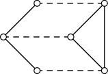
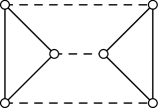
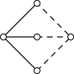
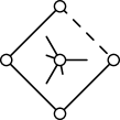
Figure 1: Pyramid, prism, theta and wheel (dashed lines represent paths)

2 A theorem on LexBFS orderings

LexBFS is a linear time algorithm of Rose, Tarjan and Lueker [26] whose input is any graph $G$ together with a vertex $s$, and whose output is a linear ordering of the vertices of $G$ starting at $s$. A linear ordering of the vertices of a graph $G$ is a LexBFS ordering if there exists a vertex $s$ of $G$ such that the ordering can be produced by LexBFS when the input is $G,s$. As the reader will soon see, we do not need to define LexBFS more precisely. The purpose of this section is to provide an alternative proof of the following result.

Theorem 2.1 (Berry and Bordat [3])

If $G$ is a non-complete graph and $z$ is the last vertex of a LexBFS ordering of $G$, then there exists a connected component $C$ of $G-N[z]$ such that for every neighbor $x$ of $z$, either $N[x]=N[z]$, or $N(x)\cap C\neq\emptyset$.

Equivalently, if we put $z$ together with its neighbors of the first type, the resultant set of vertices is a clique, a homogeneous set, and its neighborhood is a minimal separator. Such sets are called moplexes in [3] and Theorem 2.1 is stated in term of moplexes in [3]. We find it more convenient for our purpose to state it as we do. We now give an alternative proof of Theorem 2.1 for several reasons. First, it is shorter than the original proof mainly because it relies on the following nice characterization of LexBFS orderings instead of the full description of the algorithm. Second, we believe that Lemma 2.3 that we use in our proof and that was not stated explicitly before is of independent interest.

Theorem 2.2 (Brandstädt, Dragan and Nicolai [4])

An ordering $\prec$ of the vertices of a graph $G=(V,E)$ is a LexBFS ordering if and only if it satisfies the following property: for all $a,b,c\in V$ such that $c\prec b\prec a$, $ca\in E$ and $cb\notin E$, there exists a vertex $d$ in $G$ such that $d\prec c$, $db\in E$ and $da\not\in E$.

Let us strengthen a little this property for our purposes.

Lemma 2.3

Let $\prec$ be a LexBFS ordering of a graph $G=(V,E)$. Let $z$ denote the last vertex in this ordering. Then for all vertices $a,b,c\in V$ such that $c\prec b\prec a$ and $ca\in E$, there exists a path from $b$ to $c$ whose internal vertices are disjoint from $N[z]$.

Proof.

By contradiction assume there exists such a triple $c\prec b\prec a$ for which no such path exists from $b$ to $c$. Choose this triple to be minimal with respect to the sum of the positions of its elements in the ordering. Observe that since $b$ cannot be adjacent to $c$, by Theorem 2.2 there is a vertex $d$ such that $d\prec c$, $db\in E$ and $da\not\in E$. There must be a path $P$ from $c$ to $d$ whose internal vertices are disjoint from $N[z]$ otherwise $d\prec c\prec b$ would contradict the minimality of $c\prec b\prec a$. Since $db\in E$, $d$ must be a neighbor of $z$ otherwise $P\cup\{d\}$ is a path that contradicts the hypothesis. In particular, $z\neq a$. So we can apply Theorem 2.2 to the triple $d\prec a\prec z$. Thus there is a vertex $e$ such that $e\prec d$, $ea\in E$ and $ez\notin E$. But again by minimality of $c\prec b\prec a$, there exist two paths, one from $e$ to $c$ (from the triple $e\prec c\prec a$), and one from $e$ to $b$ (from the triple $e\prec b\prec a$) whose internal vertices are disjoint from $N[z]$. Since $e$ is a non-neighbor of $z$, the union of these paths contains a path from $b$ to $c$ whose internal vertices are disjoint from $N[z]$, a contradiction. ∎

With this lemma, we are now able to easily prove the aforementioned theorem.

of Theorem 2.1.

We denote by $\prec$ the LexBFS ordering. First observe that $V(G)-N[z]\neq\emptyset$, since otherwise by Theorem 2.2 $G$ is complete.

Let $x$ be a neighbor of $z$, and assume that $N(x)\subseteq N[z]$. To show that in this case $N[x]=N[z]$, let $y$ be another neighbour of $z$, and assume $xy\notin E(G)$. Either $x\prec y$ or $y\prec x$, but in both cases, Lemma 2.3 with $a=z$ implies the existence of a neighbor of $x$ that is not a neighbor of $z$, contradicting the assumption.

Now assume that $N(x)\not\subseteq N[z]$. Denote by $u$ the last vertex in $\prec$ that does not belong to $N[z]$, and by $C$ the connected component of $G-N[z]$ containing $u$. We now show that $C$ is the desired component. If $x\prec u$, then by Lemma 2.3 applied to $x\prec u\prec z$, there exists a path from $x$ to $u$ which does not meet $N[z]$, so $x$ must have a neighbor in $C$. So we may assume that $u\prec x$ and that $u$ is not adjacent to $x$. Since $x$ has a neighbor $u^{\prime}$ not belonging to $N[z]$, we must have $u^{\prime}\prec u$. Now by Lemma 2.3 applied to $u^{\prime}\prec u\prec x$, $u$ and $u^{\prime}$ belong to the same component $C$. ∎

3 Locally $\cal F$-decomposable graphs

Let $\cal F$ be a set of graphs. We are interested in graphs $G$ that admit $\cal F$-elimination orders (which is equivalent to say that every induced subgraph of $G$ has a vertex whose neighborhood is $\cal F$-free). A much stronger property is the one of being locally ${\cal F}$-free : every vertex of $G$ has a $\cal F$-free neighborhood. The following property, that sits between these two, was introduced by Maffray, Trotignon and Vušković in [23] (where it was called Property $(\star)$).

Definition 3.1

Let $\cal F$ be a set of graphs. A graph $G$ is locally $\cal F$-decomposable if for every vertex $v$ of $G$, every $F\in\cal F$ contained in $N(v)$ and every connected component $C$ of $G-N[v]$, there exists $y\in F$ such that $y$ has a non-neighbor in $F$ and no neighbors in $C$.

A class of graphs ${\cal C}$ is locally ${\cal F}$-decomposable if every graph $G\in{\cal C}$ is locally ${\cal F}$-decomposable.

It is easy to see that if a graph is locally $\cal F$-decomposable, then so are all its induced subgraphs. Therefore, for all sets of graphs $\cal F$, the class of graphs that are locally ${\cal F}$-decomposable is hereditary.

Observe that a complete graph is locally $\cal F$-decomposable for any set of graphs $\cal F$. On the other hand, a complete graph may fail to have an $\cal F$-elimination ordering, but this happens only when $\cal F$ contains graphs that are complete. This is why in the next theorem and in all the applications to come, we require that no graph of $\cal F$ is complete.

Here is now our main result. A similar theorem was given in [23] with another kind of ordering (not worth defining here) instead of LexBFS. This ordering was also lexicographic in some sense, but it could not be computed in linear time.

Theorem 3.2

If ${\cal F}$ is a set of non-complete graphs, and $G$ is a locally ${\cal F}$-decomposable graph, then every LexBFS ordering of $G$ is an $\cal F$-elimination ordering.

Proof.

Let $z$ be the last vertex of a LexBFS ordering of $G$. If $G$ is complete, then $N(z)$ is $\cal F$-free because no graph of $\cal F$ is complete. Otherwise, the connected component $C$ given by Theorem 2.1 is such that every vertex of $N(z)$ that has non-neighbors in $N(z)$ has a neighbor in $C$. So by definition of local $\cal F$-decomposability, $N(z)$ must be $\cal F$-free.

Therefore, any LexBFS ordering is an $\cal F$-elimmination ordering, because if $(v_{1},v_{2},\ldots,v_{n})$ is a LexBFS ordering, then for all $i$, $(v_{1},v_{2},\ldots,v_{i})$ is a LexBFS ordering of $G[\{v_{1},v_{2},\ldots,v_{i}\}]$ (this follows for instance from the characterization of LexBFS orderings given in Theorem 2.2). ∎

Let us now illustrate how Theorem 3.2 can be used with the simplest possible set made of non-complete graphs: ${\cal F}=\{S_{2}\}$, where $S_{2}$ is the independent graphs on two vertices. The following is of course well known, but we write its proof to illustrate our notions.

Lemma 3.3

A graph $G$ is locally $\{S_{2}\}$-decomposable if and only if $G$ is chordal.

Proof.

Suppose $G$ is not locally $S_{2}$-decomposable. Then for some $x\in V(G)$ and some connected component $C$ of $G-N[x]$, $G[N(x)]$ contains an induced subgraph $F$ isomorphic to $S_{2}$, and every vertex of $F$ has a neighbour in $C$. This clearly implies that $G$ contains a hole.

To prove the converse, suppose that $G$ contains a hole $H$, and let $y,x,z$ be three consecutive vertices of $H$. Let $C$ be the connected component of $G-N[x]$ that contains the vertices of $H-\{x,y,z\}$. Then $\{y,z\}$ is an $S_{2}$ of $N(x)$, and both $y$ and $z$ have neighbors in $C$. Therefore, $G$ is not locally $S_{2}$-decomposable. ∎

Hence, as promised in the introduction, we reobtain the proof for Theorems 1.1 and 1.2 by using Lemma 3.3 and Theorem 3.2.

4 Even-hole-free graphs and perfect graphs

In this section, we show how local decomposability can be used to provide elimination orderings and algorithms for even-hole-free graphs and some Berge graphs. A graph $G$ is Berge if $G$ and $\overline{G}$ are odd-hole-free. In the last few decades much research was devoted to the study of Berge graphs, odd-hole-free graphs and even-hole-free graphs (for surveys see [31, 33]). For all these classes global decomposition theorems are known. Most famously the celebrated proof of the Strong Perfect Graph Conjecture (which states that a graph is perfect if and only if it is Berge) obtained in 2002 by Chudnovsky, Robertson, Seymour and Thomas [7] is based on a decomposition theorem for Berge graphs. Also decomposition theorems were obtained for even-hole-free graphs [10], the most precise one by da Silva and Vušković [29]. Unfortunately, up to now, no one knows how these decomposition theorems can be used to design fast algorithms for optimization problems.

The results that we present here are in fact proved for generalizations of Berge graphs and even-hole-free graphs, the so-called signed graphs. We want to state their definitions here, because we find it interesting that they make use of the same kind of obstructions as the classes of graphs in the next section. A graph is odd-signable if there exists an assignment of $0,1$ weights to its edges that makes every chordless cycle of odd weight. A graph is even-signable if there exists an assignment of $0,1$ weights to its edges that makes every triangle of odd weight and every hole of even weight. In [32] Truemper proved a theorem that characterizes graphs whose edges can be assigned $0,1$ weights so that chordless cycles have prescribed parities. The characterization states that this can be done for a graph $G$ if and only if it can be done for all Truemper configurations and $K_{4}$’s contained in $G$. An easy consequence of this theorem when applied to odd-signable and even-signable graphs gives the following characterizations of these classes (see [11]). A sector of a wheel is a subpath of the rim of length at least 1 whose ends are adjacent to the center and whose internal vertices are not. A wheel is even if it has an even number of sectors, and it is odd if it has an odd number of sectors of length 1.

• A graph is odd-signable if and only if it is (theta, prism, even wheel)-free.

• A graph is even-signable if and only if it is (pyramid, odd wheel)-free.

We are now ready to obtain two results on vertex elimination orderings by using local $\cal F$-decomposability. These results were known already (see [28] and [23]), and were obtained by a special kind of lexicographic ordering of the vertices that is different from LexBFS (but more closely related to decomposition). Proving the existence of the ordering directly from Theorem 3.2 allows in both cases for the desired ordering to be computed in linear-time. A 4-hole is a hole of length 4.

Theorem 4.1 (da Silva and Vušković [28])

4-hole-free odd-signable graphs are locally hole-decomposable.

Theorems 4.1 and 3.2 directly imply that 4-hole-free odd-signable graphs admit a hole-elimination ordering. Theorem 4.1 is used in [28] to obtain a robust $O(n^{2}m)$-time algorithm for computing a maximum weighted clique in a 4-hole-free odd-signable graph (and hence in an even-hole-free graph). We now show how to reduce this complexity to ${O}(nm)$.

Theorem 4.2

There is an $O(nm)$-time algorithm whose input is a weighted graph $G$ and whose output is a maximum weighted clique of $G$ or a certificate proving that $G$ is not 4-hole-free odd-signable.

Proof.

Let ${\cal H}$ denotes the class of all holes and consider the following algorithm. Compute in linear time a LexBFS ordering $(v_{1},\ldots,v_{n})$ of $G$. By Theorems 3.2 and 4.1, this ordering is an ${\cal H}$-elimination ordering if $G$ is a 4-hole-free odd-signable graph. Testing whether a graph is chordal can be done in linear time [26], and hence it can be checked in ${O}(nm)$-time whether $(v_{1},\ldots,v_{n})$ is an ${\cal H}$-elimination ordering.

So, we may assume that $(v_{1},\dots,v_{n})$ is an ${\cal H}$-elimination ordering of $G$. We suppose inductively that a maximum weighted clique of $G[\{v_{1},\dots,v_{n-1}\}]$ is found in time $O((n-1)m)$. A maximum weighted clique of $G[N[v_{n}]]$ can be found in time $O(m)$ [26]. So, we now know a maximum weighted clique of $G[N[v_{n}]]$ and a maximum weighted clique of $G[\{v_{1},\dots,v_{n-1}\}]$. A maximum weighted clique among these is a maximum weighted clique of $G$. All this takes time $O((n-1)m)+O(m)=O(nm)$. ∎

We now turn our attention to Berge graphs (or more precisely to even-signable graphs that generalize them). A square-theta is a theta that contains a 4-hole. A long hole is a hole of length at least 5.

Theorem 4.3 (Maffray, Trotignon and Vušković [23])

Square-theta-free even-signable graphs are locally long-hole-decomposable.

Again, Theorems 4.3 and 3.2 directly imply that square-theta-free even-signable graphs admit a long-hole-elimination ordering. Based on Theorem 4.3 an ${O}(n^{7})$-time robust algorithm is given in [23] for computing a maximum weighted clique in a square-theta-free Berge graph (note that this class generalizes both 4-hole-free Berge graphs and claw-free Berge graphs). It relies on a long-hole-elimination ordering. With the machinery presented here, we can obtain this ordering in linear time, but unfortunately, this does not improve the overall complexity of the maximum clique algorithm.

5 Seven generalizations of chordal graphs

In this section we apply systematically our method to all possible sets made of non-complete graphs of order 3. This leads to seven classes of graphs, two of which were studied before (namely universally signable graphs and wheel-free graphs).

To describe the classes of graphs that we obtain, we need to be more specific about wheels. A wheel is a 1-wheel if for some consecutive vertices $x,y,z$ of the rim, the center is adjacent to $y$ and non-adjacent to $x$ and $z$. A wheel is a 2-wheel if for some consecutive vertices $x,y,z$ of the rim, the center is adjacent to $x$ and $y$, and non-adjacent to $z$. A wheel is a 3-wheel if for some consecutive vertices $x,y,z$ of the rim, the center is adjacent to $x$, $y$ and $z$. Observe that a wheel can be simultuneously a 1-wheel, a 2-wheel and a 3-wheel. On the other hand, every wheel is a 1-wheel, a 2-wheel or a 3-wheel. Also, any 3-wheel is either a 2-wheel or a universal wheel (that is a wheel whose center is adjacent to all vertices of the rim).

Up to isomorphism, there are four graphs on three vertices, and three of them are not complete. These three graphs (namely the independent graph on three vertices denoted by $S_{3}$, the path of length 2 denoted by $P_{3}$ and its complement denoted by $\overline{P_{3}}$) are studied in the next lemma.

Lemma 5.1

For a graph $G$ the following hold.

• $G$ is locally $\{S_{3}\}$-decomposable if and only if $G$ is (1-wheel, theta, pyramid)-free.

• $G$ is locally $\{P_{3}\}$-decomposable if and only if $G$ is 3-wheel-free.

• $G$ is locally $\{\overline{P_{3}}\}$-decomposable if and only if $G$ is (2-wheel, prism, pyramid)-free.

Proof.

To prove (i), first observe that if $G$ contains a 1-wheel, theta or pyramid $H$, then $H$ contains vertices $v,x,y,z$ such that $\{x,y,z\}$ induces an $S_{3}$, $\{x,y,z\}\subseteq N(v)$, and $H^{\prime}=H-\{v,x,y,z\}$ is a connected subgraph of $G-N[v]$ such that every vertex of $\{x,y,z\}$ has a neighbour in $H^{\prime}$.

To prove the converse, let $v\in V(G)$ be such that $G[N(v)]$ contains $S_{3}$, and $C$ a component of $G-N[v]$ such that every vertex of $S_{3}$ has a neighbor in $C$. Denote by $x,y,z$ the three members of $S_{3}$. Let $P$ be a chordless path from $x$ to $y$ with interior in $C$. Let $Q$ be a chordless path from $z$ to $z^{\prime}$, such that $V(Q)-\{z\}\subseteq C$, $z^{\prime}$ has neighbors in the interior of $P$, and is of minimum length among such paths (possibly, $Q=z=z^{\prime}$).

Suppose that at least one of $x$ or $y$ has neighbors in $Q$ (this implies that $Q$ has length at least 1). Call $w$ the vertex of $Q$ closest to $z$ along $Q$, that has neighbors in $\{x,y\}$, and suppose up to symmetry that $w$ is adjacent to $y$. Call $w^{\prime}$ the vertex of $Q$ closest to $z$ along $Q$ that has neighbors in $P-y$. Call $x^{\prime}$ the neighbor of $w^{\prime}$ in $P$, closest to $x$ along $P$. Now, $V(xPx^{\prime})\cup V(zQw^{\prime})\cup\{v,y\}$ induces a theta or a 1-wheel centered at $y$.

Therefore, we may assume that none of $x,y$ has a neighbor in $Q$. If $z^{\prime}$ has a unique neighbor in $P$, then $V(P)\cup V(Q)\cup\{v\}$ induces a theta. If $z^{\prime}$ has exactly two neighbors in $P$ that are adjacent, then $V(P)\cup V(Q)\cup\{v\}$ induces a pyramid. Otherwise, $V(P)\cup V(Q)\cup\{v\}$ contains a theta.

To prove (ii), first observe that if $G$ contains a 3-wheel $H$, then $H$ contains vertices $v,x,y,z$ such that $x,y,z$ is a $P_{3}$, $\{x,y,z\}\subseteq N(v)$, and $H^{\prime}=H-\{v,x,y,z\}$ is a connected subgraph of $G-N[v]$ such that both $x$ and $z$ have a neighbor in $H^{\prime}$. To prove the converse, let $v\in V(G)$ be such that $G[N(v)]$ contains a chordless path $xyz$, and $C$ a component of $G-N[v]$ such that $x$ and $z$ both have a neighbor in $C$. Then clearly $C\cup\{v,x,y,z\}$ contains a 3-wheel.

To prove (iii), first observe that if $G$ contains a 2-wheel, prism or pyramid $H$, then $H$ contains vertices $v,x,y,z$ such that $\{x,y,z\}$ induces a $\overline{P_{3}}$, $\{x,y,z\}\subseteq N(v)$, and $H^{\prime}=H-\{v,x,y,z\}$ is a connected subgraph of $G-N[v]$ such that every vertex of $\{x,y,z\}$ has a neighbor in $H^{\prime}$.

To prove the converse, let $v\in V(G)$ be such that $G[N(v)]$ contains $\overline{P_{3}}$, and $C$ a component of $G-N[v]$ such that every vertex of $\overline{P_{3}}$ has a neighbor in $C$. Denote by $x,y,z$ the vertices of $\overline{P_{3}}$ in such a way that $xy$ is the only edge of $G[\{x,y,z\}]$. Let $P$ be a path from $x$ to $y$ with interior in $C$ whose unique chord is $xy$. Let $Q$ be a chordless path from $z$ to $z^{\prime}$, such that $V(Q)-\{z\}\subseteq C$, $z^{\prime}$ has neighbors in the interior $P$, and is of minimum length among such paths (possibly, $Q=z=z^{\prime}$).

Suppose that at least one of $x$ or $y$ has neighbors in $Q$. Call $w$ the vertex of $Q$ closest to $z$ along $Q$, that has neighbors in $\{x,y\}$, and suppose up to symmetry that $w$ is adjacent to $y$. Call $w^{\prime}$ the vertex of $Q$ closest to $z$ along $Q$ that has neighbors in $P-y$. Call $x^{\prime}$ the neighbor of $w^{\prime}$ in $P$, closest to $x$ along $P$. Now, $V(xPx^{\prime})\cup V(zQw^{\prime})\cup\{v,y\}$ induces a 2-wheel centered at $y$.

Therefore, we may assume that none of $x,y$ has a neighbor in $Q$. If $z^{\prime}$ has a unique neighbor in $P$, then $V(P)\cup V(Q)\cup\{v\}$ induces a pyramid or a 2-wheel (when $P$ has length 2). If $z^{\prime}$ has exactly two neighbors in $P$ that are adjacent, then $V(P)\cup V(Q)\cup\{v\}$ induces a prism. Otherwise, $V(P)\cup V(Q)\cup\{v\}$ contains a pyramid. ∎

The next lemma allows us to combine the results of the previous one.

Lemma 5.2

Let ${\cal F},{\cal F}^{\prime},{\cal H},{\cal H^{\prime}}$ be sets of graphs such that $\cal F$ and $\cal F^{\prime}$ contain only non-complete graphs. Suppose that the class of locally ${\cal F}$-decomposable graphs is equal to the class of ${\cal H}$-free graphs, and that the class of locally ${\cal F}^{\prime}$-decomposable graphs is equal to the class of ${\cal H}^{\prime}$-free graphs. Then, the class of locally $({\cal F}\cup{\cal F}^{\prime})$-decomposable graph is is equal to the class of $({\cal H}\cup{\cal H}^{\prime})$-free graphs.

Proof.

Suppose that $G$ is locally $({\cal F}\cup{\cal F}^{\prime})$-decomposable. From the definition of local decomposability, it follows that $G$ is locally ${\cal F}$-decomposable and locally ${\cal F}^{\prime}$-decomposable. Hence, $G$ is both ${\cal H}$-free and ${\cal H}^{\prime}$-free. It is therefore $({\cal H}\cup{\cal H}^{\prime})$-free.

Suppose conversely that $G$ is $({\cal H}\cup{\cal H}^{\prime})$-free. Then $G$ is ${\cal H}$-free and ${\cal H}^{\prime}$-free. It is thereofore locally ${\cal F}$-decomposable and locally ${\cal F}^{\prime}$-decomposable. From the definition of local decomposability, it follows that $G$ is locally $({\cal F}\cup{\cal F}^{\prime})$-decomposable. ∎

$i$	Class ${\cal C}_{i}$	${\cal F}_{i}$	Neighborhood
1	(1-wheel, theta, pyramid)-free	$\left\{\parbox[c]{15.6491pt}{\includegraphics[width=14.22636pt]{fig-7.pdf}}\right\}$	no stable set of size 3
2	3-wheel-free	$\left\{\parbox[c]{15.6491pt}{\includegraphics[width=14.22636pt]{fig-8.pdf}}\right\}$	disjoint union of cliques
3	(2-wheel, prism, pyramid)-free	$\left\{\parbox[c]{15.6491pt}{\includegraphics[width=14.22636pt]{fig-9.pdf}}\right\}$	complete multipartite
4	(1-wheel, 3-wheel, theta, pyramid)-free	$\left\{\parbox[c]{36.98866pt}{\includegraphics[width=14.22636pt]{fig-7.pdf}\,, \includegraphics[width=14.22636pt]{fig-8.pdf}}\right\}$	disjoint union of at most two cliques
5	(1-wheel, 2-wheel, prism, theta, pyramid)-free	$\left\{\parbox[c]{36.98866pt}{\includegraphics[width=14.22636pt]{fig-7.pdf}\,, \includegraphics[width=14.22636pt]{fig-9.pdf}}\right\}$	stable sets of size at most 2 with all possible edges between them
6	(2-wheel, 3-wheel, prism, pyramid)-free	$\left\{\parbox[c]{36.98866pt}{\includegraphics[width=14.22636pt]{fig-8.pdf}\,, \includegraphics[width=14.22636pt]{fig-9.pdf}}\right\}$	clique or stable set
7	(wheel, prism, theta, pyramid)-free	$\left\{\parbox[c]{62.59596pt}{\includegraphics[width=14.22636pt]{fig-7.pdf}\,, \includegraphics[width=14.22636pt]{fig-8.pdf}\,, \includegraphics[width=14.22636pt]{fig-9.pdf}}\right\}$	clique or stable set of size 2
8	hole-free	$\left\{\parbox[c]{8.5359pt}{\ \includegraphics[height=14.22636pt]{fig-16.pdf}\ }\right\}$	clique

Table 1: Eight classes of graphs

Figure 2: Inclusion for several classes of graphs. An arrow from $A$ to $B$ means “$A$ is contained in $B$”. Arrows arising from transitivity are not represented.

Table 1 describes eight different classes of graphs ${\cal C}_{1},\dots,{\cal C}_{8}$, all defined by excluding induced subgraphs described in the second column of the table (one of them is the class of chordal graphs that we put back to have a complete picture). The third column describes a class ${\cal F}_{i}$. The last column describes the class of ${\cal F}_{i}$-free graphs. Inclusions between our classes and several known classes are represented in Figure 2 (where the diamond is the graph obtained from $K_{4}$ by removing one edge, a cap is cycle of length at least 5 with a unique chord joining two vertices at distance 2 on the cycle, a d-hole is 3-wheel such that the center has degree 3, and the claw is $K_{1,3}$). Observe that a d-hole is also a 2-wheel. The following theorem follows directly from Lemmas 5.1, 5.2 and 3.3.

Theorem 5.3

For $i=1,\dots,8$, let ${\cal C}_{i}$ and ${\cal F}_{i}$ be the classes defined as in Table 1. For $i=1,\dots,8$, the class ${\cal C}_{i}$ is exactly the class of locally ${\cal F}_{i}$-decomposable graphs.

With Theorem 3.2, this directly implies the following.

Theorem 5.4

For $i=1,\dots,8$, let ${\cal C}_{i}$ and ${\cal F}_{i}$ be the classes defined as in Table 1. Then every LexBFS ordering of a graph of ${\cal C}_{i}$ is an ${\cal F}_{i}$-elimination ordering.

Known classes

We now describe the two classes of graphs from Table 1 that (apart from chordal graphs) were studied before. The first one is ${\cal C}_{7}$, i.e. graphs that contain no Truemper configuration, or equivalently by Theorem 5.4, graphs that are ${\cal F}_{7}$-locally decomposable. These are studied in [9], where they are called universally signable graphs. The existence of a vertex whose neighborhood is ${\cal F}_{7}$-free given by Theorem 5.4 is exactly the following theorem from [9], that was originally proved through a global decomposition theorem. Theorem 5.4 provides a shorter proof as well as an algorithm that outputs the order that does not rely on global decomposition. In the next subsection, we study several algorithmic consequences.

Theorem 5.5 (Conforti, Cornuéjols, Kapoor and Vušković [9])

Every non-empty universally signable graph contains a simplicial vertex or a vertex of degree $2$.

The second class that was studied previously is the class of wheel-free graphs and its super-class ${\cal C}_{2}$. These might have interesting structural properties, as suggested by several subclasses, see [1] for example for a list of them. The next theorem (which follows from Theorem 5.4 for $i=2$) states the only non-trivial property that is known to be satisfied by all wheel-free graphs. The original proof (due to Chudnovsky who communicated it to us but did not publish it) is by induction, and the proof relying on our method is much shorter.

Theorem 5.6 (Chudnovsky [5])

Every non-empty 3-wheel-free graph contains a vertex whose neighborhood is a disjoint union of cliques.

The following corollary extends a well-known fact: a chordal graph $G$ has at most $n$ maximal cliques.

Corollary 5.7

A 3-wheel-free graph $G$ has at most $m$ maximal cliques.

Proof.

Induction on $m$. By Theorem 5.6, consider a vertex $v$ of degree $d$ whose neighborhood is a disjoint union of cliques. By the induction hypothesis, $G-v$ has at most $m-d$ maximal cliques, and because of its neighborhhood, $v$ is in at most $d$ maximal cliques. ∎

Consequences

$i$	$\chi$-bounded	Max clique	Coloring
1	$f(x)=O(x^{2}/\log x)$	NP-hard [25]	NP-hard [18]
2	No [35]	$O(nm)$ [26]	NP-hard [22]
3	No [35]	$O(nm)$	NP-hard [22]
4	$f(x)=2x-1$	$O(n+m)$	?
5	$f(x)=2x-1$	$O(nm)$	?
6	No [35]	$O(n+m)$	NP-hard [22]
7	$f(x)=\max(3,x)$ [9]	$O(n+m)$	$O(n+m)$
8	$f(x)=x$ [12]	$O(n+m)$ [26]	$O(n+m)$ [26]

Table 2: Several properties of classes defined in Table 1

Table 2 describes several properties of the classes defined in Table 1. We indicate a reference for the properties that are already known, or follow easily from the given references. Let us now explain and prove all these properties.

Let us analyze the column “$\chi$-bounded” of Table 2. A hereditary class of graphs is $\chi$-bounded (see [17]) if for some function $f$, every graph $G$ in the class satisfies $\chi(G)\leq f(\omega(G))$. The column indicates whether the class $C_{i}$ is $\chi$-bounded, and if so, gives the smallest known function proving so. Classes ${\cal C}_{2},{\cal C}_{3}$ and ${\cal C}_{6}$ are not $\chi$-bounded because they contain all triangle-free graphs, and these may have arbitrarily large chromatic number as first shown by Zykov [35]. For classes ${\cal C}_{1},{\cal C}_{4}$ and ${\cal C}_{5}$, we may rely on degeneracy. Say that a hereditary class of graphs is $\omega$-degenerate if there exists a function $g$ such that every non-empty graph in the class has a vertex of degree at most $g(\omega(G))$. It is easy to check that by the greedy coloring algorithm, if a hereditary class of graphs is $\omega$-degenerate with a non-decreasing function $g$, then it is $\chi$-bounded with function $g+1$. The function given for classes ${\cal C}_{4}$ and ${\cal C}_{5}$ follows from the fact that these classes are clearly $\omega$-degenerate with function $g(x)=2x-2$. For the class ${\cal C}_{1}$, we use Ramsey theory. Kim [19] proved that for some constant $c$, every graph on $ct^{2}/\log t$ vertices admits a stable set of size 3 or a clique of size $t$. Therefore, the vertex whose neighborhood is $S_{3}$-free in any graph in ${\cal C}_{1}$ proves that ${\cal C}_{1}$ is $\omega$-degenerate with function $g(x)=O(x^{2}/\log x)$. Observe that the results in this paragraph just improve bounds. Indeed, a theorem due to Kühn and Osthus [21] proves that theta-free graphs (and therefore graphs in ${\cal C}_{1}$, ${\cal C}_{4}$ and ${\cal C}_{5}$) are $\omega$-degenerate, but their function is quite big.

Let us now analyze the column “Max clique” of Table 2, that gives the best complexity of finding a maximum weighted clique in a graph of the corresponding class. By a result of Poljak [25], it is NP-hard to compute a maximum stable set in a triangle-free graph. Rephrased in the complement, it is NP-hard to compute a maximum clique in an $S_{3}$-free graph, and therefore in graphs from ${\cal C}_{1}$. Finding a maximum weighted clique in ${\cal C}_{2}$ is easy as follows: for every vertex $v$, look for a maximum weighted clique in $N(v)$, and choose the best clique among these. This can be implemented by running $n$ times the $O(n+m)$ algorithm of Rose, Tarjan and Lueker, because $N(v)$ is chordal for every $v$. In fact, this algorithm works in the larger class of universal-wheel-free graphs.

For ${\cal C}_{4}$, we need to be careful about the complexity analysis. Here is an algorithm that finds a maximum (weighted) clique in $G\in{\cal C}_{4}$. First by Theorem 5.4, we find in linear time an $\{S_{3},P_{3}\}$-elimination ordering of $G$, say $(v_{1},\dots,v_{n})$. This means that in $G[\{v_{1},\dots,v_{i}\}]$, $N(v_{i})$ is a disjoint union of at most two cliques. We now show that, having this order, we can compute a maximum clique in time $O(m)$. We may assume that $G$ is connected (otherwise we work on components separately), so $m\geq n-1$. Suppose inductively that a maximum clique of $G[\{v_{1},\dots,v_{n-1}\}]$ is found in time $O(m-d(v_{n}))$. We now take the vertices of $N(v_{n})$ one by one. We give name $x$ and label $X$ to first one, and check whether the next ones are adjacent to $x$. If so, we give them label $X$. If some are not adjacent to $x$, we give name $y$ and label $Y$ to the first one that we meet. The next vertices receive label $X$ or $Y$ according to their adjacency to $x$ or $y$. Note that exactly one of these adjacencies must occur, since $N(v_{n})$ is the union of at most two cliques. At the end of this loops, the vertices with label $X$ and $Y$ form at most two cliques in $N(v_{n})$. They are identified in time $O(d(v_{n}))$. So, we now know all the maximal cliques of $G[N[v_{n}]]$ and a maximum clique of $G[\{v_{1},\dots,v_{n-1}\}]$. A maximum clique among these is a maximum clique of $G$. All this takes time $O(m-d(v_{n}))+O(d(v_{n}))=O(m)$. Observe that this algorithm relies on a constant time checking of the adjacency, so it needs the graph to be represented by an adjacency matrix. Therefore, the time complexity is $O(n+m)$, but the space complexity is $O(n^{2})$. Observe also that this algorithm is not robust. If the input graph is not in ${\cal C}_{4}$, the output is a set of vertices, and if it is a clique, we cannot be sure that it has maximum weight. Since ${\cal C}_{7}$ is a subclass of ${\cal C}_{4}$, we obtain an algorithm for the maximum clique problem for universally signable graphs that is fastest than the $O(nm)$-time algorithm that follows from [9].

For class ${\cal C}_{6}$, the algorithm is similar to the previous one. We have to find a maximum clique in $N(v_{n})$ in time $O(d(v_{n}))$. It is easy to verify quickly whether the neighbohood of $v_{n}$ is a clique or a stable set, and in both cases, it is immediate to find in time $O(d(v_{n}))$ a maximum weighted clique in it. We omit further details.

For ${\cal C}_{3}$ (that contains ${\cal C}_{5}$), the algorithm is similar to the previous one, except that we rely on a $\{\overline{P_{3}}\}$-elimination ordering of $G$ instead of an $\{S_{3},P_{3}\}$-elimination ordering. As a result, the neighborhood of the last vertex $v$ is complete multipartite. We do not know how to find a maximum clique in $N(v)$ in time $O(d(v))$, so we do not know how to obtain a linear time algorithm. Instead, we look for a maximum clique in $N(v)$ in time $O(m)$, and therefore the overall complexity is $O(nm)$.

Let us now analyze the column “Coloring” of Table 2, that gives the best complexity for coloring a graph of the corresponding class. Since the edge-coloring problem is NP-hard [18], it follows that coloring line graphs is NP-hard, and therefore, so is coloring claw-free graphs (that are all in ${\cal C}_{1}$). Classes ${\cal C}_{2},{\cal C}_{3}$ and ${\cal C}_{6}$ contain all triangle-free graphs, that are NP-hard to color as proved by Preissmann and Maffray [22]. For ${\cal C}_{7}$, we first try to find a 2-coloring of the graph by the classical BFS algorithm. If it does not exist, we look for a $\max(3,\omega(G))$-coloring of the input graph $G$ as follows. By Theorem 5.4 we obtain an $\{S_{3},P_{3},\overline{P_{3}}\}$-elimination ordering in linear time. As a result, the neighborhood of the last vertex of the ordering is a clique or has size 2. We remove the last vertex $v$, color recursively the remaining vertices, and give some available color to $v$.

6 Open questions

Addario-Berry, Chudnovsky, Havet, Reed and Seymour [2] proved that every even-hole-free graph admits a vertex whose neighborhood is the union of two cliques. We wonder whether this result can be proved by some search algorithm.

Corollary 5.7 suggests that a linear time algorithm for the maximum clique problem might exists in ${\cal C}_{2}$, but we could not find it.

We are not aware of a polynomial time coloring algorithm for graphs in ${\cal C}_{4}$ or ${\cal C}_{5}$, but it would be surprising to us that it exists.

Since class ${\cal C}_{1}$ generalizes claw-free graphs, it is natural to ask which of the properties of claw-free graphs it has, such as a structural description (see [8]), a polynomial time algorithm for the maximum stable set (see [13]), approximation algorithms for the chromatic number (see [20]), a polynomial time algorithm for the induced linkage problem (see [14]), and a polynomial $\chi$-binding function (see [17]). Also we wonder whether theta-free graphs are $\chi$-bounded by a polynomial (quadratic?) function (recall that in [21], they are proved to be $\chi$-bounded).

In [9], an $O(nm)$ time algorithm is described for the maximum weighted stable set problem in ${\cal C}_{7}$. Since the class is a simple generalization of chordal graphs, we wonder whether a linear time algorithm exists.

Ackowledgement

Thanks to Maria Chudnovsky for indicating to us Theorem 5.6 and its proof, which was the starting point of this research. Thanks to Michael Rao and two anonymous referees for comments that helped improve this paper.

References

- [1] P. Aboulker, M. Radovanović, N. Trotignon, and K. Vušković. Graphs that do not contain a cycle with a node that has at least two neighbors on it. SIAM Journal on Discrete Mathematics, 26(4):1510–1531, 2012.
- [2] L. Addario-Berry, M. Chudnovsky, F. Havet, B. Reed, and P. Seymour. Bisimplicial vertices in even-hole-free graphs. Journal of Combinatorial Theory, Series B, 98(6):1119–1164, 2008.
- [3] A. Berry and J.-P. Bordat. Separability generalizes Dirac’s theorem. Discrete Applied Mathematics, 84:43–53, 1998.
- [4] A. Brandstädt, F.F. Dragan, and F. Nicolai. LexBFS-orderings and powers of chordal graphs. Discrete Mathematics, 171(1–3):27–42, 1997.
- [5] M. Chudnovsky. Personal communication. 2012.
- [6] M. Chudnovsky, G. Cornuéjols, X. Liu, P. Seymour, and K. Vušković. Recognizing Berge graphs. Combinatorica, 25(2):143–186, 2005.
- [7] M. Chudnovsky, N. Robertson, P. Seymour, and R. Thomas. The strong perfect graph theorem. Annals of Mathematics, 164(1):51–229, 2006.
- [8] M. Chudnovsky and P. Seymour. Clawfree graphs. IV. Decomposition theorem. Journal of Combinatorial Theory, Series B, 98(5):839–938, 2008.
- [9] M. Conforti, G. Cornuéjols, A. Kapoor, and K. Vušković. Universally signable graphs. Combinatorica, 17(1):67-77, 1997.
- [10] M. Conforti, G. Cornuéjols, A. Kapoor, and K. Vušković. Even-hole-free graphs Part I: Decomposition theorem. Journal of Graph Theory, 39:6–49, 2002.
- [11] M. Conforti, G. Cornuéjols, A. Kapoor, and K. Vušković. Even and odd holes in cap-free graphs. Journal of Graph Theory, 30:289-308, 1999.
- [12] G.A. Dirac. On rigid circuit graphs. Abhandlungen aus dem Mathematischen Seminar der Universität Hamburg, 25:71–76, 1961.
- [13] Y. Faenza, G. Oriolo, and G. Stauffer. An algorithmic decomposition of claw-free graphs leading to an )-algorithm for the weighted stable set problem. Proceedings of the Twenty-Second Annual ACM-SIAM Symposium on Discrete Algorithms, SODA 2011, San Francisco, California, USA, January 23–25, 2011. SIAM, 2011, Dana Randall editor, pages 630–646.
- [14] J. Fiala, M. Kaminski, B. Lidický, and D. Paulusma. The -in-a-path problem for claw-free graphs. Algorithmica, 62(1–2):499–519, 2012.
- [15] D.R. Fulkerson, and O.A. Gross. Incidence matrices and interval graphs. Pacific J. Math., 15:835–855, 1965.
- [16] M. Grötschel, L. Lovász, and A. Schrijver. Geometric Algorithms and Combinatorial Optimization. Springer Verlag, 1988.
- [17] A. Gyárfás. Problems from the world surrounding perfect graphs. Zastowania Matematyki Applicationes Mathematicae, 19:413–441, 1987.
- [18] I. Holyer. The NP-completeness of some edge-partition problems. SIAM Journal on Computing, 10(4):713–717, 1981.
- [19] J.H. Kim. The Ramsey number has order of magnitude . Random Structures and Algorithms, 7(3):173–208, 1995.
- [20] A. King. Claw-free graphs and two conjectures on , , and . PhD thesis, McGill University, 2009.
- [21] D. Kühn and D. Osthus. Induced subdivisions in -free graphs of large average degree. Combinatorica, 24(2):287–304, 2004.
- [22] F. Maffray and M. Preissmann. On the NP-completeness of the -colorability problem for triangle-free graphs. Discrete Mathematics, 162:313–317, 1996.
- [23] F. Maffray, N. Trotignon, and K. Vušković. Algorithms for square--free Berge graphs. SIAM Journal on Discrete Mathematics, 22(1):51–71, 2008.
- [24] I. Parfenoff, F. Roussel, and I. Rusu. Triangulated neighbourhoods in -free Berge graphs. Proceedings of International Workshop on Graph-Theoretic Concepts in Computer Science, 402–412, 1999.
- [25] S. Poljak. A note on the stable sets and coloring of graphs. Commentationes Mathematicae Universitatis Carolinae, 15:307–309, 1974.
- [26] D.J. Rose, R.E. Tarjan, and G.S. Lueker. Algorithmic aspects of vertex elimination on graphs. SIAM Journal on Computing, 5:266–283, 1976.
- [27] F. Roussel, and I. Rusu. A linear algorithm to color i-triangulated graphs. Information Processing Letters, 70(2):57–62, 1999.
- [28] M.V.G. da Silva and K. Vušković. Triangulated neighborhoods in even-hole-free graphs. Discrete Mathematics, 307(9-10):1065–1073, 2007.
- [29] M.V.G. da Silva and K. Vušković. Decomposition of even-hole-free graphs with star cutsets and 2-joins. Journal of Combinatorial Theory B, 103:144–183, 2013.
- [30] R.E. Tarjan. Decomposition by clique separators. Discrete Mathematics, 55:221-232, 1985.
- [31] N. Trotignon. Perfect graphs: a survey. arXiv:1301.5149, 2013.
- [32] K. Truemper. Alpha-balanced graphs and matrices and GF(3)-representability of matroids. Journal of Combinatorial Theory B, 32:112-139, 1982.
- [33] K. Vušković, Even-hole-free graphs: a survey. Applicable Analysis and Discrete Mathematics, 4:219–240, 2010.
- [34] K. Vušković. The world of hereditary graph classes viewed through Truemper configurations. Surveys in Combinatorics, London Mathematical Society Lecture Note Series, Cambridge University Press, 265-326, 2013.
- [35] A.A. Zykov. On some properties of linear complexes. Matematicheskii Sbornik, 24(2):163–188, 1949. In Russian.