INTEGRAL FIELD SPECTROSCOPY OF THE BRIGHTEST KNOTS OF HH 223 IN L723

Abstract

HH 223 is the optical counterpart of a larger scale H₂ outflow, driven by the protostellar source VLA 2A, in L723. Its poorly collimated and rather chaotic morphology suggested the Integral Field Spectroscopy (IFS) as an appropriate option to map the emission for deriving the physical conditions and the kinematics. Here we present new results based on the IFS observations made with the INTEGRAL system at the WHT. The brightest knots of HH 223 ($\sim$ 16 arcsec, $\simeq$ 0.02 pc at a distance of 300 pc) were mapped with a single pointing in the spectral range 6200–7700 Å. We obtained the emission-line intensity maps for H$\alpha$, [N ii] 6584 Å and [S ii] 6716, 6731 Å, and explored the distribution of the excitation and electron density from [N ii]/H$\alpha$, [S ii]/H$\alpha$, and [S ii] 6716/6731 line-ratio maps. Maps of the radial velocity field were obtained. We analysed the 3D-kinematics by combining the knot radial velocities, derived from IFS data, with the knot proper motions derived from multi-epoch, narrow-band images. The intensity maps built from IFS data reproduced well the morphology found in the narrow-band images. We checked the results obtained from previous long-slit observations with those derived from IFS spectra extracted with a similar spatial sampling. At the positions intersected by the slit, the physical conditions and kinematics derived from IFS are compatible with those derived from long-slit data. In contrast, significant discrepancies were found when the results from long-slit data were compared with the ones derived from IFS spectra extracted at positions shifted a few arcsec from those intersected by the slit. This clearly revealed IFS observations as the best choice to get a reliable picture of the HH emission properties.

1 INTRODUCTION

The Herbig-Haro object 223 of the Reipurth Catalogue (Reipurth, 1994) is a knotty, undulating emission of $\sim$ 30 arcsec length, and corresponds to the brightest optical counterpart of a large-scale ($\sim$ 5.5 arcmin) H₂ outflow. The outflow is located in the dark cloud Lynds 723 (L723), at a distance of 300 $\pm$ 150 pc (Goldsmith et al., 1984). It is associated with the low-mass multiple system VLA 2 (, 1991), being one of the components of this system (VLA 2A) the outflow exciting source (Carrasco-González et al., 2008). For a more detailed description of the region and the nomenclature of the outflow knots, see López et al. (2010a) and references therein.

In a previous work (López et al., 2009), we performed long-slit spectroscopy in the spectral range 5800-8300 Å along two slit positions, which intersect the peaks of the bright HH 223 knots (A to E), including emission from the low-brightness nebula surrounding the knots. The spectra of the knots are characteristic of shock-excited gas with an intermediate/high degree of excitation. The radial velocities derived for the knots are highly blueshifted relative to the ambient gas cloud, and supersonic, as expected for a HH optical jet. Significant changes in the physical conditions (namely, in the excitation, ionization and electron density) were found as we move a few arcsec along the slits. In addition, two velocity components seem to be present at several of the positions intersected by the slits. It is likely that, at these positions, there is contribution to the emission from both the shocked jet gas and the ambient gas, dragged and accelerated by the supersonic outflow. Note, however, that we sampled partially the spatial emission of the HH 223 knots and interknot nebula by means of the long-slit observations. In contrast, Integral Field Spectroscopy (IFS) appears to be the appropriate tool to get a wider spatial coverage that includes the whole spatial knot/interknot emission. This technique has proven to be very efficient to study the kinematics and physical conditions, mainly in the case of Herbig-Haro objects having a poorly collimated morphology (see, e. g. HH 262, López et al., 2008; HH 110, López et al., 2010b).

Taking advantage of the capabilities of INTEGRAL (Arribas et al., 1998), we made a single-pointing observation in HH 223, covering the emission of its brightest knots (A to D). From these data, we obtained the morphology in several emission lines, the kinematics and the physical conditions of HH 223. In addition, we were able to compare the results derived from IFS data with those obtained from narrow-band and long-slit observations using similar spatial and spectral resolutions. This experiment gave us the opportunity to test whether a partial sampling of the emission performed from long-slit data might mask some behaviours of the actual spatial distribution of the physical conditions in HHs such as HH 223, with a poor collimated and rather chaotic morphology.

We also present in this paper the 3D kinematics of the brightest HH 223 knots derived by combining the INTEGRAL data (radial velocity) with narrow-band H$\alpha$ images obtained at three different epochs (proper motions).

2 OBSERVATIONS AND DATA REDUCTION

2.1 INTEGRAL FIELD SPECTROSCOPY

The 4.2 m William Herschel Telescope (WHT) of the Observatorio del Roque de los Muchachos (ORM, La Palma, Spain) was used in combination with the INTEGRAL fiber optics system (Arribas et al., 1998) and the WYFFOS spectrograph (Bingham et al., 1996). INTEGRAL links the Nasmyth focus of the WHT with the slit of WYFFOS through three optical fiber bundles. At the focal plane, the fibers of these three bundles are arranged into two groups, one forming a central rectangle, and the other an outer ring mapping the sky. The three bundles can be interchanged online depending on the scientific program or the prevailing seeing conditions, as they have different spatial sampling and coverage. More information about INTEGRAL bundles and performances can be found at the INTEGRAL web page. The data discussed in this paper were obtained with the standard bundle 2 (STD2). STD2 consists of 219 fibers (189 science and 30 sky fibers), each of 0.9 arcsec in diameter on the sky and covering a field of view (FOV) of 16 $\times$ 12  arcsec².

The observations were made on 2009 May 25 as a backup program of the science verification allocated time for a new equalized fiber bundle for INTEGRAL. The WYFFOS spectrograph was equipped with a 1200 groove mm^-1 grating (centered on $\lambda\ 7000$ Å) and a EEV mosaic (two EEV-42-80 thinned and AR coated CCDs) of 4308$\times$ 4200 pixels of 13.5 $\mu$m in size, giving a linear dispersion of about 0.4 Å pixel^-1 in the spectral range $\sim$ 6180–7700 Å. With this configuration, and pointing to the brightest knots of HH 223 ($\alpha$=19^h 17^m 57$\aas@@fstack{s}7$, $\delta$=+19$\degr$ 11$\arcmin$ 52$\arcsec$), five exposures of 1800 s each and one exposure of 900 s were taken to get a total effective integration time of 2.75 hr. This single pointing covers the brightest HH 223 knots (HH 223-A to -D) and the low-brightness nebular emission surrounding these knots, as illustrated in Fig. 1, where the spectrum extracted from each fiber, in a wavelength range around H$\alpha$, is overplotted on the HH 223 H$\alpha$ narrow-band image. The knots are labeled as in López et al. (2006).

Figure 1: (a) H$\alpha$ narrow-band image of the HH 223 field obtained at the Nordic Optical Telescope (NOT) on 2009 May 18. The white rectangle includes the region mapped with the IFS single pointing. (b) Two-dimensional distribution diagram of the observed spectra in the spectral window 6540-6590 Å, which includes the H$\alpha$ and [N ii] 6548, 6584 Å emission lines. The spectra have been rescaled to show better the line profile, and are overplotted onto the H$\alpha$ narrow-band. Labels of knots identification (following López et al., 2006) are included. The offsets are relative to the centre of the field covered by IFS.

The data were reduced using IRAF standard routines (see e. g. García-Lorenzo et al., 2005 for a description of the reduction of IFS data from fiber-based instruments). We obtained typical wavelength calibration errors of 0.1 Å, which give velocity uncertainties of about $\pm$ 4.5 km s^-1 for H$\alpha$. The differential atmospheric refraction was estimated according to the model given by (1973), being this effect negligible for the HH 223 observations. The night was photometric according to the Mercator Telescope measurements and the seeing was around 1 arcsec.

2.2 Narrow-band CCD images

Deep narrow-band CCD images of L723, covering a field of $\sim~{}5~{}\times$ 5 arcmin² that includes HH 223 were obtained at three different epochs (2004 July 20, 2007 July 14, and 2009 May 18), suitable to measure proper motion displacements of the knots. The Andalucia Faint Object Spectrograph and Camera (ALFOSC) was used on the 2.6 m Nordic Optical Telescope (NOT) at the ORM. The image scale was 0.188 arcsec pixel^-1. The filter used had a central wavelength of 6564 Å and a bandpass of 33 Å, which mainly included emission from the H$\alpha$ line, with some contamination from the [N ii] $\lambda$ 6548 Å emission line. All the images were processed as described in López et al. (2006) for the 2004 observing run. The IAA Guaranteed Observing Time with ALFOSC was used for the observing run of 2009.

3 IFS RESULTS

3.1 IFS imaging: spatial distribution of physical conditions

Emissions from H$\alpha$, [N ii] and [S ii] $\lambda$ 6716, 6731 Å were detected in all the fibers covering the HH 223 knots and its surrounding nebula mapped with INTEGRAL. Other characteristic HH emission lines included in the observed wavelength range ([O i] doublet, [Fe ii] $\lambda$ 7155 Å and [O ii] $\lambda$ 7300 Å doublet) were only detected in a few fibers, located around the peak positions of the brightest knots A and B.

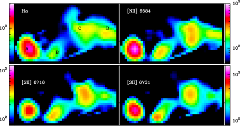
Figure 2: IFS-derived narrow-band images for several emission lines (H$\alpha$, [N ii]$\lambda$ 6584 Å and [S ii]$\lambda$ 6716, 6731 Å). For each position, the flux of the line was obtained from a Gaussian fit to the line profile, after subtracting a continuum, obtained from the adjacent wavelength range free of line emission. The flux scale is in counts.

Figure 2 shows the morphology of HH 223 for the H$\alpha$, [N ii] $\lambda$ 6584 Å and [S ii] $\lambda$ 6716, 6731 Å emission lines obtained from IFS data. To generate these narrow-band images, a two-dimensional interpolation was applied using the IDA package (García-Lorenzo et al., 2002). In particular, an ASCII file with the actual position of the fiber and the corresponding spectral feature was transformed to obtain a regularly spaced rectangular grid. In this way, we built up narrow-band images with a field of view of 47$\times$27 pixels ($\sim$ 14 arcsec $\times$ 8 arcsec) with a spatial scale of 0.3 arcsec pixel^-1 that can be treated with standard astronomical software packages.

The IFS maps (Fig. 2) are in good agreement with previous CCD narrow-band H$\alpha$ and [S ii] images of HH 223 (López et al., 2006). In the four emission lines considered, the IFS maps reproduce the undulating, knotty structure of the emission, surrounded by a low-brightness nebula that had already been found in the narrow-band, CCD images. Note however that the IFS data allowed us to map separately the emission coming from the H$\alpha$ and [N ii] lines, as well as the two lines of the [S ii] doublet. We can now observe the close similarity between the brightness distribution of the [S ii] and [N ii] maps. In contrast, the comparison of H$\alpha$ and [N ii] IFS maps shows differences in the morphology and relative brightness of the knots. In particular, knot C shows a somewhat different morphology in [N ii] (with two, north-south, condensations of similar brightness) and H$\alpha$ (where the southern condensation is fainter than the northern one). Furthermore, knots B and C show a higher [N ii]/H$\alpha$ brightness ratio than knot A. As we will discuss later, these signatures are the result of differences in gas excitation through the HH 223 emission, which were only outlined from long-slit spectroscopy.

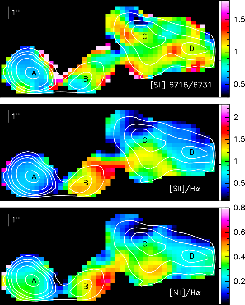
Figure 3: [S ii]6716/6731 (top), [S ii] (6716+6731)/H$\alpha$ (middle) and [N ii] 6584/H$\alpha$ (bottom) line-ratio maps obtained from the IFS-narrow-band images, blanking the regions with a SNR $\leq$ 3. Contours from the H$\alpha$ IFS image are overlapped to help with the identification of the knot condensations.

Line-ratio maps of the emission lines widely used for nebular diagnosis ([S ii] (6716+6731)/H$\alpha$ and [N ii] 6584/H$\alpha$ for excitation, and [S ii] 6716/6731 for electron density) were obtained from the IFS-narrow-band images, and are displayed in Fig. 3.

For all the mapped region, which included emission from knots and from the low-brightness interknot nebula, the values of the [S ii]/H$\alpha$ line ratio range from 0.6 to 1.4, and those of the [N ii]/H$\alpha$, from 0.2 to 0.5. According to the [S ii]/H$\alpha$ vs. [N ii]/H$\alpha$ diagnostic diagrams (see e. g. Cantó, 1981), these values are found in HH objects, where the emission is produced by shocks. In fact, the values derived for the [S ii]/H$\alpha$ line-ratio correspond to the spectra with an intermediate/high degree of excitation, following the classification for HHs proposed by Raga et al. (1996), which distinguished the low (with a [S ii]/H$\alpha$ $\geq$ 1.5) from the intermediate/high excitation spectra. The spatial distribution of the electron density ($n_{\mathrm{e}}$) is outlined in the [S ii] 6716/6731 line ratio map. Values of the sulphur line ratio range from 0.6 to 1.2, which correspond to $n_{\mathrm{e}}$ ranging from 0.24 to 4.2$\times$10³ cm^-3 ($n_{\mathrm{e}}$ derived using the TEMDEN task of the IRAF/STSDAS package, and assuming $T_{\mathrm{e}}$=10⁴ K).

A previous work (López et al., 2009) partially sampled the physical conditions in HH 223 by means of long-slit observations, with a slit positioned along HH 223 crossing the knot intensity peaks. The long-slit data revealed that knot A had the highest excitation spectrum. A trend of increasing excitation going towards the west was found for the rest of the knots. The $n_{\mathrm{e}}$ values derived for knots A and B were significant higher (by factors of $\sim$ 5 to 10) than for the rest of the knots. Hence, the line-ratio values found for the positions observed in the long-slit HH 223 sampling are consistent with those obtained, at these positions, from the line-ratio IFS maps. Note, however, that the IFS data are better suited to map the physical conditions in the whole HH 223 region covered by the single IFS pointing. As a result, the maps of Fig. 3 show a rather more complex spatial distribution for both, excitation and density, which was not self-evident from the partial sampling of long-slit data.

The electron density ($n_{\mathrm{e}}$), derived from the [S ii] 6716/6731 map, is higher in the southern, eastern knots (A, B), with $n_{\mathrm{e}}$ $\sim$ 4200-2700 cm^-3 respectively, than in the other two mapped knots (C, D), with $n_{\mathrm{e}}$ $\sim$ 650-500 cm^-3. In addition, the $n_{\mathrm{e}}$ map has revealed other density enhancements offset from the knots intensity peaks (e. g. the one towards the northwest of knot B, within the low-brightness nebula connecting knots B and C, with $n_{\mathrm{e}}$ $\sim$ 1400 cm^-3), as well as a variation of $n_{\mathrm{e}}$ across knot B, moving from the northwest to the southeast, and ranging from $\sim$ 850 to $\sim$ 2700 cm^-3. Hence, the [S ii] 6716/6731 map likely suggests density inhomogeneities within the emitting gas at smaller scales than the knot sizes.

The spatial distribution of the gas excitation is outlined in the [S ii]/H$\alpha$ and [N ii]/H$\alpha$ maps of Fig. 3. The emission with the highest degree of excitation is found for knot A, and also around the peak intensity of knot C, while the emission associated with knot B has the lowest excitation degree. However, like for the spatial distribution of the electron density, the overall pattern is very complex, suggesting again smaller-scale inhomogeneities in the excitation conditions within the mapped region.

3.2 IFS radial velocity field

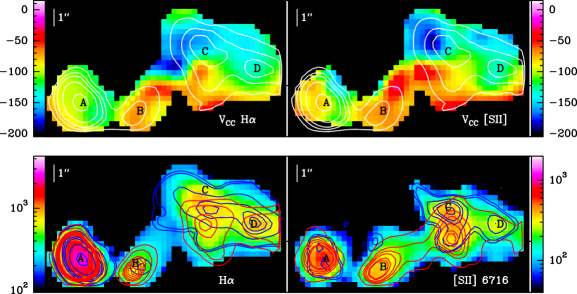
Figure 4: Lower panels: Integrated intensity maps obtained by integrating the signal within all the H$\alpha$ (left) and [S ii] $\lambda$ 6716 Å (right) line profiles (zero-order intensity momenta). For each of the panels, the red contours correspond to the emission intensity obtained by integrating the signal for $V_{\mathrm{LSR}}$ $\geq$ –90 km s^-1(LVC) and the blue contours, to the emission intensity for $V_{\mathrm{LSR}}$ $\leq$ –90 km s^-1. Upper panels: Radial velocity field obtained from cross-correlation in the H$\alpha$+[N ii] range (left), and [S ii] 6716, 6731 Å ranges (right). The velocity scale is in km s^-1. White contours, as in Fig. 3.

Radial velocity maps were first derived from the line centroids of a single-Gaussian fit to the H$\alpha$ and [S ii] emission line profiles. However, a careful inspection of the spectra extracted at several positions on HH 223 reveals that the emission lines display broad, asymmetric and even double-peaked shapes, suggesting that at least two kinematic components are contributing to the line profile at these positions. Hence, we also derived the radial velocities by applying the cross-correlation technique through the XCORR routine of the DIPSO package. Ideally, the template must be a high-S/N spectrum, with a resolution similar to or better than the target spectrum. Unfortunately, we lack such an ideal template, and we adopted as template the spectrum extracted at the peak of the brightest knot (knot A), which seems to have symmetric line profiles. The velocity maps derived from these two methods are in good agreement and show a rather complex pattern in the observed lines. Figure 4 (upper panel) shows the maps of the radial velocity field for the H$\alpha$ and [S ii] emissions. In order to estimate the radial-velocity uncertainties, we compared the values derived from the two techniques (single-Gaussian fit to the profiles, and cross-correlation) giving a mean difference in radial velocities of 2$\pm$6 km s^-1. The largest differences between the radial velocity maps derived from the two techniques are found at positions with clear double-peaked line profiles.

The derived velocities are highly blueshifted, with values ranging from –180 to –60 km s^-1. The velocity field shows a rather complex pattern. In spite of that, some trends can be observed in the spatial distribution of the velocities: the lowest (absolute) velocity values, ranging from –80 to –60 km s^-1, come from the low-brightness emission that connects knot A with knots C and D, and from a shell at the south of the knots A to D intensity peaks. The highest (absolute) velocity values, ranging from –180 to –150 km s^-1, come from a region at the northeast of knot C intensity peak. Finally, we derived velocities ranging from $\simeq$ –130 to $\simeq$ –90 km s^-1 for the emissions arising around the knot A, C and D intensity peaks.

The line profile shapes of most of the spectra suggested a contribution to the emission from two kinematic components. To explore this possibility, we built two chanel maps, by considering two ranges for the velocity: the higher blueshifted component (HVC), for $V_{\mathrm{LSR}}$$\leq$ –90km s^-1, and the lower blueshifted component (LVC), for $V_{\mathrm{LSR}}$$\geq$ –90km s^-1. Then, we obtained the emission maps of the LVC and HVC, for the H$\alpha$ and [S ii]  lines, by integrating the signal within the corresponding velocity range. Figure 4 (lower panels) displays the spatial distribution of the two velocity components. Contours for the HVC (blue) and LVC (red) have been overlapped onto the integrated emission (zero-order intensity moment). All the knots have emission from both kinematic components. However, the spatial distribution of these two velocity components does not fully coincide in H$\alpha$ neither in [S ii] lines. The most remarkable differences appear for knots B and C, where the peak intensity positions of the HVC and LVC appear shifted. We measured offset values of 0.9 and 1.5 arcsec in H$\alpha$ and [S ii] respectively for knot C, and offsets of 0.7 and 1.5 arcsec for knot B. These offset values are reliable, according to the spatial resolution of the data.

Clear doubled-peaked emission lines were only found in a set of spectra arising from the bright nebula at several positions south of the knot A and B intensity peak, and from the region covering knot C (see Fig. 5, upper panel). We additionally performed a line-profile decomposition to reproduce the H$\alpha$+[N ii] 6548,6584 Å, and the [S ii] 6716,6731 Å line profiles of the spectra coming from these regions. The line-profile decomposition was obtained from a model including two Gaussian components. The fitting was performed using the DIPSO package of STARLINK, and the results are shown in Fig. 5. The two velocity components derived in this way appear blueshifted. For the higher blueshifted component (HVC), velocities ranging from –180 km s^-1 to –130 km s^-1 are obtained. The velocities derived for the lower blueshifted component (LVC) range from –80 km s^-1 to –40 km s^-1.

Unfortunately, there are few spectra where a reliable line-profile decomposition can be obtained, not allowing us to infer whether the two kinematic components are tracing emission with different physical conditions, having thus different origin or not. However, a trend is found that consists in the HVC having a higher degree of excitation (with [S ii]/H$\alpha$ ratios $\leq$ 1) and lower electron density ($n_{\mathrm{e}}$ ranging from $\simeq$ 200 to 800 cm^-3) than the LVC, which is less excited ([S ii]/H$\alpha$ $\geq$ 1) and denser ($n_{\mathrm{e}}$ ranging from 1500 to 6000 cm^-3). It should be mentioned that a similar behaviour for the excitation and electron density have been detected in jets emerging from Class 0/I sources and in microjets from TTauri stars (see, e. g. Hamman, 1994; Hirt, Mundt & Solf, 1997; García-López et al., 2008; García-López et al., 2010). From the analysis of the double-peaked line profiles, these authors found that the emission from the LVC usually presents higher electron density and lower excitation than the emission coming from the HVC. In most cases, the LVC is spatially more compact, and is detected only up at a few arcsec near the exciting jet source, around the jet launching region, being related to the launching mechanisms. This scenario does not fit our case, because the knots mapped in HH 223 are far away ($\sim$ 0.1 pc) from the outflow exciting source. Two-peaked line profiles have also been observed in the brighter knots of HH 32 (see e. g. Solf, Böhm & Raga, 1986, and , 2004). In this case, the profiles have been interpreted as originated from the emission of bow-shocks. However, at the light of the 3D kinematics derived from our observations, it is not clear that the bow-shock interpretation could work so well in HH 223 (see later). In other cases (e. g. HH 34 and HH 46-47) the origin of the LVC at larger distances from the source is attributed to the gas entrained and accelerated by the high-velocity outflow. This might be a plausible explanation for the origin of the LVC emission in HH 223. However, a more close similarity in the spatial distribution of the two velocity components should be expected in this case. Alternatively, the detection of two velocity components that also differ in their excitation has been attributed to episodic velocity variations in the outflow (e. g. HH 151, Movsessian, Magakian & Moiseev, 2012). This possibility (i. e. episodic mass-ejection events with variable velocity and direction, as can be expected when the exciting outflow source belongs to a multiple system) might be a more plausible explanation for the origin of the LVC and HVC emissions in HH 223.

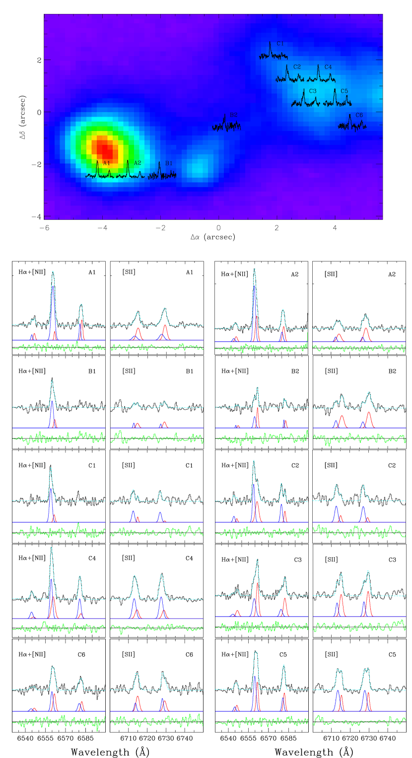
Figure 5: Top: Location of the spectra where double-peaked emission lines are detected, overplotted onto the H$\alpha$ narrow-band image of HH 223 (same as Fig.1). Bottom: Observed spectra (black, continuous) and fits (blue, dashed) obtained from the model of two Gaussian components applied to the H$\alpha$+[N ii] 6548,6584 Å (left) and [S ii] 6716,6731 Å (right). The two individual components are shown below in each panel. The same colour (red and blue) indicates the same component for each line. Residual obtained subtracting the fit from the observed spectra are plotted in green. Labels in the right corner of each plot indicate the corresponding spectra plotted in the top panel of this figure.

3.3 Long-slit vs. IFS

In spite of the comparisons not being fully straightforward, one of the goals of these observations was to check whether the results derived from IFS data are fully consistent with the ones obtained from the long-slit sampling. Apparently some discrepancies in the spatial behaviour of the velocity appeared when IFS results (this work) are compared with those obtained from long-slit observations of López et al. (2009). For example, as can be seen from Fig. 4, low negative velocity values are found associated with knot B emission ($V_{\mathrm{LSR}}$$\simeq$ –70 km s^-1around the H$\alpha$ knot intensity peak), and high negative velocity values appear associated with knot C (with $V_{\mathrm{LSR}}$$\simeq$ –150 km s^-1 around the H$\alpha$ knot intensity peak), reaching even higher negative values ($V_{\mathrm{LSR}}$$\leq$ –180 km s^-1) at positions north to the knot C intensity peak. In contrast, we found velocities of $\simeq$ –130 km s^-1and $\simeq$ –70 km s^-1 at positions sampled from long-slit spectroscopy through knots B and C, respectively. However, we concluded that, in this case, the differences found between the results from IFS and long-slit observations mainly arise as a result of an incomplete sampling of the highly complex kinematics of HH 223.

Table 1: Proper motions ($V_{\mathrm{T}}$)¹ and full spatial velocities ($V_{\mathrm{tot}}$) of HH 223 knots

Knot	$V_{\mathrm{T}}$	PA	$V_{\mathrm{tot}}$	$\phi$
	(km s-1)	(degrees)	(km s-1)	(degrees)
A	$36.4\pm 2.2$	$144\pm 6$2	$107.6\pm 5.0$	$70\pm 5\phantom{1}$
B	$49.2\pm 3.9$	$106\pm 3$2	$84.4\phantom{1}\pm 6.4$	$54\pm 6\phantom{1}$
C	1$3.0\pm 6.5$	0$52\phantom{1}\pm 104$	0$120.7\pm 8.3$1	$89\pm 19$
D	$15.0\pm 2.4$	$99\phantom{1}\pm 6$2	0$120.0\pm 8.7$1	$89\pm 10$
E	$60.3\pm 2.7$	$87\phantom{1}\pm 1\phantom{2}$
F1	$40.8\pm 3.9$	1$80\phantom{1}\pm 11\phantom{2}$
F2	$64.3\pm 2.5$	$91\phantom{1}\pm 6$2
F3	1$7.5\pm 4.2$	0$194\pm 57$1

• ¹ A distance of 300 pc has been adopted. The uncertainty in the L723 distance was not taken into account for derive the errors in proper motions quoted in the table.

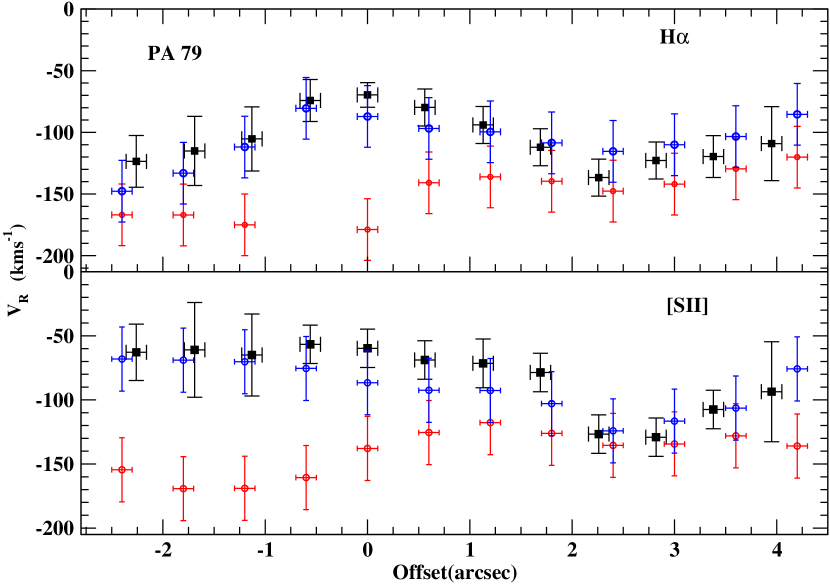
Figure 6: Comparison of radial velocities derived from long-slit spectra (black) and from IFS spectra, obtained through simulated slits of 1 arcsec width positioned at P.A. 79^∘: crossing the knot C intensity peak (blue); the same, but 2 arcsec north of it (red). Offsets are relative to the knot C intensity peak.

To make more meaningful the comparisons, we proceeded to simulate long-slit spectra from the IFS data with a close similar sampling as in long-slit observations. First, we built a grid of 0.3 arcsec spacing; then, we interpolated the signal to extract one-dimensional spectra at positions intersected by two simulated slits of 1 arcsec width. The simulated slits were positioned crossing the peak intensities of knots A and C, at position angles (PA) 73^∘ and 79^∘ respectively. We derived the radial velocities (from the centroids) and line ratios (from the fluxes) of the HH 223 emission within the simulated slits from Gaussian fits to the lines of these extracted spectra. Figure 6 shows the radial velocities derived from the centroids of the H$\alpha$ and [S ii] 6716 Å emission lines (blue). The corresponding radial velocities derived from long-slit spectra are represented by the black dots. Figure 7 shows the [N ii]/H$\alpha$ and [S ii]/H$\alpha$ line ratios (both are tracers of the excitation conditions) and the electron density, $n_{\mathrm{e}}$, from the [S ii] 6716/6731 line ratio, obtained from the spectra along the simulated slit (blue) and the corresponding values from long-slit observations (black). As can be seen from these figures, both the kinematics and the physical conditions of the emission intersected by the simulated slit are compatible with those found from the long-slit sampling. In contrast, some discrepancies appear when velocities derived from long-slit are compared with those obtained from IFS spectra through the simulated slit, but displaced, in parallel, $\sim$ 2 arcsec north to the one crossing the knots peaks (red dots in Fig. 6). This test reveals the importance of obtaining 2D maps covering the full spatial extension of the emission, instead of doing 1D long-slit sampling, mostly in the cases where the kinematics and physical conditions of the emission show such as complex pattern, as in HH 223.

Table 2: $V_{\mathrm{LSR}}$ (km s^-1) line centroids¹ of the HH 223 knots from IFS data.

Knot	[N ii]	H$\alpha$	[N ii]	[S ii]	[S ii]	Average	rms
	6548 Å		6583 Å	6716 Å	6731 Å
A	1$-88.3$	$-101.3$	1$-86.9$	1$-86.1$	1$-85.4$	1$-89.6$	6.61
B	1$-78.7$	1$-68.6$	1$-77.3$	1$-67.8$	1$-67.2$	1$-71.9$	5.61
C	1$-94.2$	$-120.7$	1$-91.9$	$-103.0$	$-102.3$	$-102.5$	11.3
D	$-116.7$	$-124.3$	$-115.2$	$-120.7$	$-120.0$	$-119.4$	3.61

• ¹ Typical value of the error is 5 km s^-1

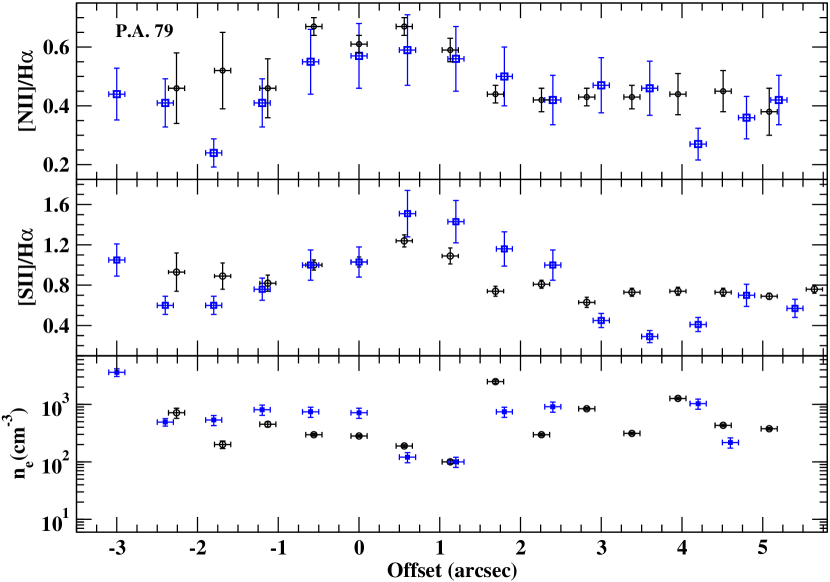
Figure 7: Comparison of line ratios obtained from long-slit spectra (black) and from IFS spectra obtained through simulated slits of 1 arcsec width and positioned at P.A. 79^∘ crossing the knot C intensity peak (blue).

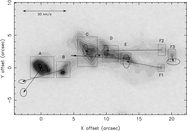
Figure 8: CCD H$\alpha$ image of HH 223 from the last epoch (2009). Arrows indicate the proper motion of the knot. The ellipse at the end of the arrow indicates the uncertainty in the components of the velocity vector. Boxes include the regions used for calculation of the knot proper motion. The same boxes have been taken to evaluate the representative radial velocity of the knot used to derived the full spatial velocity (see text).

4 3D kinematics

The HH 223 emission shows an appreciable undulating morphology. To better characterize the velocity field of the emission, we searched for the full spatial velocity and the inclination angle in the plane of the sky for the HH 223 knots covered by the IFS observations. With this aim, we combined the proper motions of HH 223, derived for the first time in this work, and radial velocities, derived from the current IFS data.

4.1 Proper motion determination

The tangential velocity, $V_{\mathrm{T}}$, of the knots was derived from their proper motions, using three narrow-band H$\alpha$ images of the L723 field, obtained at the NOT telescope, with a time baseline of 5 years (see §2.2). These images were converted onto a common reference system using the position of ten common field stars, well distributed around HH 223, to register the images. The GEOMAP and GEOTRAN task of IRAF were applied to perform a linear transformation with six free parameters that take into account relative translation, rotation and magnification among the frames. The procedure to calculate the proper motions from multiepoch images has been described in detail by López et al. (2005) and (2007) for the cases of HH 110 and HH 30, respectively. In short, it consists of defining boxes in each frame that include the emission from the individual knot; then, to compute the two-dimensional cross-correlation function of the emission for the two pairs of frames (the 2004 first epoch image and each of the other two epoch images), and to determine the displacements in $x$ and $y$ coordinates through a parabolic fit to the peak of the cross-correlation function; finally, to perform a linear regression fit to the displacements of the $x$ and $y$ coordinates as a function of the epoch offset, from the first epoch (2004). We derived the proper motion velocity ($V_{\mathrm{T}}$) and the position angle (PA) for each knot from the slope of the fitted straight line (and its uncertainty) . The results are displayed in Fig. 8, and their values, in columns 2 and 3 of Table 1. The errors include the uncertainty in the position of the correlation peak (derived as explained in López et al., 2005), and the error in the alignment of the frames.

4.2 Full spatial velocities

The IFS data have revealed a complex kinematic structure for the HH 223 emission in such a way that radial velocity values of the knots show variations depending on the parcel of the knot emission sampled within the slit (see e. g. Fig. 6). Note that the emission of each knot in HH 223 extends over several arcsec, both in the $x$ and $y$ coordinates (see e. g. Fig. 1), being thus improperly sampled by a single long-slit ponting. Since IFS allows us to achieve a more complete sampling of the kinematics, we can assign to each knot a representative radial velocity coming from the emission enclosed in the same box that we defined to measure the knot proper motion. The radial velocity derived in this way will be used to calculate the full spatial velocity of the knot. We then defined the aperture enclosing each of the boxes A to D (see Fig. 8), and compute the line profiles by integrating the signal over the fibers inside the aperture. We then determined the radial velocity from a Gaussian fit to the emission lines (see Table 2).

The full spatial velocity ($V_{\mathrm{tot}}$) and the angle $\phi$ between the knot motion and the plane of the sky (with positive values of $\phi$ towards the observer) are then derived from the H$\alpha$ radial velocity (obtained from IFS data) and the proper motions (obtained from H$\alpha$ CCD narrow-band images). The results are given in columns 3 and 4 of Table 1. Unfortunately, we were only able to obtain $V_{\mathrm{T}}$ and $\phi$ for the four HH 223 knots covered by the single IFS pointing. We found that these knots present high full spatial velocities ($\geq$ 100 km s^-1) and move in a direction close perpendicular to the plane of the sky. However, the data suggest that there is some change in the jet inclination, which increases going from the southern knot B (also with the lowest full velocity) to the northern knots C and D.

Apparently, the 3D kinematics of HH 223 (i. e. the radial velocity structure and the proper motions) shows close similarities with HH 32 (see, e. g. Solf, Böhm & Raga, 1986, and Curiel et al., 1997): both HHs are oriented close to the line of sight and present two-peaked line profiles (note however that in the case of HH 223, the two-peaked line profiles are not detected at the brightest knot, HH 223-A). Raga et al. (2004) modeled the HH 32 emission as a broken-up, large scale bow-shock with several condensations. The bow-shock interpretation succeeded in deriving the bow-shock properties, like the bow-shock velocity ($V_{\mathrm{bs}}$) and the orientation angle of the outflow in the plane of the sky ($\phi$), from the components of the proper motion velocity parallel and perpendicular to the projected outflow axis (Raga et al., 1997). However, in spite of the similarities between the HH 32 and 223 structures, the bow-shock interpretation seems not work so well for HH 223. Assuming a projected outflow axis at P.A. of 110–115$\degr$ (the P.A. of the east-west CO bipolar outflow, see e. g. Moriarty-Schieven & Snell, 1989; Lee et al., 2002) and from the measured proper motions, the bow-shock model would give a low shock velocity ($V_{\mathrm{bs}}$$\leq$ 25 km s^-1) and an orientation outflow angle close to the plane of the sky ($\phi~{}\leq$ 30$\degr$), which is far from the direction derived using the observed radial and tangential velocity components presented here, even taking into account the uncertainty of the proper motions due to the uncertainty in the distance to L723.

5 SUMMARY AND CONCLUSIONS

We carried out a single-pointing IFS observation of HH 223, the optical counterpart of a larger scale ($\sim$ 5.5 arcmin, $\sim$ 0.5 pc at a distance of 300 pc) H₂ outflow, driven by the protostellar source VLA 2A, in L723. Because of its peculiar and poorly collimated morphology, this target was selected for the backup list of a science verification program of a new INTEGRAL equalized fiber bundle. IFS observations have revealed to be the best choice to achieve a reliable mapping of the whole spatial emission of such chaotic outflows. The results derived from IFS data were compared with previous long-slit and CCD narrow-band images looking for consistency. Unfortunately, because of the observing time available for our target in the backup program, it was not possible to acquire an additional pointing to cover the fainter HH 223 knots E to F. New results derived from our analysis of the IFS data are summarized below:

• The morphology of the HH 223 emission shown by the line intensity maps built from the IFS data is in good agreement with the morphology found in the narrow-band images. One advantage to get line intensity maps from IFS data is the capability of mapping separately the emission coming from lines that usually are included into the same narrow-band filter (e. g. H$\alpha$ and [N ii] 6584 Å). We obtained in this work a map for each of the emission lines that revealed the close similarity between the [S ii] and [N ii] emissions and some differences between the spatial brightness distribution of the neutral (H$\alpha$) and ionized ([N ii] and [S ii]) gas.

• We traced the spatial distribution of the excitation and the electron density from line-ratio maps. These maps revealed the complexity of the spatial structure of the physical conditions. It makes once again IFS mapping highly appropriate to properly reveal physical conditions of the emission, instead of derive them from a partial sampling obtained from long-slit data. As a general trend, the [S ii]/H$\alpha$ and [N ii]/H$\alpha$ ratios are consistent with the emission arising from shocks with an intermediate/high degree of excitation. A relevant result concerning the electron density is the inhomogeneities found through the emission (both, through the knots and through the low-brightness nebula), which suggests a clumpy structure that cannot be well resolved with the current IFS spatial resolution.

• The radial velocity field has been derived, first from the line centroid of a single-Gaussian fitting to the lines profile and, in addition, from the cross-correlation technique. Results found from both procedures are fully consistent. The velocities are highly blueshifted, ranging from –180 to –60 km s^-1. They present a complex pattern in the spatial distribution, with some trend that consists of the more negative (blueshifted) values increasing moving from southeast to northwest.

• The spectra extracted at several positions show clear double-peaked line profiles. We were able to reproduce the line profiles for these spectra using a model that included two blueshifted kinematic components. In addition, some trend is found that consists of the HVC (velocity ranging from –180 to –130 km s^-1) being more excited and rarefied than the LVC (velocity ranging from –80 to –40 km s^-1). The two velocity components, having quite different physical properties and spatial distributions, can be indicative of a variability in the properties of the outflow ejection (e. g. episodic mass ejection events having some different velocity and direction). This can be expected when the outflow source is a binary or a multiple system, as was proposed by Carrasco-González et al. (2008).

• To search for the reliability of two kinematic components through all the emission mapped, we performed chanel maps both, in H$\alpha$ and in [S ii], for two velocity ranges: a HVC (for $V_{\mathrm{LSR}}$ $\leq$ –90 km s^-1), and a LVC (for $V_{\mathrm{LSR}}$ $\geq$ –90 km s^-1). We found differences between the spatial distributions of the HCV and LVC. The most remarkable differences are found in knots C and B, where we measured offset values from 0.7 to 1.5 arcsec between the positions of their LVC and HVC emission peaks. Taking into account the spatial resolution of our data, these offsets are reliable.

• We checked the results on the kinematics and physical conditions derived from long-slit data with those derived from IFS. With this aim, we simulated a long-slit and extracted spectra with a similar sampling along this slit, positioned as in long-slit data acquisition. This test lead us to conclude that the physical conditions and kinematics derived from long-slit spectra are in good agreement with those derived from IFS spectra that were extracted at the same positions. In contrast, we found that appreciable differences could arise when long-slit data are compared with IFS spectra that were extracted along slits displaced few arcsec from the nominal long-slit position. This test reinforces again the IFS mode to get a more accurate picture of such as complex outflows.

• Comparing the spatial distribution of the gas excitation (Fig.3) and kinematics (Fig.4), we can observe a similar structure of the maps, which illustrates a relationship between the degree of gas excitation and the velocity. In particular, the regions having a higher degree of gas excitation (around knots C and A) coincide with the ones were the velocity values are more negative, while emission of lower excitation (located north of knot B and south of knots C and D) also displays less negative velocity values. We cannot appreciate a similar relationship when the maps of the electron density and velocity are compared, probably because the spatial distribution of the electron density has a pattern more complex than the excitation

• We calculated the full spatial velocity and the inclination angle of its motion in the plane of the sky for the knots mapped with IFS. From proper motion measurements, using multiepoch narrow-band images, and radial velocities, derived from IFS, we found that the knots have full spatial velocities higher than 100 km s^-1and move close to the line of sight. Furthermore, a change in the jet inclination is also outlined.

References

- (1) Allen, C. W. 1973, Astrophysical Quantities, 3rd Ed. (London:Athlone).
- (2) Anglada, G., Estalella, R., Rodríguez, L.F.,Torrelles, J.M., López, R., Cantó J. 1991, ApJ, 376, 615.
- (3) Anglada, G., López, R., Estalella, R., Masegosa, J., Riera, A, & Raga, A.C. 2007, AJ, 132, 2799.
- Arribas et al. (1998) Arribas, S., et al. 1998, Proc. SPIE, 3355, 821.
- (5) Beck, T.L., Riera, A., Raga, A.C. & Aspin, C. 2004, AJ, 127, 408.
- Bingham et al. (1996) Bingham, R.G, Gellatly, D.W., Jenkins, C.R., & Worswick, S.P. 1994, Proc. SPIE, 2198, 56.
- Cantó (1981) Cantó, J. 1981 in Investigating the Universe, ed., F. Kahn (Dordretch:Reidel), 95.
- Carrasco-González et al. (2008) Carrasco-González, C., Anglada, G., Rodríguez, L.F.,Torrelles, J.M., Osorio, M., Girart, J.M. 2008, ApJ, 676, 1073.
- Curiel et al. (1997) Curiel, S., Raga, A.C., Raymond, J., Noriega-Crespo, A., & Cantó, J. 1997, AJ, 114, 2736.
- García-López et al. (2008) García-López, R., Nisini, B., Giannini, T., Eislöffel, J., Bacciotti, F., & Podio, L. 2008, A&A, 487, 1019.
- García-López et al. (2010) García-López, R., Nisini, B., Eislöffel, J., Giannini, T., Bacciotti, F., & Podio, L. 2010, A&A, 511, A5.
- García-Lorenzo et al. (2002) García-Lorenzo, B., Acosta-Pulido, J.A., & Megías-Fernández, E. 2002, in ASP Conf. Ser. 282, Galaxies: The Third Dimension, ed. M. Rosado, L. Binette, & L. Arias (San Francisco: ASP), 501.
- García-Lorenzo et al. (2005) García-Lorenzo, B., Sánchez, S.F., Mediavilla, E., González-Serrano, J.I., & Christensen, H. 2005, ApJ, 621, 146.
- Goldsmith et al. (1984) Goldsmith, P. F., Snell, R. L., Hemeon-Heyer, M., & Langer, W. D. 1984, ApJ, 286, 599.
- Hamman (1994) Hamman, F. 1994, ApJS, 93, 485.
- Hirt, Mundt & Solf (1997) Hirt, G.A., Mundt, R., & Solf, J. 1997, A&AS, 126, 437.
- Lee et al. (2002) Lee, C.F., Mundy, L.G., Stone, J.M., & Ostriker, E.C. 2002, ApJ, 576, 294.
- López et al. (2005) López, R., Estalella, R., Raga, A.C., Riera, A., Reipurth, B., & Heathcote, S.R. 2005, A&A, 432, 567.
- López et al. (2006) López, R., Estalella, R., Gómez, G., & Riera, A. 2006, A&A, 454, 233.
- López et al. (2008) López, R., García-Lorenzo, B., Sánchez, S.F., Gómez, G., Estalella, R., & Riera, A. 2008, MNRAS, 391, 1107.
- López et al. (2009) López, R., Estalella, R., Gómez, G., Riera, A., & Carrasco-González, C. 2009, A&A, 498, 761.
- López et al. (2010a) López, R., Acosta-Pulido, J. A., Estalella, R., Gómez, G. & Carrasco-González, C. 2010a, A&A, 523, A16.
- López et al. (2010b) López, R., García-Lorenzo, B., Sánchez, S.F., Gómez, G., Estalella, R., & Riera, A. 2010b, MNRAS, 406, 2193.
- Moriarty-Schieven & Snell (1989) Moriarty-Schieven, G.H. & Snell, R. 1989, ApJ, 338, 952.
- Movsessian, Magakian & Moiseev (2012) Movsessian, T.A., Magakian, T.Y., & Moiseev, A.V. 2012, astro-ph 1203.4074.
- Raga et al. (1996) Raga, A.C., Böhm, K.-H. & Cantó, J. 1996, RevMexAA, 32,161.
- Raga et al. (1997) Raga, A.C., Cantó, J., Curiel, S., Noriega-Crespo, A. & , Raymond, J.C. 1997, RevMexAA, 33,157.
- Raga et al. (2004) Raga, A.C., Riera, A., Masciadri, E., Beck, T.L., Böhm, K.-H. & Binette, L. 2004, AJ, 127, 1081.
- Reipurth (1994) Reipurth, B., 1994, A general catalogue of Herbig-Haro objects, Electronic version 1994-1.
- Solf, Böhm & Raga (1986) Solf, J., Böhm, K.-H. & Raga, A.C. 1986, ApJ, 305, 795.
- Torrelles et al. (1986) Torrelles, J.M., Ho, P.T.P, Moran, J.M., Rodríguez, L.F., Cantó J. 1986, ApJ, 307, 787.