Bosonic Cascade Laser

Abstract

We propose a concept of a quantum cascade laser based on transitions of bosonic quasiparticles (excitons and exciton-polaritons) in a parabolic potential trap in a semiconductor microcavity. This laser would emit terahertz radiation due to bosonic stimulation of excitonic transitions. Dynamics of a bosonic cascade is strongly different from the dynamics of a conventional fermionic cascade laser. We show that populations of excitonic ladders are parity-dependent and quantized if the laser operates without an external terahertz cavity.

Quantum cascade lasers (QCLs) are based on subsequent intersubband transitions of electrons or holes in a Wannier-Stark ladder formed in a semiconductor superlattice subject to an external electric field Kazarinov1971 ; Faist1994 ; Normand2007 . Emitted terahertz (THz) photons are polarized perpendicularly to the plane of the structure and propagate in-plane (which is referred to as wave-guiding or horizontal geometry). QCLs differ from conventional lasers as they do not require inversion of electronic population for every particular transition. Still, this is a fermionic laser, where the quasiparticles emitting light obey Fermi statistics. Recently, several proposals for bosonic THz lasers based on exciton-polaritons have been published Kavokin2010 ; Savenko2011 . These sources are expected to generate THz light beams propagating in the normal-to-plane direction (vertically) without external THz cavities Kavokin2012 . The emitted radiation is stimulated by the final state (exciton-polariton) occupation, which is a purely bosonic effect.

Here we propose a concept of a bosonic cascade laser, which combines the advantages of QCL (emission of multiple THz photons for each injected electron) and exciton-polariton lasers (no need for a THz cavity, low threshold). We consider an exciton cascade formed by equidistant energy levels of excitons confined in a parabolic trap in a semiconductor microcavity. Parabolic traps for exciton-polaritons have been experimentally demonstrated, and an equidistant spectrum of laterally confined exciton-polariton states has been observed. There are several ways to realize such traps including specially designed pillar microcavities Bajoni2007 , strain induced Snoke2007 and optically induced traps Amo2010 ; Wertz2010 ; Tosi2012 . A particularly promising variation of these designs would be a microcavity with a large parabolic quantum well embedded. We consider the weak coupling regime where the optical mode is resonant with the m^th exciton level to allow efficient pumping. The other energy levels of the confined excitons would be uncoupled to the cavity mode, forming a dark cascade ideal for a high quantum efficiency device due to the long radiative lifetime. This device would emit radiation polarized in the direction normal to the quantum well plane and propagating in the cavity plane in the wave-guiding regime. In this Letter we formulate a kinetic theory of bosonic cascade lasers and calculate the matrix elements of terahertz transitions in realistic parabolic traps.

The occupation numbers of exciton quantum confined states and the THz optical mode in our cascade laser can be found from the following set of kinetic equations ($0$ is the state with the lowest energy, $m$ is the state with the highest energy, which is resonantly pumped):

$$\frac{\mathrm{d}N_{m}}{\mathrm{d}t} =P-\frac{N_{m}}{\tau}-WN_{m}(N_{m-1}+1)$$

$$\hskip 56.9055pt+W^{\prime}N_{m-1}(N_{m}+1),$$ (1)

$$\frac{\mathrm{d}N_{k}}{\mathrm{d}t} =-\frac{N_{k}}{\tau}+W\left[N_{k+1}(N_{k}+1)-N_{k}(N_{k-1}+1)\right]$$

$$\hskip 28.45274pt+W^{\prime}\left[N_{k-1}(N_{k}+1)-N_{k}(N_{k+1}+1)\right]$$

$$\hskip 71.13188pt\forall\quad 2\leq k\leq m-1,$$ (2)

$$\frac{\mathrm{d}N_{0}}{\mathrm{d}t} =-\frac{N_{0}}{\tau}+WN_{1}(N_{0}+1)-W^{\prime}N_{0}(N_{1}+1),$$ (3)

$$\frac{dn_{\mathrm{THz}}}{dt} =-\frac{n_{\mathrm{THz}}}{\tau_{\mathrm{THz}}}+W\sum_{1}^{m}N_{k}\left(N_{k-1}+1\right)$$

$$\hskip 56.9055pt-W^{\prime}\sum_{1}^{m}N_{k-1}\left(N_{k}+1\right).$$ (4)

Here $W=W_{0}(n_{\mathrm{THz}}+1)$ is the THz emission and $W^{\prime}=W_{0}n_{\mathrm{THz}}$ is the THz absorption rate, $n_{THz}$ is the THz mode occupation, and $\tau_{\mathrm{THz}}$ is the THz mode lifetime. We assume that the matrix element of THz transition is non-zero only for neighbouring stairs of the cascade and that it is the same for all neighbouring pairs. This simplifying assumption allows for the analytical solution of Eqs. (1) – (3). It can be easily relaxed in the numerical calculation, accounting for the specific conditions of particular experimental systems.

We first consider the case where there is no THz cavity, and assume that THz photons leave the system immediately such that $n_{\mathrm{THz}}=0$. The solid curves in Fig. 1 show the dependence of the mode occupations on the pump power in this case, which were calculated by numerical solution of equations (1) – (3) for the steady state. For increasing pump power we see that the modes become occupied one-by-one and a series of steps appears, each corresponding to the occupation of an additional mode. In the limit, $W_{0}\tau\ll 1$, the position of the steps is given by $P/W_{0}=n^{2}/(W_{0}\tau)^{2}$ where $n$ is a half-integer. For high pump powers, where all modes are occupied two different behaviours of the modes can be identified: 0th, 2nd, 4th etc modes continue to increase their occupation with increasing pump power, while 1st, 3rd, 5th etc modes have a limited occupation. This effect persists independently of whether an even or odd number of modes is considered in the system.

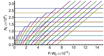
Figure 1: (color online) Dependence of the mode occupations in the absence of a THz cavity on pump intensity, calculated numerically from the kinetic Eqs. (1) – (3) (solid curves) and analytically from Eqs. (5), (6) and (7) (dashed curves). The vertical gray lines correspond to the step locations given by $P/W_{0}=n^{2}/(W_{0}\tau)^{2}$ where $n$ is a half-integer. Parameters: $W_{0}\tau=3\times 10^{-6}$, $m=15$, $n_{\mathrm{THz}}=0$.

Qualitatively, our results can be understood as follows. Every mode in the chain experiences both a gain and a loss. The last mode in the chain is unique since it only experiences loss due to the finite lifetime rather than THz emission. Since it experiences loss only due to the lifetime, we can expect that the last mode is strongly occupied in the limit of high pump power. This means that the second-to-last mode experiences a strong loss due to stimulated scattering to a highly occupied state. Thus the second-to-last mode has a much smaller occupation. The third-to-last mode then experiences only a small loss due to stimulated scattering and so can again have a large occupation. The series repeats such that alternate modes have high and low intensity, with the highly occupied modes introducing a fast loss rate that limits the occupation of low intensity modes.

Quantitatively, Eqs. (1) – (3) can be solved analytically in the steady state, where $\sum_{k}N_{k}=P\tau$, under the assumption that $W_{0}\tau\ll 1$, $N_{m}\gg 1$ and $n_{\mathrm{THz}}=0$. In this regime, $N_{0}$ depends linearly on the pump intensity:

$$N_{0}=\frac{P\tau}{\lceil(m+1)/2\rceil}-\frac{1}{W_{0}\tau}\lceil\frac{m}{2}\rceil,$$ (5)

where $\lceil n\rceil$ denotes rounding up to the nearest integer. Our approximation makes sense when $N_{0}$ is positive, i.e., when $P\tau>m^{2}/(2W_{0}\tau)^{2}$. The populations of modes with even index also depend linearly on the pump intensity:

$$N_{2l}=N_{0}+\frac{l}{W_{0}\tau}\hskip 14.22636pt\forall\hskip 14.22636pt0\leq l\leq\lceil(m-1)/2\rceil$$ (6)

The populations of the odd modes are:

$$N_{2l-1}=\frac{l}{W_{0}\tau}\hskip 14.22636pt\forall\hskip 14.22636pt0\leq l\leq\lceil m/2\rceil$$ (7)

Results from Eqs. (5), (6) and (7) are compared to the numerical results in Fig. 1. It is also possible to write an equation for the THz emission rate:

$$\frac{dn_{\mathrm{THz}}}{dt} =W_{0}\sum_{1}^{m}N_{k}\left(N_{k-1}+1\right)$$ (8)

$$\approx\frac{m^{2}+1}{4\tau}\left[N_{0}-\frac{m-1/2}{3W_{0}\tau}\right].$$ (9)

Results from Eq. (9) are compared to numerical calculation of the THz emission rate in Fig. (2)a. For high pump powers, the rate increases linearly with the pump power. This represents a limit to the quantum efficiency of THz emission, which is given by the THz emission rate divided by the pump rate, $P$, and plotted in Fig. 2b. While the presence of the bosonic cascade allows quantum efficiencies exceeding unity, the quantum efficiency is limited under high pump powers to $\lceil m/2\rceil$, for $W_{0}\tau\ll 1$.

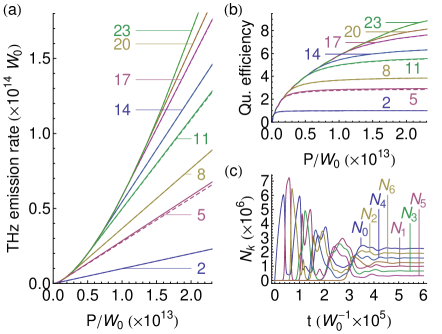
Figure 2: (color online) a) Dependence of the THz emission rate on pump intensity in the absence of a cavity, for different numbers of modes in the chain (values of $m$ are marked on the plot). Solid curves show results from numerical solution of Eqs. (1) – (3); Dashed curves show the results of Eq. (9), valid for high pump powers. b) Dependence of the quantum efficiency on pump intensity (the values of $m$ are the same as in (a)). c) Time dynamics for $m=6$, $P=3\times 10^{12}W$. Parameters: $W_{0}\tau=3\times 10^{-6}$, $n_{\mathrm{THz}}=0$.

Figure 2c shows the typical time dependence of the mode occupations after the pump is switched on (assumed instantaneously). The enhancement of the scattering via stimulated processes allows the system to reach equilibrium in a time less than $1/W_{0}$. The presence of multiple, dynamically changing effective scattering rates causes an initially chaotic dynamics.

In the presence of a THz cavity, macroscopic numbers of THz cavity photons allow further stimulated enhancement of scattering between the modes. In this case, where upward transitions are allowed in addition to downward ones, the steps observed in Fig. 1 are washed out as shown in Fig. 3. In contrast to Fig. 1, all modes continue to increase their population with increasing pump power.

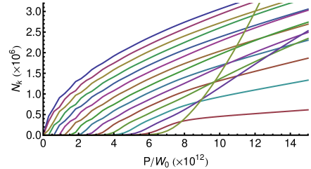
Figure 3: (color online) Same as in Fig. 1 with a THz cavity. $\tau_{THz}=\tau/1000$.

Figure 4a shows the THz emission rate as a function of the THz photon lifetime. For fixed pump intensity, higher THz emission rates are observed than in Fig. 2a.

Figure 4: (color online) a) Dependence of the THz emission rate in the presence of a THz cavity on the THz photon lifetime. Different curves correspond to different pump powers (marked on the plot). b) Dependence of the quantum efficiency on THz photon lifetime for the same pump powers in (a). Parameters: $m=15$, $W_{0}\tau=3\times 10^{-6}$.

Figure 4b shows the dependence of the THz emission quantum efficiency on the THz photon lifetime. Increasing of the THz photon lifetime is able to increase the quantum efficiency, however, not beyond the limit of $m/2$ already observed in the absence of a THz cavity for high pump powers.

Let us now demonstrate the feasibility of THz transitions between the size-quantized levels of excitons in a parabolic quantum well. The two-particle Hamiltonian for an electron and a hole reads

$$\mathcal{H}=-\frac{\hbar^{2}}{2\mu}\frac{\partial^{2}}{\partial\bm{\rho}^{2}}-\frac{e^{2}}{\epsilon\rho}-\frac{\hbar^{2}}{2M}\frac{\partial^{2}}{\partial\bm{R}^{2}}+V(z_{e},z_{h}).$$ (10)

Here $M=m_{e}+m_{h}$, $\mu=m_{e}m_{h}/M$ is the reduced mass of the electron-hole pair, $\bm{\rho}=\bm{r}_{e}-\bm{r}_{h}=(x,y,z)$ is the relative coordinate and $\bm{R}=(m_{e}\bm{r}_{e}+m_{h}\bm{r}_{h})/M=(X,Y,Z)$ is the center of mass wave vector, $\epsilon$ is the background dielectric constant. The quantum well potential $V(z_{e},z_{h})$ is written in form:

$$V(z_{e},z_{h})=A_{e}z_{e}^{2}+A_{h}z_{h}^{2},$$

where constants $A_{e,h}$ denote corresponding stiffness. It is convenient to rewrite $V(z_{e},z_{h})$ as a function of the center of mass $Z$ and relative motion $z$ coordinates with the result $V=V_{0}(Z,z)+V_{1}(Z,z)$, where $V_{0}(Z,z)=(A_{e}+A_{h})Z^{2}+(m_{e}^{2}+m_{h}^{2})z^{2}/M^{2}$ does not mix center of mass and relative motion and

$$V_{1}(Z,z)=\frac{2}{M}(m_{h}A_{e}-m_{e}A_{h})Zz,$$ (11)

mixes internal and center of mass degrees of freedom provided that $m_{h}A_{e}\neq m_{e}A_{h}$.

In what follows it is assumed that the potential is weak enough, hence, in the zeroth approximation center of mass can be quantized independently and $0^{th}$ order wavefunctions have the form:

$$\Psi_{n,m,h}(\bm{r}_{e},\bm{r}_{h})=R_{nlm}(\rho)Y_{lm}(\vartheta,\varphi)F_{h}(Z),$$ (12)

where $F_{h}(Z)$ are the eigenfunctions of the potential $(A_{e}+A_{h})Z^{2}$, $h$ enumerates levels in this harmonic potential, $R_{nlm}(\rho)$ are the 3D-hydrogen-like radial functions and $Y_{lm}(\vartheta,\varphi)$ are (3D) the angular harmonics of relative motion. $n$, $l$ and $m$ are the quantum numbers of relative motion of an electron and a hole. Equation (12) holds if $\hbar\Omega\ll\mathcal{R}$, where $\Omega$ is the eigenfrequency of the center of mass in the parabolic potential, ${M\Omega^{2}}/{2}=A_{e}+A_{h}$, and $\mathcal{R}={\mu e^{4}}/({2\epsilon^{2}\hbar^{2}})$ is the exciton Rydberg.

It is the mixing of the exciton states caused by perturbation Eq. (11) that gives rise to the THz transitions between the neighbouring size-quantized states in a quantum well. Making use of matrix elements of coordinate for harmonic oscillator and for the hydrogen atom Landau1977 ; ll4_eng we obtain for the mixing matrix elements (bra- and ket- denote states as, e.g. $|n,l,m,h\rangle$)

$$\langle 1,0,0,h-1|V_{1}|n,1,0,h\rangle=\langle 1,0,0,h|V_{1}|n,1,0,h-1\rangle=\\ \frac{2}{\sqrt{3}M}(m_{e}A_{e}-m_{h}A_{h})a_{0}f_{n}\sqrt{\frac{h\hbar}{2M\Omega}}\equiv V_{h}(n),$$ (13)

where $a_{0}=\frac{\hbar^{2}\epsilon}{\mu e^{2}}$ is the exciton Bohr radius and

$$f_{n}=\frac{2^{4}(n-1)^{n-5/2}n^{7/2}}{(n+1)^{n+5/2}}.$$

Using first order perturbation theory, the THz transition dipole moment between the neighbouring states is:

$$D_{h}=e\langle\tilde{\Psi}_{h-1}|x|\tilde{\Psi}_{h}\rangle=e\sum_{n,\pm}\frac{V_{h}(n)}{\Delta_{h,\pm}(n)}\frac{f_{n}a_{0}}{\sqrt{3}},$$ (14)

where the wavefunctions of $1s$ exciton states take the form in the leading order in $V_{1}$:

$$\tilde{\Psi}_{1,0,0,h}(\bm{\rho},\bm{R})=R_{100}(\rho)Y_{00}(\vartheta,\varphi)F_{h}(Z)+\\ \sum_{n,\pm}\frac{V_{h}(n)}{\Delta_{h,\pm}(n)}R_{n10}(\rho)Y_{10}(\vartheta,\varphi)F_{h\pm 1}(Z).$$ (15)

Here $\Delta_{h,\pm}(n)=E_{1s}-E_{np}\mp\hbar\Omega\approx E_{1s}-E_{np}$, and $E_{ns}=E_{np}=-{\mathcal{R}}/{n^{2}}$. Estimation according to Eq. (14) shows for $a_{0}=100$ Å, $\mathcal{R}=5$ meV, $\hbar\Omega=1$ meV, $m_{e}=0.1m_{0}$, $m_{h}=0.4m_{0}$ and $A_{e}=A_{h}$ that

$$|D_{h}|=e\sqrt{h}\times 8.3\times 10^{1}~{}\mbox{\AA},$$ (16)

which is comparable with $2p\to 1s$ transition strength. Following Ref. Kavokin2010 , this gives the transition rate for $1$THz emission in the kinetic equations $W_{0}\approx 5500$s^-1 (where we took the refractive index as $3$ corresponding to a GaAs based system). For excitons with lifetime $\sim 500$ps, this gives $W_{0}\tau\approx 3\times 10^{-6}$.

Since the transition rate is proportional to $|D_{h}|^{2}$, Eq. (16) introduces a proportionality between the transition rate and the mode indices, $n$, for the specific case of a parabolic trap with electron-hole mixing. This can be modelled by straightforward modification of the rate Eqs. (1) – (3). While this can distort the steps observed in Fig. 1 as shown in Fig. 5, the behaviour is similar. For $W_{0}\tau\ll 1$ and $m$ even, one can obtain analytically:

$$N_{2k}\approx\frac{1}{W_{0}\tau}-\frac{m\left(1+m-PW_{0}\tau^{2}\right)\Gamma(1/2+k)\Gamma(m/2)}{4W_{0}\tau\Gamma(1+k)\Gamma[(3+m)/2]},$$ (17)

where $k$ is an integer and $\Gamma(n)$ is the Euler gamma function. The other modes of the system all have the same intensity, $N_{2k+1}\approx 1/(W_{0}\tau)$ and the THz emission rate is given by $\left(2P\tau-m/(W_{0}\tau)-N_{0}+N_{m}\right)/(W_{0}\tau)$.

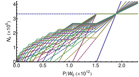
Figure 5: (color online) Same as in Fig. 1 with transition rates proportional to the mode index.

Finally, we note that the waveguiding geometry allows for the increase of the active volume of the laser and, consequently, the output power. Its drawback is a larger size compared to the vertical cavity laser geometry. Lateral polariton traps would allow a more compact size of the device, while the matrix elements of terahertz transitions are believed to be significantly larger in parabolic quantum wells.

In summary, we have proposed the use of a bosonic cascade to implement THz lasing with high quantum efficiency, above unity. Such a device requires a parabolic trapping, which can be arranged in the plane of a semiconductor microcavity via a variety of techniques or using parabolic wide quantum wells. Electron-hole mixing was shown to give rise to non-zero transition matrix elements. A series of steps in the mode occupations of the bosonic cascade was predicted for increasing pump power in the absence of a THz cavity. The quantum efficiency of a device can be improved by increases in the pump power or the use of a THz cavity, however, the quantum efficiency is limited to one-half of the number of modes present.

This work has been supported by the EU IRSES projects “POLAPHEN ”and “POLATER ”. IAS acknowledges the support from Rannis “Center of Excellence in Polaritonics”. MMG was partially supported by RFBR and RF President Grant NSh-5442.2012.2.

References

- (1) R F Kazarinov & R A Suris, Sov. Phys. Semiconductors, 5, 707 (1971).
- (2) J Faist, F Capasso, D L Sivco, C Sirtori, A L Hutchinson, & A Y Cho, Science, 264, 553 (1994).
- (3) E Normand & I Howieson, Laser Focus World, 43, 90 (2007).
- (4) K V Kavokin, M A Kaliteevski, R A Abram, A V Kavokin, S Sharkova, & I A Shelykh, Appl. Phys. Lett. 97, 201111 (2010).
- (5) I G Savenko, I A Shelykh, & M A Kaliteevski, Phys. Rev. Lett., 107, 027401 (2011).
- (6) A V Kavokin, I A Shelykh, T. Taylor & M M Glazov, Phys. Rev. Lett., 108, 197401 (2012).
- (7) D Bajoni, et al., Appl. Phys. Lett., 90, 051107 (2007).
- (8) R Balili, V Hartwell, D Snoke, L Pfeiffer, & K West, Science, 316, 1007 (2007).
- (9) A Amo, et al., Phys. Rev. B, 82, 081301(R) (2010).
- (10) E Wertz, et al., Nature Phys., 6, 860 (2010).
- (11) G Tosi, et al., Nature Phys., 8, 190 (2012).
- (12) L Landau & E Lifshitz, Quantum Mechanics: Non-Relativistic Theory (vol. 3), Butterworth-Heinemann, Oxford (1977).
- (13) V B Berestetskii, L P Pitaevskii, & E M Lifshitz, Quantum Electrodynamics, Second Edition (vol. 4), Butterworth-Heinemann, Oxford, (1999).