Optimising Performance Through Unbalanced Decompositions

Abstract

GS2 is an initial value gyrokinetic simulation code developed to study low-frequency turbulence in magnetized plasma. It is parallelised using MPI with the simulation domain decomposed across tasks. The optimal domain decomposition is non-trivial, and complicated by the differing requirements of the linear and non-linear parts of the calculations.

GS2 users currently choose a data layout, and are guided towards process counts that are efficient for linear calculations. These choices can, however, lead to data decompositions that are relatively inefficient for the non-linear calculations. We have analysed the impact of the data decompositions on the non-linear calculation performance and associated communications. This has helped us to optimise the decomposition algorithm by using unbalanced data layouts for the non-linear calculations whilst maintaining the existing decompositions for the linear calculations. This has completely eliminated communications for parts of the non-linear simulation and improved performance by up to $15\%$ for a representative simulation.

I Introduction

Many scientific simulation techniques, and therefore scientific simulation codes, use spectral methods to solve partial differential equations (PDEs) efficiently. Whilst there are a variety of different techniques to achieve this, the general approach is to use a discrete and finite set of basis functions. This finite set of basis functions allows the PDE to be treated numerically and the solution of the PDE is approximated as a linear combination of the basis functions. Using basis functions with global support is commonly referred to as spectral methods. With periodic boundary conditions, trigonometric functions are a popular choice for the basis. To transfer the numerical solution from the spectral space to the position space one typically deploys fast Fourier transformations (FFT).

However, there are a range of algorithms or simulation codes that cannot or do not rely solely on spectral techniques to solve their problems. For instance, operator splitting can be used to separate a system of PDEs into simpler subproblems that can be solved separately, using different algorithms. In this paper we are proposing an optimised data decomposition strategy for just one such problem, where the GS2 code (described in Section II uses operator splitting to separate linear and non-linear calculations, which are performed separately. Maximum efficiency is achieved if the linear part of the calculation is performed in Fourier space, and the non-linear part of the calculation is performed in position space.

Whilst, in theory, this should enable the overall solution to be calculated efficiently, the use of two different data spaces (Fourier and position space) complicates the way data is stored, especially as GS2 is a parallel code with its domain decomposed across processes. The GS2 domain decomposition is usually, and most easily, optimised for the linear calculations. The particular choice of domain decomposition can have a significant impact on the communication overhead that is required to transform the data between Fourier and position space for the evaluation of the non-linear terms.

In this paper we will briefly describe GS2 in Section II, then go on in section III to analyse the cost of converting between Fourier and position space in GS2 and in particular the impact of the chosen data layout and number of MPI tasks. Then we present an optimised data decomposition to reduce the costs of the transform between Fourier and position space in Section IV, and go on to discuss the performance of our new functionality in Section V. Finally we summarise our work in Section VI.

II GS2

GS2 [1][2] is an initial value simulation code developed to study low-frequency turbulence in magnetized plasma. GS2 solves the gyrokinetic equations for perturbed distribution functions together with Maxwell s equations for the turbulent electric and magnetic fields within a plasma. It is typically used to assess the microstability of plasmas produced in the laboratory and to calculate key properties of the turbulence which results from instabilities. It is also used to simulate turbulence in plasmas which occur in nature, such as in astrophysical and magnetospheric systems.

Gyrokinetic simulations solve the time evolution of the distribution functions of each charged particle species in the plasma, taking into account the charged particle motion in self-consistent magnetic and electric fields. These calculations are undertaken in a five dimensional data space, with three dimensions accounting for the physical location of particles and two dimensions accounting for the velocity of particles. More complete six dimensional kinetic plasma calculations (with three velocity space dimensions) are extremely time consuming (and therefore computational very costly) not least because of the very rapid gyration of particles under the strong magnetic fields. Therefore, gyrokinetic simulations simplify this six dimensional data space by averaging over the rapid gyration of particles around magnetic field lines and therefore reducing the six dimensional problem to a five dimensions (where velocity is represented by energy and pitch angle, and the gyrophase angle is averaged out). While the fast gyration of particles is not calculated in full, it is included in a gyro-averaged sense allowing lower frequency perturbations to be simulated faithfully at lower computational cost.

GS2 can be used in a number of different ways, including linear microstability simulations, where growth rates are calculated on a wavenumber-by-wavenumber basis with an implicit initial-value algorithm in the ballooning (or ‘flux-tube’) limit. Linear and quasilinear properties of the fastest growing (or least damped) eigenmode at a given wavenumber may be calculated independently (and therefore reasonably quickly). It can also undertake non-linear gyrokinetic simulations of fully developed turbulence. All plasma species (electrons and various ion species) can be treated on an equal, gyrokinetic footing. Non-linear simulations provide fluctuation spectra, anomalous (turbulent) heating rates, and species-by-species anomalous transport coefficients for particles, momentum, and energy. However, full non-linear simulations are very computationally intensive so generally require parallel computing to complete in a manageable time.

GS2 is a fully parallelised, open source, code written in Fortran90. The parallelisation is implemented with MPI, with the work of a simulation in GS2 being split up (decomposed) by assigning different parts of the domain to different processes.

II-A Data Layouts and Decomposition

GS2 parallelises the array storing the perturbed distribution functions for all the plasma species in 5 different indices, denoted as follows by the characters x,y,l,e and s:

• x: Fourier wavenumber in the X direction in space

• y: Fourier wavenumber in the Y direction in space

• l: Pitch angle

• e: Energy

• s: Number of particle species

GS2 supports six different data layouts. These layouts are: xyles, yxles, lyxes, yxels, lxyes, lexys. The layout can be chosen at run time by the user (through the input parameter file).

The layout controls how the data domain in GS2 is distributed across processes, by specifying the order in which individual dimensions in the data domain are distributed (split up). For instance, the xyles layout will decompose s first and x last (depending on the number of processes used), whereas the lexys layout will decompose s first and l last.

Linear GS2 calculations are performed in Fourier space (k-space) as this is computationally simpler and more efficient. The non-linear terms, however, are more efficiently calculated in position space. Therefore, when GS2 undertakes a non-linear simulation, it calculates in the linear advance in k-space, and the non-linear terms in position space. While the majority of the simulation is in k-space, at each timestep data must be transformed into position space to evaluate the non-linear term, and back into k-space. Whilst users should not generally have to concern themselves with these implementation details, this use of both k- and position space can impact on performance, depending on the number of processes used in the parallel computation.

In the linear part of calculations the GS2 data space is parallelised in k-space, using the GS2 g_lo layout. The non-linear parts of calculations, which require data in position space, use two data distribution layouts (along with Fast Fourier Transforms (FFTs)) to transform data between k-space and position space, and these are called xxf_lo and yxf_lo. These are required for the two stages of the FFT which takes data from the k-space layout (g_lo) to the position space layout yxf_lo, via the intermediate xxf_lo layout. This process must also be reversed back to k-space once the non-linear calculations have been undertaken.

This process of calculating a 2D FFT uses both MPI communications and local data copying followed by an FFT to transform the data from g_lo space to xxf_lo space. Then the conversion from xxf_lo space to yxf_lo space, again using MPI communications and local data copying, performs the data transposition required for the second FFT. Finally, this data is then used by an FFT function to convert the data into real space. The reverse operations are performed to convert the data back to k-space once the non-linear terms have been computed.

Practically the GS2 data space is stored in a single array, but conceptually it is 7 dimensional data object. Five of the dimensions are the previously discussed x,y,l,e,s, the other 2 are ig (the index corresponding to the spatial direction parallel to the magnetic field) and isgn (isgn corresponds to the direction of particle motion in the direction parallel to the magnetic field, $\mathbf{b}$; for GS2 isgn =1 represents particles moving parallel to $\mathbf{b}$, and isgn=2 represents particles moving antiparallel to $\mathbf{b}$). For the g_lo data space, the indices ig and isgn are kept local to each process and x,y,l,e,s are decomposed (with the order of the decomposition depending on the chosen layout). For the xxf_lo data space x is kept local and y,g,isgn,l,e,s are decomposed (with the order of the l,e,s decomposition depending on the chosen layout). For the yxf_lo data space y is kept local and x,ig,isgn,l,e,s are decomposed (again with the order of l,e,s decomposition determined by the chosen layout).

GS2 also uses a dealiasing algorithm to filter out high wavenumbers in X and  Y which is a standard technique to avoid non-linear numerical instabilities in spectral codes. The g_lo data layout is the filtered data, which has lower ranges of indices in x and y than in the xxf_lo and yxf_lo layouts. This means that after the yxf_lo stage the amount of data is larger than at the g_lo stage (approximately $2\frac{1}{4}$ times larger).

For optimal performance of the transformation of data between the linear and non-linear parts of the calculation, it is critical to minimise the amount of data that is sent using MPI communications, and therefore to maximise the amount of data that is moved using local data copying. Consider the case where only one process is used to run the program. In this case all the data resides on a single process so the transformation between k-space and position space only requires local data copies, moving data around in arrays to the format required for the calculation. As more processes share the data, the transformation between k- and position spaces is increasingly likely to need MPI communication of data between processes.

For any given input file (which specifies the layout used) users generally run a tool/program called ingen that provides a list of recommended process counts (or sweet spots ) for the simulation to be run on. These recommendations are calculated from the input parameters of the simulation, aiming to split the data domain as evenly as possible to achieve good load-balancing . The primary list of process counts suggested are based on the main k-space data layout where the linear calculations are undertaken (g_lo). ingen also provides lists of process counts that are suitable for the non-linear non-linear layouts xxf_lo and yxf_lo, which may differ from the optimal process counts for g_lo.

For optimal performance with GS2, choosing a process count that is common to all three of ingen’s lists of suggested process counts would be beneficial. This may not always be possible, especially at larger process counts, so in this scenario users tend to choose a process count that is optimal for the linear calculations (g_lo).

The decomposition of data for each process is currently simply calculated by dividing the total data space by the number of processes used. Therefore, for g_lo the blocksize for each process is calculated using a formula like this:

$$g\_totalsize=(X*Y*l*e*s)$$ (1)

$$g\_blocksize=\frac{g\_totalsize-1}{number\ of\ processes}+1$$ (2)

The yxf_lo blocksize is calculated as follows:

$$yxf\_totalsize=(ig*isgn*inx*l*e*s)$$ (3)

$$yxf\_blocksize=\frac{yxf\_totalsize-1}{number\ of\ processes}+1$$ (4)

where inx is the full size of X without any points dropped to facilitate the de-aliasing filter. Finally the xxf_lo blocksize is calculated as follows:

$$xxf\_totalsize=(ig*isgn*Y*l*e*s)$$ (5)

$$xxf\_blocksize=\frac{xxf\_totalsize-1}{number\ of\ processes}+1$$ (6)

Transforming data from the k-space layout g_lo to the layouts required for FFTs xxf_lo and yxf_lo, requires data redistributions that distribute in the ig, isgn dimensions (which are local in g_lo), and gather in the X and Y dimensions. If the X and Y data dimensions of g_lo are not split across processes in the parallel program, then these transforms simply involve moving data around in memory on each process. However, if the X or Y data dimensions of g_lo are split across processes, then this swapping of data will involve sending data between processes, which is typically more costly than moving data locally. The number of processes used and the chosen layout can affect whether the X and Y data dimensions are split across processes or kept local to each process.

For instance, with the xyles layout the s, e, and l data dimensions of g_lo will be split across processes before the Y and X dimensions. However, if the lexys layout is used then the Y and X dimensions of g_lo will be split directly after s. In the transformation from g_lo to xxf_lo, this will require data to be sent between processes at much smaller task counts than with the xyles layout, which will impose a significant performance cost.

III Performance Analysis

We benchmarked GS2 using a typical non-linear simulation to test the performance impact of different data layouts and process counts. Each simulation was run on a range of its linear sweetspot task counts. For all layouts, the non-linear sweetspots for xxf_lo and yxf_lo arise at 256, 512, and 1024 tasks (based on the benchmark index dimensions $l=32$, $e=8$, $s=2$, and $isgn=2$.

III-A Benchmarking Environment

To analyse the performance impact of the variations in data layout on the transformations between the linear and non-linear parts of GS2 we ran benchmarks, using a representative simulation, on the HECToR[3] HPC service. HECToR, a Cray XE6 computer, is the UK National Supercomputing Service. This paper utilised the current incarnation of HECToR, Phase 3, which consists of nodes with two 16-core 2.3 GHz Interlagos AMD Opteron processors per node, giving a total of 32 cores per node, with 1 GB of memory per core. There are 928 compute nodes coupled together with Cray’s Gemini network, providing a high bandwidth and low latency 3D torus network. The peak performance of the whole system is over 820 TF.

We used the Portland Group (PGI) Fortran compiler for the benchmarks, with the following compiler flags: -O3,-fastsse. The FFTW3 library is used to provide FFT functionality, and the netCDF and HDF5 libraries for I/O. Timing information was collected using the $MPI\_Wtime()$ function, with each benchmark executed three times and an average time taken.

III-B Benchmark Results

The results collected from the benchmarks are presented in Table I. The same results are also presented in Figure 1 which shows the run time of each layout as a function of process count, and compares with the ideal runtimes, where the ideal run times are calculated with respect to the lowest process count presented and assuming that ideal performance is characterised by a halving in run time when then number of processes are doubled.

TABLE I: Timings of GS2 using varying layouts and process counts

Layout	Process Count	Runtime (seconds)
xyles	256	382
	512	217
	1024	174
	2048	138
yxles	256	302
	512	178
	1536	165
lexys	192	666
	448	371
	576	401
	1344	760

For the results that are presented we can see that the choice of layout can have a significant impact on the performance of GS2. Each of the tests is using the same input data set, running the same simulation. The only differences are the process counts used and the specified layout. We can see that in this case the lexys layout performs very poorly compared to the other two. Indeed, the runtime stops decreasing with task count above 448 processes. (Recall that these runs were conducted with optimal process counts for the linear calculations). On reflection it is obvious that lexys is a poor choice for this calculation on these process counts, as with more than 2 processes (s was 2 in this simulation) the Y and then the X indexes of the g_lo data array will be distributed across processes. However, users would not generally select this layout for this type of problem and process count specifically for this reason, but it is included here to highlight the importance of the data layouts on the performance of the parallel program.

We can also see from Figure 1 that all the layouts scale well up to around 500 processes, but that the xyles layout scales significantly better than the yxles layout at large process counts even though xyles is using more processes (2048 compared to 1536) and therefore might be expected to have more parallel overheads. The speedup for xyles is around 2.77 times when going from 256 to 2048 processes (ideal would be 8 times), whereas the speedup for yxles going from 256 to 1536 processes is around 1.82 times (ideal would be 6 times). It should be noted that these speedups may seem to be low for an efficient parallel program, but at the higher process counts in these calculations the data must be split across processes. This requires additional MPI communications to replace the less demanding local memory copies that can be used at lower task counts.

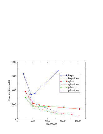
Figure 1: Performance of the original code with varying process counts and layouts

To investigate this performance difference further we performed some in depth profiling on xyles at 2048 processes and yxles on 1536 processes. For this profiling we collected some data (averaged across the processes running the simulation) on the MPI communications performed, which is presented in Table II. The data on MPI message sizes is summarised by reporting statistics on groups of message sizes.

TABLE II: Profiling results of GS2 using the xyles and yxles layouts

Layout	Process Count	Data Transform	Profile Metric	Profile Result
xyles	2048	g_lo $\rightarrow$ xxf_lo	MPI Msg Bytes	1499904000.0
			MPI Msg Count	12000.0 msgs
			64KB $\leq$ MsgSz $<$ 1MB Count	12000.0
		xxf_lo $\rightarrow$ yxf_lo	MPI Msg Bytes	49152000.0
			MPI Msg Count	4000.0 msgs
			4KB $\leq$ MsgSz $<$ 64KB Count	4000.0
		yxf_lo $\rightarrow$ xxf_lo	MPI Msg Bytes	374976000.0
			MPI Msg Count	3000.0 msgs
			64KB $\leq$ MsgSz $<$ 1MB Count	3000.0
		xxf_lo $\rightarrow$ g_lo	MPI Msg Bytes	12288000.0
			MPI Msg Count	3000.0 msgs
			4KB¡= MsgSz $<$ 64KB Count	1000.0
yxles	1536	g_lo $\rightarrow$ xxf_lo	MPI Msg Bytes	2006592000.0
			MPI Msg Count	12450.5 msgs
			256B $\leq$ MsgSz $<$ 4KB Count	125.0
			4KB $\leq$ MsgSz $<$ 64KB Count	1895.8
			64KB $\leq$ MsgSz $<$ 1MB Count	10429.7
		xxf_lo $\rightarrow$ yxf_lo	MPI Msg Bytes	2749824000.0
			MPI Msg Count	5487.0 msgs
			256B $\leq$ MsgSz $<$ 4KB Count	26.0
			4KB $\leq$ MsgSz $<$ 64KB Count	380.2
			64KB $\leq$ MsgSz $<$ 1MB Count	5080.7
		yxf_lo $\rightarrow$ xxf_lo	MPI Msg Bytes	687456000.0
			MPI Msg Count	1371.7 msgs
			256B $\leq$ MsgSz $<$ 4KB Count	6.5
			4KB $\leq$ MsgSz $<$ 64KB Count	95.1
			64KB $\leq$ MsgSz $<$ 1MB Count	1270.2
		xxf_lo $\rightarrow$ g_lo	MPI Msg Bytes	501648000.0
			MPI Msg Count	3112.6 msgs
			256B $\leq$ MsgSz $<$ 4KB Count	31.2
			4KB $\leq$ MsgSz $<$ 64KB Count	474.0
			64KB $\leq$ MsgSz $<$ 1MB Count	2607.4

From the results shown in Table II we can see that for the transform between g_lo and xxf_lo (and the inverse) both xyles and yxles show similar characteristics, using roughly 12000 messages for the first transform. However, given that yxles is using $75\%$ of the processes that xyles it is surprising that it is actually sending $25\%$ more data.

When we look at the communications required for transforming from xxf_lo to yxf_lo, however, we can see there is a very large difference in the amount of data sent between the two layouts. Using yxles generates approximately 55 times more data traffic than xyles with only $25\%$ more messages. The large difference in the amount of data that is sent using a similar number of messages, is explained by the fact that much larger messages are communicated in the yxles case than in the xyles case.

III-C Discussion of the performance impact of data distributions

Data structures with two indices are used during the 2-D FFT transformation chain from k-space into position space. The first index is the index along which the FFT is to be performed, and the second index is of the xxf or yxf-type, suitable for 1D FFTs in the X or Y directions respectively.

Here we focus on the distribution of a data structure using an xxf-type index. (The discussion for a yxf-type structure is essentially the same, except that the first index corresponds to Y). As previously discussed, the 2nd xxf-type index is a compound of the indices Y,ig,isgn,l,e,s. For all layouts described by a GS2 layout string that ends l,e,s, the compounded indices will be ordered as above. In a parallel GS2 calculation, the array volume associated with this last index gets distributed by calculating a blocksize as outlined in Equation 6. If the integer divide on the right hand side leaves any remainder, the formula rounds up the blocksize to the nearest integer to ensure that all the data is allocated.

The ingen tool typically guides the user to select a process count that divides the g_lo cleanly across cores. With layout xyles or yxles, ingen will recommend core counts where the indices les are well distributed for g_lo. Any recommended core count that exceeds the product les, will be an integer multiple ${\tt j}*{\tt les}$, and will have l,e,s maximally distributed. At such core counts, the xxf_lo layout, with compound index ordered Y,ig,isgn,l,e,s, will also have l,e,s maximally distributed. Therefore, the remaining elements of the xxf_lo compound index, Y,ig,isgn, must be distributed over j processes. While isgn has a range of 2, the allowed range for ig is always has an odd number which commonly does not factorise well (or may even be prime). We will see shortly that this can lead to blocksizes for xxf_lo and yxf_lo from Equations (6) and (4), that have unfortunate consequences for communication.

Figure 2 shows the situation where the three indices Y,ig,isgn can be evenly divided across four processes, which is only possible if Y is even. As Y is the fastest index, the split between the data going to the lower or the higher task rank will occur in the middle of a Y-column.

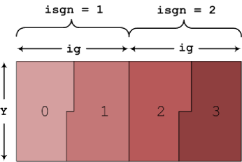
Figure 2: Example of how the array projection spanned by Y, ig, isgn will be distributed between 4 processes, when the allowed range for Y is divisible by two.The colour indicates the process-id to which each piece of data is assigned.

If in our example, the allowed range for Y were odd the work would not divide evenly over 4 processes, as shown in 3 where the sub-array spanned by Y, ig, isgn is not exactly divisible by the number of processes and this results in most processes being allocated the same amount of data, but can very easily result in the situation, especially for large problems and process counts, where one or more of the last processes in the simulation will have little or no work assigned to them (i.e. their blocksize will be small or zero). While for large task counts this will not result in a significant load imbalance in the computational work, it can dramatically increase the level of communication that is required in the redistribution routines between xxf_lo and yxf_lo.

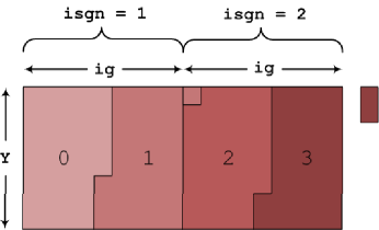
Figure 3: Example of a decomposition that does not evenly split. In this example process 0 gets more than ½ of the first Y-ig box, and process 1 is then assigned some data points from the second box. When all the data from the first two boxes are assigned, process 3 will still require data from the next pair of Y-ig boxes, as indicated by the small box to the right of the main picture.

We now consider the amount of data that must be passed between different processes during the transpose transformation between xxf_lo and yxf_lo. Figure 4 illustrates what happens when both indices split evenly across the processes, clarifying that only a small amount of the data held by a process needs to be transferred between neighbouring processes. Figure 3 showed that, if xxf_lo or yxf_lo data spaces do not divide evenly across all processes, the equal blocksizes allocated to each process a will ensure all the data is allocated, but not that all processes will be allocated data. Figure 3 demonstrates that this leads to an overspill, where some processes are allocated data from more than one l, e, or s index. Furthermore, not all processes will be allocated with the full blocksize: there will be at least one task with a smaller allocation of data, and there may be further tasks which are allocated with no data. The number of idle processes can be calculated as shown in Equation 8 (where $xxf\_totalsize$ is defined in Equation 5 and $xxf\_blocksize$ is defined in Equation 6).

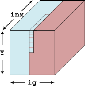
Figure 4: Example of the data to be transferred between cores when transposing from xxf_lo to yxf_lo. For xxf_lo, the lower ranking process holds the blue data and the shaded region. The higher ranked process holds the red data. During the transformation the shaded region needs to be transferred from the lower to the higher rank. There is a similar region in the bottom rear of the cube, not visible in the figure, which needs transferring from the higher ranking to the lower ranking process.

$$xxf\_usedprocs=\frac{xxf\_totalsize}{xxf\_blocksize}$$ (7)

$$xxf\_idleprocs=number\>of\>processes-xxf\_usedprocs$$ (8)

Similarly the idle processes when using yxf_lo can be determined as follows:

$$yxf\_usedprocs=\frac{yxf\_totalsize}{yxf\_blocksize}$$ (9)

$$yxf\_idleprocs=number\>of\>processes-yxf\_usedprocs$$ (10)

If the numbers yxf_idleprocs and xxf_idleprocs differ significantly, it can easily be shown that large MPI messages will be required in the transforms between xxf_lo and yxf_lo. Indeed this can easily arise, as the spatial dimensions in the compound xxf_lo and yxf_lo indices, Y and inx respectively, are different. Y and inx may have quite different prime factors, and one layout may split evenly with no idle processes while the other does not.

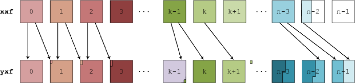
Figure 5: Example of the data redistributions required when xxf_lo and yxf_lo have different numbers of idle processors. The colours label the data regions that are stored by each processor in xxf_lo.

Figure 5 demonstrates clearly how the amount of data to be sent to a different process increases linearly with increasing task number. If the difference between yxf_idleprocs and xxf_idleprocs is larger than 1, the highest ranking processes (those of rank $k$ and above in Figure 5) will have to transfer all of their data to different processes. Where the difference is less than one, all processes will keep some of their data.

III-D Analysis of communication costs

We now estimate the amount of data that must be communicated via MPI for these two cases. It is helpful to define variables

$$delta\_idle\_proc=dabs(yxf\_idleprocs-xxf\_idleprocs)$$ (11)

$$total\_redist\_data=inx*xxf\_totalsize$$ (12)

The total amount of data to be transferred during the redistribution (e.g. inserted into the communication network) can be estimated as shown in Listing 1.

⬇

1if ( delta_idle_proc .le. 1 ) then

2 total_trans_data = 0.5D0 * delta_idle_proc * total_redist_data

3else

4 total_trans_data = (1.0d0 $-$ 1.0d0/(2.0d0 * delta_idle_proc)) * total_redist_data

5endif

Listing 1: Total amount of data to be be transferred

These estimates should be correct for large task counts, which is the situation of interest in this paper. As the difference between the numbers of idle processors approaches 1, a significant portion of the data held during the transformation needs to be communicated between processes across the network. This has to be contrasted with the case where the data splits evenly across processors. In that case, a much smaller portion of the total data has to be passed via MPI, typically only a few percent of the total data space.

IV Unbalanced Decomposition

The functionality that transforms data from g_lo to xxf_lo involves moving from a data distribution when ig and isgn are local on each process (i.e. each process has the full dimensions of ig and isgn for a given combination of x,y,l,e,s) to one where X is local (i.e. each process has the full dimension of inx for a given combination of Y,ig,isgn,l,e,s). The transformation to yxf_lo is to a data distribution where iny (where iny full size of Y without any points dropped to facilitate the de-aliasing filter) is guaranteed to be local (for any given combination of inx,ig,isgn,l,e,s).

When running GS2 on large process counts ($>$ l * e * s processes) these transformations will require unavoidable data communications, particularly the transform from g_lo to xxf_lo (which moves from ig,isgn local to inx local) as at high core counts the xxf_lo data distribution will have to split up isgn and possibly ig (depending on the process count) which are local dimensions in g_lo.

However, the complexity of the redistribution and the quantity of data to be communicated will depend on how split up the data is. If the data dimensions to be redistributed are only split across pairs of processes in a balanced fashion then the required message sizes and number of messages will be lower than if the data must be split up across a larger number of different processes.

Furthermore, if the decomposition is undertaken optimally it should be possible to ensure that the redistribution between g_lo and xxf_lo keeps both inx and Y as local as possible, thereby reducing or eliminating completely the MPI communication cost of the xxf_lo to yxf_lo step.

Therefore, we have created unbalanced decomposition functionality to optimise the data distribution in the xxf_lo and yxf_lo data layouts. This replaces the current code to calculate the block of xxf_lo and yxf_lo data that each process owns, moving from a uniform blocksize to adopting two different blocksizes for the process counts when the data spaces do not exactly divide by the number of processes used.

The new, unbalanced decomposition, uses the process count to calculates which indices can be completely split across the processes. This is done by iterating through the indices in the order of the layout (so for the xxf_lo data distribution and the xyles layout this order would be s,e,l,isgn,ig,Y) dividing the number of processes by each index until a value of less than one is reached. At this point the remaining number of processes is used, along with the index to be divided, to configure an optimally unbalanced decomposition, by deciding on how to split the remaining indices across the remaining cores that are available. If this index dimension is less than the number of cores available, then the index dimension is multiplied by the following index dimension until a satisfactory decomposition becomes possible.

Figure 6 demonstrates the decomposition of the example in Figure 3 when computed using the new unbalanced decomposition functionality.

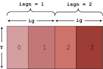
Figure 6: Example of an decomposition that does not evenly split but has been decomposed using the unbalanced decomposition functionality.

The drawback of using an unbalanced decomposition approach is that this makes a controlled sacrifice by introducing computational load imbalance (i.e. some processes are allocated more computational work than others) which is generally to be avoided for parallel programs. The assumption that we are making is that the modest computational load imbalance introduced is much less significant than the drastic reduction in communications that can be achieved. However, this assumption will only hold true if the amount of computational imbalance is not too large. A computational imbalance of $100\%$ (so some processes acquire twice as much computational work as others for the non-linear calculations) is likely to negate the communication performance improvement from the unbalanced decomposition. Therefore, with the new decomposition functionality we allow users to specify a maximum threshold to the amount of computational imbalance allowed. If this threshold would be exceeded by using the unbalanced decomposition algorithm, then the original decomposition functionality with uniform blocksizes is utilised.

V Unbalanced Performance

We assessed the impact of the new unbalanced decomposition functionality on the performance of two of the simulations that appeared in Table I: the xyles layout running on 2048 processes; and the yxles layout running on 1536 processes. The run times of the original code and of the new unbalanced code are compared in Table III, and in Figure 7. For the yxles layout the imbalance created by the new code (the difference in size between the small and large blocks) is approximately $5\%$ and for xyles it is approximately $7\%$.

TABLE III: Comparison of the original and unbalanced GS2 runtimes

Layout	Process Count	Version	Runtime (seconds)
xyles	2048	Original	138
		Unbalanced	138
yxles	1536	Original	165
		Unbalanced	141

The 1536 process simulations yxles simulations demonstrate that the unbalanced code significantly reduces the overall runtime of the original code, with the unbalanced optimisation saving around $15\%$ of the GS2 runtime. This is in spite of our introduction of a computational load imbalance of around $5\%$ for the non-linear calculations. Thus it is clear that the unbalanced decomposition can significantly improve GS2’s performance.

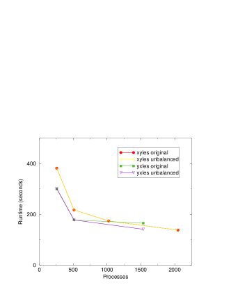
Figure 7: Performance comparison of the unbalanced code with the original results collected.

However, if we look at the 2048 process xyles results the unbalanced optimisation makes little difference to the overall runtime. Further in depth profiling of the code reveals that the unbalanced decomposition does significantly reduce the runtime associated with the MPI communications, but this communications overhead is much less significant for this simulation layout and process count. The MPI communications for the yxles layout on 1536 processes takes around 6 times as long as for the xyles layout on 2048 processes. The unbalanced optimisation still does exactly what we would expect in the xyles simulation on 2048 processes: it significantly reduces the cost of the communications, but it does not significantly reduce the overall runtime as this simulation requires much less MPI communication.

Performance profiling reveals that the unbalanced functionality reduces the requirement of MPI communications in the xxf_lo to yxf_lo transformation in both test cases. Table II shows that the MPI communications required for the xyles run were anyhow very small (small numbers of small messages), but that MPI messages were much more significant in both size and number for the yxles run.

This performance difference is not solely predicated on the layout used, but also on the number of processes used. In the benchmark simulation using xyles layout on 2048 processes, the xxf_lo total size exactly divides by the number of processes, allocating every process with a blocksize of 496. In a simulation with the same layout using only 1536 processes, the same data space cannot be divided across all processes with an equal blocksize. The exact blocksize would be $661\frac{1}{3}$ in this case, so the original code rounds this up to the nearest integer and sets a uniform blocksize of 662. This results in the final process being allocated with no xxf_lo data and the second last process being allocated with only half a block, thus generating a large communication overhead to transform the data, as illustrated in Figure 5.

VI Conclusions

We have investigated the performance of the GS2 simulation code and discovered that the choices made to incorporate both linear and non-linear calculation (in k-space and position space respectively) in a single code can introduce performance issues for a parallel code. In particular, a process count that is optimal for the linear computation may not be optimal for the non-linear computation (which requires redistribution of the large data arrays), and the optimal linear process count may adversely affect the performance of the non-linear computation. Conversely, choosing a process count that is optimal for the non-linear computations, could adversely impact on the performance of the linear computations

Transformations between different layouts are required in order to carry out different parts of the GS2 calculation. It is desirable for the data in each layout to be divided evenly across all processes, so that in each part of the calculation, every process has an equal blocksize of data to work with. A process count can always be chosen so that this is achieved for one of the required layouts, but an equal distribution of data in the other layouts cannot be guaranteed. If equal blocksizes are allocated, it is possible that for some layouts there will be a number of processes that are allocated with no data. Even when there are only a small number of empty processes, our performance analysis has revealed that the increased MPI communication overhead has adverse performance implications that can be very significant.

From the computational point of view there should be negligible impact on the performance of a 1536 core simulation if 1½ processes are empty, as this corresponds to only $0.1$% of the total processes. However, we have demonstrated that for the transforms required in GS2, this small difference in the number of cores required to store the data in each layout, can lead to a huge difference in the amount of data requiring to be communicated: this can increase from a few percent to a very significant fraction of the total data set.

Making a small change to the decomposition algorithm, to use two different blocksizes instead of uniform blocksizes, enables the data space to be split more evenly across all of the processes. This change can drastically reduce the communications that are required for transformations between layouts.

Whilst this paper has focussed on the GS2 simulation code, the main techniques and algorithms that GS2 exploits are very widely used in scientific computing: e.g. the different data layouts that are required for the separated linear and non-linear parts of the calculation, and the exploitation of FFT algorithms. The functionality we have outlined here should be widely applicable in many other scientific codes.

References

- [1] M. Kotschenreuther, “Comparison of initial value and eigenvalue codes for kinetic toroidal plasma instabilities,” Computer Physics Communications, vol. 88, no. 2-3, pp. 128–140, 1995. [Online]. Available: http://linkinghub.elsevier.com/retrieve/pii/001046559500035E
- [2] W. Dorland, F. Jenko, M. Kotschenreuther, and B. N. Rogers, “Electron temperature gradient turbulence.” Physical Review Letters, vol. 85, no. 26 Pt 1, pp. 5579–5582, 2000. [Online]. Available: http://link.aip.org/link/PHPAEN/v7/i5/p1904/s&Agg=doi
- [3] “Hector.” [Online]. Available: http://www.hector.ac.uk