The Light Element Abundance Distribution in NGC 5128 from Planetary Nebulae

Abstract

Context. Planetary nebulae in the nearest large elliptical galaxy provide light element abundances difficult or impossible to measure by other means in a stellar system very different from the galaxies in the Local Group.

Aims. The light element abundance pattern from many planetary nebulae (PNe) at a range of radial distances was measured from optical spectroscopy in the elliptical galaxy NGC 5128, which hosts the radio source Centaurus A. The PN abundances, in particular for oxygen, and the PN progenitor properties are related to the galaxy stellar properties.

Methods. PNe in NGC 5128 covering the upper 4 mag. of the luminosity function were selected from a catalogue. VLT FORS1 multi-slit spectra in blue and red ranges were obtained over three fields at 3, 9 and 15^′ projected radii (4, 8 and 17 kpc, for an adopted distance of 3.8 Mpc) and spectra were extracted for 51 PNe.

Accurate electron temperature and density diagnostics are usually required for abundance determination, but were not available for most of the PNe. Cloudy photoionization models were run to match the spectra by a spherical, constant density nebula ionized by a black body central star. He, N, O and Ne abundances with respect to H were determined and, for brighter PN, S and Ar; central star luminosities and temperatures are also derived.

Results. Emission line ratios for the 51 PNe are entirely typical of PN such as in the Milky Way. The temperature sensitive [O III]4363Å line was weakly detected in 10 PNe, both [O II] and [O III] lines were detected in 30 PNe, and only the bright [O III]5007Å line was detected in 7 PN. For 40 PNe with Cloudy models, from the upper 2 mag. of the [O III] luminosity function, the most reliably estimated element, oxygen, has a mean 12+Log(O/H) of 8.52 with a narrow distribution. No obvious radial gradient is apparent in O/H over a range 2-20 kpc. Comparison of the PN abundances with the stellar population, from the spectra of the integrated stellar light on the multi-slits and existing photometric studies, suggests an average metallicity of [Fe/H]=-0.4 and [O/Fe]=0.25.

Conclusions. The masses of the PN central stars in NGC 5128 deduced from model tracks imply an epoch of formation even more recent than found for the minority young population from colour magnitude studies. The PN may belong to the young tail of a recent, minor, star formation episode or derive from other evolutionary channels, perhaps involving binary stars.

1 Introduction

Planetary nebulae provide a multi-facetted probe of the galactic environment. As a short-lived product of the evolution of low mass stars, they sample the bulk, by both number and mass, of the stellar population of galaxies of all Hubble types. Their size makes them unresolved from the ground at distances greater than $\sim$1 Mpc but their strong emission lines makes them easy targets for observational work, even when observed against the high stellar background of a galaxy bulge. These advantages have been exploited in a number of distinct areas. Statistics of PN in galaxies of various types show a late time indicator of the star formation rate through the luminosity specific PN frequency $\phi$ ( Ciardullo et al. Ciardullo89 (1989)). The PN luminosity function (PNLF), despite theoretical difficulties, still proves to be a powerful distance method (Jacoby et al. Jacoby92 (1992); Ciardullo et al Ciardullo02 (2002)). The radial velocity, simply measured from one emission line, provides a kinematic test particle for study of the galaxy potential and in intra-cluster gas of the cluster potential and turbulence (Arnaboldi et al. Arnaboldi (2003)). The abundances of a number of light elements can be measured from emission line ratios in PN spectra, such as He and N and, in particular, the $\alpha$-elements O, Ne, S and Ar, which are difficult to study in all but high resolution and high signal-to-noise spectra of individual stars.

As the closest example of a large early-type galaxy, NGC 5128 (Hubble type S0p) occupies a central place in studies of resolved stellar populations in a galaxy different to the Milky Way and M31. This large elliptical galaxy in the Centaurus group shows signs of major activity with an active nucleus, Faranoff-Riley Class I radio lobes, presence of dust and young stars in its inner region (Graham Graham (1979)), a young ($\sim$0.3 Gyr) tidal stream (Peng et al. Peng02 (2002)) and stellar shells in its outer regions (Malin et al. Malin (1983)); see Israel (Israel (1998)) for an earlier review. This activity can be attributed to a minor merger which has had little influence on the bulk of the older passively evolving population (Woodley Woodley06 (2006)), making NGC 5128 a nearby exemplar of more distant massive early-type galaxies; Harris (Harris10 (2010)) provides a recent review of the underlying galaxy properties. The spectroscopy of globular clusters by Beasley et al. (Beasley (2008)) indicates typical ages of 7-8 Gyr from stellar population fitting, reinforcing the presence of a large-scale intermediate age star formation episode. Fits to deep colour-magnitude diagrams also provide evidence for a minority, much younger, population of age 2-4 Gyr (Rejkuba et al. Rejkuba11 (2011)).

As representative of the low mass stars, planetary nebulae in NGC 5128 have been catalogued over a period of two decades, beginning with the catalogue of Hui et al. (1993a ). 785 PN were discovered by [O III]5007Å emission line and off-band imaging; from the PN [O III] magnitudes Hui et al. (1993b ) determined a PNLF distance of 3.5 Mpc. Independent measurements from the Mira period-luminosity relation and the luminosity of the tip of the red giant branch (Rejkuba et al. Rejkuba05 (2005)), surface brightness fluctuations (Tonry et al. Tonry (2001)), globular cluster luminosity function (Harris et al. Harris88 (1988)) and 42 classical Cepheid variables (Ferrarese et al. Ferrarese (2007)) result in distance estimate in the range 3.4 to 4.1 Mpc. Harris et al. (HRH10 (2010)) present a comprehensive review of distance estimates to NGC 5128, and recommend a best-estimate of 3.8 Mpc, which is adopted here (distance modulus 27.90mag.). Peng et al. (Peng04 (2004)) extended the original catalogue of PN and found a further 356 PN by filter imaging; 780 out of a total of 1141 were spectroscopically confirmed. Further emission line mapping and follow-up intermediate dispersion spectroscopy has extended this list to over 1200 confirmed PN (Rejkuba & Walsh RejWal (2006)). This number of PN makes NGC 5128 a rich source for statistical extra-galactic PN studies, rivalled only by the Milky Way and M 31 (Merrett et al. Merrett06 (2006)).

Since there are both a large number of PN and they have been catalogued to large galactocentric distances (to 80 kpc along the major axis by Peng et al. (Peng04 (2004))), the radial velocities allow the dynamics of the halo mass distribution to be studied. Hui et al. (Hui95 (1995)) measured [O III] radial velocities for 431 out of their 785 catalogued PN. The offset of the rotation axis from the minor axis was attributed to evidence of triaxiality; fitting the rotation curve and velocity dispersion revealed a radially increasing mass-to-light ratio and hence the presence of a dark matter halo. Peng et al. (Peng04 (2004)) extended the PN kinematic work to 780 PN and showed the large rotation along the major axis but with a pronounced zero-velocity twist produced by the triaxial-prolate mass distribution. The kinematics of the large population of globular clusters (with 563 available radial velocities – Woodley et al. Woodley10 (2010), Woodley et al. Woodley07 (2007), Beasley et al. Beasley (2008)) show similar kinematics to the PN but with small differences, such as lower rotation amplitude (Woodley et al. Woodley07 (2007)).

The NGC 5128 globular clusters (GCs) also provide fundamental evidence of the star formation history. Of the 605 confirmed GCs in NGC 5128 (Woodley et al. Woodley07 (2007), Woodley et al. Woodley10 (2010)), more than half have metallicity measurements and they divide roughly half and half into metal rich and metal poor above and below [Fe/H]$=-1.0$. The metal poor GCs ([Z/H]$\sim-1.3$) are older with ages similar to Milky Way GCs and the metal rich GCs (Peng et al. Peng04 (2004); Beasley et al. Beasley (2008)) have intermediate ages (4-8 Gyr) and metallicity ([Z/H]$\sim-0.5$). There are many more GC candidates (e.g. Harris et al. Harris04 (2004)) and the total number of GCs has been estimated at around 1300 (Harris Harris10 (2010)).

NGC 5128 is close enough that individual stars can be resolved with HST imaging (and from the ground with adaptive optics in the near-IR) and several studies have been obtained outside of the bright bulge where crowding is lower. Soria et al. (Soria (1996)) detected the Red Giant Branch (RGB) and the Asymptotic Giant Branch (AGB) from intermediate age stars. The same field was followed up with NICMOS photometry and the IR colour magnitude diagram shows stars well above the tip of the red giant branch for old stars, confirming the presence of intermediate age stars (Marleau et al. Marleau (2000)). Colour magnitude diagrams from HST WFPC2 were constructed for two halo fields at projected radii of 19 and 29 kpc (Harris et al. Harris99 (1999); Harris et al. Harris00 (2000)). The colour magnitude diagrams are dominated by old stars. Under the assumption that the ages of the stars in NGC 5128 are similar to those of old globular clusters in our Galaxy, the mean metallicity of the two fields was found to be similar at [Fe/H]$\sim-0.4$ with about one third of the stars in a metal poor component and the rest metal rich. The metallicities in the halo fields were compared by Harris et al. (Harris02 (2002)) to the metallity distribution function (MDF) in a field at 7.4kpc, containing a mixture of outer bulge and inner halo. A broad MDF was found as in the halo fields, peaking at [Fe/H]$\sim-0.4$; but subtracting the MDF of the halo fields reveals a peak at slightly higher metallicity ($\sim-0.2$). Much deeper ACS imaging by Rejkuba et al. (Rejkuba05 (2005)) in a halo field at 36 kpc reached to the horizontal branch (core helium burning population) as well as showing the red giant branch, red clump and AGB bump. Again a broad MDF was found with an average metallicity of $-0.64$, but with a broad tail to higher metallicity ($>0$). The age sensitive indicators imply an average age for the halo of 8${}^{+3}_{-4}$ Gyr. Comparison of the MDF in the four fields shows the peak shifting to lower metallicity with increasing projected radius but the distribution is similarly wide at all radii.

In order to determine light element abundances of PN in NGC 5128 fairly high signal-to-noise spectroscopy is required. Close to the inner bulge the stellar continuum surface brightness is too high and only the strongest few lines can be measured. However in the outer regions by selecting bright PN, diagnostic lines of He, Ne, Ar and S as well as the brighter lines of O and N can be measured and abundances derived. Walsh et al. (Walsh99 (1999)) performed deep ESO 3.6m long slit spectra of a few selected PN with a long slit spectrograph and measured lines in addition to the brightest line ([O III]5007Å) in five PN. O/H could be determined in two PN and values of 12 + Log(O/H) $\sim$8.5 (i.e. [O/H] - 0.2, adopting the Solar oxygen abundance of 8.69 from Scott et al. (Scott (2009))) were derived. This initial work has been expanded to deeper spectra of many more PNe with the ESO VLT and FORS1 instrument in multi-slit mode. In section 2 the observations are described and the reduction of the spectra and derivation of the abundances are presented in section 3. The results for the PN line fluxes and derived abundances both for the individual PN and for summations of many spectra are presented in section 4. Since the diagnostic lines for electron temperature and density, important for abundance determination, are weak or undetected, photoionization modelling of all well-detected lines was undertaken using Cloudy and is described in section 5. Consideration of the lack of a gradient in the PN O abundances, comparison of the results with the stellar, photometrically-derived metallicity, and relation of the PN to the stellar populations in NGC 5128 are discussed in section 6. Conclusions are collected in section 7.

2 Observations

2.1 FORS imaging and spectroscopy

The European Southern Observatory Very Large Telescope (VLT) FORS1 instrument mounted on VLT Unit Telescope 1 was used for the observations described. FORS1 has a number of modes for imaging; for spectroscopy, long slit, multi-slit, or multi-slit mask are available (see Appenzeller et al. Appenzeller (1998) for details). The multi-object mode (MOS) allows 19 slitlets of height varying from 20 to 22 $\arcsec$ to be placed over a 6.8$\times$6.8$\arcmin$ field of view. In the regions of NGC 5128 where PNe were catalogued by Hui et al (1993a ) and (1993b ), the surface density is such that there are usually enough PNe to be able to fill the slitlets, thus ensuring an optimal match between target density and instrument multiplex. This match was realised in practice for regions over the bright disk of NGC 5128, whilst in the outer regions, around 50% of the slitlets could be utilised. Three regions were selected for MOS spectroscopy to fulfill the following criteria: sample the inner and outer regions at a range of effective radii to detect any abundance gradient from the PNe; sample the major and minor axes; ensure that some of the brightest PNe were observed to maximize the probability of detecting the faintest line species; collect as many PN spectra as possible. Not all of these criteria are mutually consistent, but the three regions selected at radial offset distances of 3.4, 8.7 and 15.4$\arcmin$ provided spectra of 51 PNe at a range of m_5007A ( m_5007A = -2.5 log F_λ (erg cm^-2 s^-1) -13.74; Jacoby Jacoby89 (1989)) from 23.5 to $>$27.0 mag.

2.1.1 Pre-imaging

Direct images with FORS1 and a narrow band [O III] filter (called OIII+50, centred at 5005Å and FWHM 57Å) were obtained in December 1999-January 2000 in service mode. Tab. 1 lists details of the imaging observations whose primary purpose was to provide images for the MOS slit assignment using the FIMS tool. The standard resolution collimator was used giving a field of 6.8$\times$6.8$\arcmin$ with a pixel size of 0.2$\arcsec$ per pixel. The field names are taken from those of Hui et al. (1993a ). A companion filter (actually a redshifted [O III] filter OIII/6000, centred at 5109 Åwith FWHM 61Å) was also used to obtain an [O III] off-band subtraction to confirm the reality of the PNe; all the previously catalogued PNe in the fields were confirmed as [O III] emission line objects. Seeing at the time of observations was between 0.5 and 1.2$\arcsec$.

Table 1: FORS1 pre-imaging observations

Position	$\alpha$              $\delta$	[O III] Exp	Cont.	Date
(radius, kpc)	h   m   s       ∘    $\arcmin$    $\arcsec$	(sec)	(sec)
F56 (9.6)	13 25 50.6 -43 06 09.2	2$\times$480	2$\times$220	1999 12 27
F42 (3.8)	13 25 09.0 -43 02 29.3	2$\times$480	2$\times$220	2000 01 13
F34 (17.0)	13 24 47.2 -43 13 32.2	2$\times$480	2$\times$220	2000 01 13

2.1.2 MOS Spectroscopy

FORS1 MOS observations in service mode were conducted in three sessions. Tab. 2 lists the salient details in chronological order. To cover the wavelength range with useful diagnostic emission lines (essentially from [O II]3726,3729Å to beyond [O II]7320,7330Å), two grisms were employed: grism 600B (called GRIS_600B+12) has a dispersion of 1.2Å/pixel and, for a centred MOS slitlet, a wavelength coverage of 3450 to 5900Å; grism 300V (named GRIS_300V+10 and used with a GG435 blocking filter) has a lower dispersion of 2.7Å/pix and a coverage of 4450 to 8650Å. The overlap region between both spectra is 4500-5900Å  thus allowing at least the strong [O III]4959,5007Å lines to be used to tie the two spectra to a common flux scale. The slit width for the campaigns in 2000 and 2001 was 0.8$\arcsec$ whilst the observations in 2003 had a slit width of 1.0$\arcsec$. The resulting spectral resolutions are 4.8 and 6.0Å for 600B and 10.7 and 13.4Å for 300V observations respectively. The supporting observations of the spectrophotometric standard stars for flux calibration, which were taken with a broad slit of 5^′′ width, are listed in Tab. 3.

Table 2: FORS1 PN spectroscopic observations

Position	$\alpha$       $\delta$	Grism	Exp.	Date	Seeing
	h   m   s       ∘    $\arcmin$    $\arcsec$		(sec)		($\arcsec$)
F56	13 25 50.6 -43 06 09.2	600B	4$\times$2400	2000 05 02	0.8-1.2
F56	13 25 50.6 -43 06 09.2	300V	2$\times$2400	2000 05 02	0.8-1.2
F42	13 25 09.0 -43 02 29.3	600B	2$\times$1500	2001 03 22	0.8
F34	13 24 47.2 -43 13 32.2	600B	2$\times$1500	2001 03 24	0.9
F34	13 24 47.2 -43 13 32.2	600B	2$\times$1500	2001 03 27	0.8
F42	13 25 09.0 -43 02 29.3	600B	2$\times$1500	2001 03 27	0.7
F34	13 24 47.2 -43 13 32.2	300V	2$\times$1320	2003 03 25	0.7
F34	13 24 47.2 -43 13 32.2	600B	8$\times$1320	2003 04 08	0.5
F42	13 25 09.0 -43 02 29.3	300V	2$\times$1320	2003 04 24	1.0
F42	13 25 09.0 -43 02 29.3	600B	3$\times$1320	2003 04 24	1.0
F42	13 25 09.0 -43 02 29.3	600B	3$\times$1320	2003 04 30	0.6
F42	13 25 09.0 -43 02 29.3	300V	2$\times$1320	2003 04 30	0.5
F56	13 25 50.6 -43 06 09.2	300V	2$\times$1320	2003 05 05	0.5
F56	13 25 50.6 -43 06 09.2	600B	4$\times$1320	2003 05 05	0.6
F34	13 24 47.2 -43 13 32.2	300V	2$\times$1320	2003 06 02	1.1
F56	13 25 50.6 -43 06 09.2	600B	2$\times$1320	2003 07 21	1.0
F56	13 25 50.6 -43 06 09.2	300V	2$\times$1340	2003 07 22	0.4

Table 3: FORS1 spectrophotometric standard star observations

Star	Grism	Exp.	Date
		(sec)
LTT 7379	600B	25	2000 05 02
LTT 7379	300V	7	2000 05 02
LTT 7379	600B	25	2001 03 24
LTT 7379	600B	25	2001 03 27
EG 274	600B	30	2003 04 08
LTT 7379	600B	25	2003 04 24
LTT 7379	300V	7	2003 04 24
LTT 7379	600B	25	2003 04 30
LTT 7987	600B	100	2003 05 05
LTT 7987	300V	30	2003 05 05
LTT 7987	300V	30	2003 06 02
LTT 7379	300V	7	2003 07 22

3 Reduction and analysis

All the data frames (flats, science frames on PN and standard stars) were bias subtracted using master bias frames provided by the ESO reduction pipeline contemporaneous with the observing data. Standard IRAF routines were used for the reduction. Pixel-to-pixel flat fields were constructed from dome flats by extracting the 2D area of each slitlet, collapsing in the cross-dispersion direction, box car smoothing in the dispersion direction and dividing the dome flat by the smoothed version. Identical reductions were performed for the bluer (600B grism) and redder (300V grism) spectra. Wavelength calibration was achieved by fitting 4th order Chebyshev polynomials to the dependence of pixel position on wavelength for the arc lamp lines on each slitlet separately. The separate slitlet images, rebinned to an identical wavelength scale, were then recombined into a single image which was corrected for atmospheric extinction. Individual exposures were combined with clipping to remove discrepant pixels caused by detector bad pixels and cosmic ray events. Flux calibration was achieved by observations of one or more spectrophotometric standard stars, the ones applied being listed in Tab. 3. The standard star spectra were analysed in an identical way to the PN, except that the one slitlet pertaining to the standard star was reduced. In the few cases where a standard star was not available in the same configuration as the PN on the night of observation, a standard star from another night had to be used. In general conditions were good or photometric, and no large flux calibration discrepancies were found between spectra of the same field observed in different runs (see Tab. 2). Narrow band magnitudes for the spectrophotometric standards were taken from Hamuy et al. (Hamuy (1994)) and the PN spectra were flux calibrated using iraf.noao.onedspec routines. Fig. 1 shows an example of the reduced multi-slit spectra for field F56. The unequal wavelength coverage of the spectra is dependent on the relative position of the target centred slitlet within the field. Thus a target to the right edge of the field is truncated to the red but extends to lower wavelengths than a target in the centre of the FORS1 MOS field.

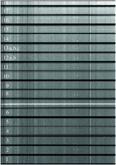
Figure 1: The reduced MOS spectra for field F56 taken with grism 600B (data from May 2000). Eighteen of the 19 slitlets are shown for a wavelength range from about 3970 to 5520Å and the numbering of the extracted PN spectra are indicated. Two slitlets show multiple PN spectra. The higher background stellar continuum towards the top of the image corresponds to lower galactocentric distance.

Fig. 1 demonstrates that there can be more than one PN per slitlet; in some cases this was planned, by placing the slitlet such that two PN from the Hui et al. catalogue lay on the slit, but in some cases in the two inner fields, PN were spectroscopically detected that were not present in the Hui et al. catalogue, on account of their faintness or proximity to another catalogued PN. These previously uncatalogued PN typically had m${}_{5007A}>27$mag. On the basis of the strongest line - [O III]5007Å - the number of PN detectable in the three fields were: 21 in F56; 21 in F42; and 9 in F34. On each slitlet, regions distinct from the PN spectra were located and used to subtract the background, with a 1st or 2nd order fit in the cross-dispersion direction. In determining the spectra of the PN, no attempt was made to perform a separate sky background subtraction since there is galaxy background at all slitlet positions, except perhaps for the slitlets at largest galactocentric distance in the outermost field (F34). 1D spectra of each PN were formed by summing the background subtracted signal along the slit; 7-9 pixels (1.4-1.8$\arcsec$) were used to collect around 60 to 70% of the flux for 0.9$\arcsec$ seeing (assuming a Gaussian PSF). In addition to producing 1D spectra of flux, the same extraction was performed for non-flux calibrated spectra in order to determine the random noise errors on the extracted spectra. No attempt was made to propagate other sources of error, such as flat fielding, into the resultant error vectors

As is evident from Tab. 2 all fields were observed on more than one occasion. In order not to lose any information, all the flux calibrated and extracted 1D spectra were employed to form averaged spectra per PN. It was expected that the average should be formed using the inverse of the exposure time as weight; however the sky transmission, airmass, seeing and moon phase could all affect the resulting noise in a spectrum, so a simple unweighted mean was finally employed. However the F56 600B spectra obtained in 2003 were found to have lower fluxes but similar signal-to-noise (S/N) as the 2000 observations. These later observations were rescaled in forming the average. For each PN, the various spectra were intercompared before averaging; if a line was found to be significantly discrepant between spectra, a careful examination of the raw 2D spectra was made to determine if a processing step, such as incorrect CR removal in the PN spectrum or the local background, had affected the emission line flux. If a line was deemed to be badly affected, the final spectrum was substituted using only the clean spectrum.

The 300V spectra overlap with the 600B spectra for the range 4600 - 5800Å allowing the red lines (He I 5876Å, H$\alpha$+[N II], [S II], etc) to be placed on the same relative flux scale as the blue lines, primarily using the strong 5007Å line to scale the spectra. The errors on the final spectra were combined using Gaussian error propagation though these combination steps. The resultant spectra thus have a range of line S/N and the magnitude of the propagated errors were checked in two ways: regions of line-free continua were chosen and the root-mean square on the mean was compared with the mean of the statistical errors for the same regions; the rms on the mean value of the fixed [O III]5007/4959Å ratio was compared with the mean of the errors on this observed ratio from the Gaussian line fits (see Section 4.1). It was found that the naively propagated errors over-estimated the real errors on the data values as demonstrated by these two tests; the factor varied slightly between data sets but was around 1.7 for each spectrum. The statistical errors in each spectrum were amended by this amount and are those that are listed as the propagated errors on the measured line fluxes (see Tab. References).

In order to examine the stellar spectra at the positions of the PN, an attempt was made to subtract the sky background for the bluer (600B) spectra. The F34 field contains the highest proportion of sky over galaxy background, so was used to remove sky from the exposures of the other fields when F34 and other fields were observed on the same night (observing runs in 2001 and 2003 - see Tab. 2). The flux calibrated sky spectrum per pixel for the F34 field, excluding the PN spectra, was formed and subtracted from the F56 and F42 data. Some mismatches in terms of the sky lines were noted, particularly [N I], and some of the sky spectra produced poor subtraction in the sense of over-subtraction to short wavelengths. These problematic spectra were not used in forming a mean galactic background spectrum in the two fields F42 and F56.

4 Results

4.1 Individual PN spectra

The 1D spectra of the 51 PN in NGC 5128 were analysed by interactively fitting Gaussians to the emission lines with a linear interpolation to the underlying galaxy continuum over the line extent. Errors on the line fits were propagated from the flux errors. The extinction correction was determined by comparison with the case B values for 12000K and 5000cm^-3 and the Seaton (Seaton (1979)) Galactic reddening law with R=3.2 (in the absence of other information on the appropriate reddening law to adopt for NGC 5128), in all cases where at least the H$\alpha$ and H$\beta$ lines were detected. The observed line fluxes (normalised to H$\beta$=100) and errors are presented in Tab. References. The field number and slitlet numbering of the target is provided, the number from the catalogue of Hui et al (1993b ) together with the $\Delta\alpha$, $\Delta\delta$ offsets (in arcsec) from the position of the nucleus (taken as the SIMBAD coordinate 13^h 25^m 27.6^s -43^∘ 01^′ 08.8^′′ (J2000)), the observed logarithmic H$\beta$ line flux and error, and the m_5007A determined from the observed [O III]5007Å line flux and error. The extinction correction c, and $E_{B-V}$ values are listed in Tab. References. The errors on the extinction were not propagated to the dereddened line errors.

Seven PNe with weak emission lines, whose large errors on the H$\beta$ line precluded reliable determination of line ratios, were also analysed but are not included in Tab. References; these are listed separately in Tab. 4. Except for the PN F56#7 (5509 in Hui et al. 1993b ), the absolute coordinates of these faint PN were determined from the relative positions of the PN on the slitlet with respect to the PN coordinates from Hui et al.(1993b ). The [O III]/H$\beta$ ratios are listed in Tab. 4 where H$\beta$ was detected; however given the large uncertainty on the H$\beta$ line flux, these ratios are poorly determined. The PN not detected from the narrow band imaging of Hui et al. (1993b ) are all faint (m_5007A $>$ 26.5) and are near the centre of the galaxy where the stellar continuum is high. Slit spectroscopy allows lower equivalent width emission lines to be detected and can thus probe deeper than filter imaging.

Table 4: NGC 5128 PN without reliably measured H$\beta$ fluxes

MOS Slitlet	Hui et al.	$\alpha$	$\delta$	Offsets	m5007A	[O III]/H$\beta$
	No.	($h$ $m$ $s$)	(∘ ′ ′′)	$\Delta\alpha$ $\Delta\delta$	mag.∗	approx.
				(arcsec)
F56#7	5509	13 25 56.41	$-$43 06 23.2	($+$293.6,$-$314.4)	26.2†	29
F56#13a		13 25 46.50	$-$43 04 57.3	($+$207.3,$-$228.5)	27.6	4
F56#13c		13 25 45.78	$-$43 04 53.3	($+$199.4,$-$224.5)	27.5	13
F42#12a		13 25 15.21	$-$43 03 12.5	($-$135.9,$-$123.7)	26.5	23
F42#14a		13 25 18.20	$-$43 02 23.1	($-$103.1,$-$74.3)	26.8	22
F42#14c		13 25 19.24	$-$43 07 19.9	($-$91.7,$-$71.1)	27.1	9
F42#16b		13 25 23.13	$-$43 02 49.6	($-$49.0,$-$100.8)	27.2	9

The comparison between the m_5007A magnitudes from this work, converting the measured 5007Å flux to m_5007A, and those from Hui et al. (1993b ) is shown in Fig. 2. For Field F56, the observed m_5007A magnitudes are on average 0.33$\pm$0.12 mag. brighter than the Hui et al. measurements, excluding the two faintest PN. The absolute H$\beta$ flux calibration was adopted from the May 2000 600B observations; presumably the spectrophotometric standard was taken under slightly poorer conditions, leading to an apparent higher absolute flux for the PN observations. For the F42 field, the m_5007A magnitudes are 0.67$\pm$0.21 mag. fainter than the Hui et al. ones, which can be attributed to an offset of the slits from the PN positions, since all the F42 observations display lower m_5007A than the imaging observations. For the F34 field, the m_5007A magnitudes are on average 0.51$\pm$0.21 mag. fainter than the imaging magnitudes, which are consistent with a $\approx$0.2^′′ slit offset for 0.8^′′ wide slits in 1.0^′′ seeing (assuming a Gaussian seeing profile).

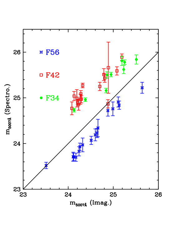
Figure 2: Comparison of the imaging m_5007A magnitude from Hui et al. (1993b ) with the equivalent magnitude computed from the observed [O III]5007Å spectroscopic flux converted to magnitude. The PN in the three fields are shown with different symbols, as indicated.

4.2 Region-averaged PN spectra

Single spectra consisting of the sum of all the observed brighter PN (i.e. those contained in Tab. References) in each of the three fields were constructed. The primary motivation was to enable the detection of fainter diagnostic lines (such as He I, [S II], [Ar IV], etc.) which were not detected, or were marginally detected, on the individual spectra. This was also an explorative study to measure how different the derived abundances would be from the summed spectra in comparison with the ensemble of the individual PN abundances. This aspect is of interest for studies of more distant PN populations where all line detections from individual PN spectra have low S/N and summed spectra are mandatory for measurement of abundances. The radial velocity of each PN was measured from the strong lines in the spectrum (principally [O III] 4959 and 5007Å and H$\alpha$) and employed to shift all the spectra in a single region to zero radial velocity. The spectra were then summed and the resulting emission line spectra fitted in the same way as the individual PN spectra (Section 4.1). Figure 2 of Walsh et al. (Walsh05 (2005)) shows the resulting three spectra. Tab. 5 lists the resulting observed fluxes. The extinction was calculated from the H line ratios with the same assumptions as for the individual PN spectra (Sect. 4.1) and the dereddened line fluxes are listed in Tab. 6.

The ionic abundances of the elements corresponding to the detected species can be determined from the dereddened line ratios with respect to H$\beta$ (Tab. 6). The electron temperature of the O⁺⁺ emitting region can be directly measured from the 5007/4363Å, but also required for abundances is an electron density measure. The only directly determined N_e value is from the [S II]6716/6731Å ratio, which has two disadvantages in that it samples the minority low ionization nebular volume and has a relatively low critical density for collisional de-excitation. Coppeti & Writzel (CoWR02 (1989)) show that [S II] N_e measured in PN is similar to N_e measured for higher ionization species, such as [Cl III] and [Ar IV]. Adopting a value of N_e of 5000 cm^-3 for the NGC 5128 PN appears to be fair and will not lead to bias on the abundance estimates, unless the density is very high (${}^{>}_{\sim}$20 000 cm^-3). In the high density case, the [O III]5007/4363Å line ratio is decreased by collisional de-excitation, leading to too high a value of T_e.

Tab. 7 lists the derived ionic abundances for the summed region spectra. The sources for the atomic data for the collisionally excited lines were taken from the compilation in Liu et al. (Liu2000 (2000)) and the routines from Storey & Hummer (StorHum (1995)) were used for the recombination line emissivities of H and He. The corrections for unseen stages of ionization (ionization correction factors, ICFs) were taken from Kingsburgh & Barlow (KiBa (1994)). The errors in the total abundances do not take into account the errors in the electron temperature; if these are propagated the errors rise to $\pm$0.10 for the O abundance. The He/H abundance is only listed if the lines at 4471 and or 5876Å were detected; if He II 4686Å was detected in addition, it was added to derive the total He/H. If only He II was detected no He/H is listed.

Table 5: Summed PN spectra of three fields in NGC 5128 - Observed line fluxes

		F56		F42		F34
Species	$\lambda$ (Å)	FObs	$\pm$	FObs	$\pm$	FObs	$\pm$
[O II]	3727	28.6	1.7	23.9	2.2	54.5	2.9
[Ne III]	3868	84.0	1.7	62.3	1.5	74.0	1.9
H I	3889	17.3	4.4	13.3	1.6	14.3	1.2
[Ne III] + H$\epsilon$	3970	33.5	1.0	26.9	1.5	34.4	1.9
H$\delta$	4101	21.1	1.2	10.7	1.2	21.3	1.1
H$\gamma$	4340	46.7	1.9	41.5	2.0	40.8	1.5
[O III]	4363	8.7	0.7	6.1	1.3	8.5	0.6
He I	4471	8.0	1.0	6.5	1.0	5.0	3.3
He II	4686	10.7	1.2	9.3	1.9	13.1	1.1
H$\beta$	4861	100.0	0.0	100.0	0.0	100.0	0.0
[O III]	4959	391.3	5.7	396.4	7.1	417.1	7.1
[O III]	5007	1159.6	16.0	1213.6	20.2	1247.8	20.6
He I	5016	3.7	0.4
[N I]	5199	3.2	0.2
He I	5876	14.5	1.9	29.9	5.6
[N II]	6548	50.3	1.2	62.7	4.4	62.7	4.6
H$\alpha$	6562	390.6	3.8	422.7	9.8	412.8	14.7
[N II]	6583	152.2	1.8	149.2	4.3	115.7	5.5
He I	6678	4.6	0.8	7.1	4.6
[S II]	6716	4.5	0.4	7.3	2.8
[S II]	6730	10.9	1.1	27.9	3.0
[Ar III]	7133	28.5	1.1	22.9	3.1
[O II]	7325	27.2	2.4	19.6	4.6
log F(H$\beta$)		-15.46	0.01	-15.42	0.01	-15.78	0.01
m5007A		22.24	0.03	22.10	0.04	22.98	0.04

Table 6: NGC 5128 PN Region spectra - Dereddened line fluxes

		F56		F42		F34
Species	$\lambda$ (Å)	FObs	$\pm$	FObs	$\pm$	FObs	$\pm$
[O II]	3727	37.0	2.3	33.0	3.0	73.8	3.9
[Ne III]	3868	105.9	2.1	83.3	2.1	97.2	2.5
H I	3889	72.0	5.5	17.7	2.1	18.7	1.5
[Ne III] + H$\epsilon$	3970	41.4	1.2	35.0	1.9	44.2	2.4
H$\delta$	4101	25.4	1.4	13.5	1.4	26.4	1.4
H$\gamma$	4340	53.1	1.8	48.7	2.4	47.4	1.7
[O III]	4363	9.8	0.8	6.6	1.3	9.9	0.6
He I	4471	8.9	1.0	7.4	1.2	5.6	3.6
He II	4686	11.2	1.3	9.8	2.0	13.8	1.1
H$\beta$	4861	100.0	0.0	100.0	0.0	100.0	0.0
[O III]	4959	381.8	5.6	384.6	6.9	405.5	6.9
[O III]	5007	1118.3	15.4	1160.0	20.0	1196.3	19.7
He I	5016	3.6	0.4
[N I]	5199	3.0	0.2
He I	5876	11.6	1.5	22.8	4.3
[N II]	6548	36.5	0.9	42.1	2.9	43.0	3.1
H$\alpha$	6562	282.9	2.8	282.8	6.6	282.8	10.1
[N II]	6583	109.9	1.3	99.4	2.9	79.0	3.7
He I	6678	3.3	0.5	4.7	3.0
[S II]	6716	3.2	0.3	4.8	1.8
[S II]	6730	7.7	0.8	18.1	1.9
[Ar III]	7133	19.1	0.8	13.9	1.9
[O II]	7325	17.9	1.6	11.6	2.7
c		0.44	0.03	0.55	0.07	0.51	0.12
log F(H$\beta$)		-15.03	0.01	-14.88	0.01	-15.27	0.01
m5007A		21.18	0.03	20.74	0.04	21.74	0.04

Table 7: NGC 5128 PN Region spectra - Diagnostics and Abundances

Species	F56		F42		F34
	Value	$\pm$	Value	$\pm$	Value	$\pm$
[O III] (5007+4959)/4363Å	153.1	12.6	234.0	46.2	161.8	10.0
[O III] Te (K)	10970	300	9620	560	10780	220
O+	1.76E-5	1.1E-6	2.69E-5	2.4E-6	3.52e-5	1.8E-6
Ne++	7.93E-5	1.6E-6	1.03E-4	2.5E-6	7.28E-5	1.9E-6
He+	0.173	0.019	0.142	0.023	0.109	0.070
He++ (4471Å)	0.0094	0.0011	0.0081	0.0016	0.0115	0.0009
O++	3.091E-4	4.3E-6	4.997E-4	8.6E-6	3.307E-4	5.4E-6
He+ (5876Å)	0.084	0.011	0.160	0.031
N+	1.83E-5	2.2E-7	2.28E-5	6.6E-7	1.32E-5	6.2E-7
S+	4.40E-7	4.6E-8	1.39E-6	1.5E-7
Ar++	1.50E-6	6.3E-8	1.46E-6	2.0E-7
12 + Log(O/H)	8.53	0.01	8.74	0.01	8.59	0.02
He/H	0.182	0.019	0.150	0.023	0.122	0.0070
Ne/O	0.257	0.006	0.206	0.006	0.220	0.007
N/O	1.04	0.07	0.85	0.08	0.38	0.03
12 + log(S/H)	6.55	0.05	7.06	0.04
12 + log (Ar/H)	6.49	0.04	6.44	0.06

4.3 Stellar absorption lines

The slitlets sample a spectroscopic background consisting of sky with a substantial contribution from the galaxy continuum, except for the outermost field, F34. The regions of the slitlets not occupied by planetary nebula spectra can provide the spectrum of the stellar continuum of NGC 5128. The inner fields, F56 and F42, contain no slitlets sampling the sky free of stellar continuum, and so no simultaneous sky subtraction can be performed. For the outer field F34 however, the stellar continuum is very weak and was not detected, as shown by the absence of a gradient in the background with radial offset from the galaxy centre. The 600B F34 spectrum taken on 2003-04-08 was thus used to produce a candidate mean sky spectrum for subtraction from the spectra for the two inner fields (F56 and F42). This sky was interactively subtracted from the F42 and F56 spectra for each slitlet. Good results were found only for the F42 spectra taken in April 2001 and for the F56 field spectra taken in May 2003. These results are attributable to very differing sky contributions to the galaxy spectra at the different observation epochs. For the F56 field, the sky-subtracted data show very low continuum in the five slitlets (1-5) furthest from the galaxy centre; these slitlets were not considered for analysis of the galaxian stellar continuum. Fig. 3 shows the resulting stellar continuum from fields F56 (blue line) and F42 (red line), for all the slitlets summed. Strong CaII H & K, H$\gamma$, H$\beta$ and Mg II lines typical of an intermediate-old stellar population are clearly visible and are indicated on the Figure.

The absorption lines in the individual galaxy continuum spectra for each slitlet were analysed by computing Lick indices (Worthey et al. Worthey (1994)). The spectra were smoothed with a Gaussian to simulate the $\sim$8Å resolution of the Lick/IDS stellar spectra and shifted to zero velocity before the equivalent widths were computed. Errors on the indices were computed by propagating the flux errors in the equivalent width determination. A single radial velocity of 580 kms^-1 was used to shift the spectra to rest wavelength. Errors of $\pm$50 kms^-1 in this radial velocity cause an offset in the bounds of the Lick indices and can introduce errors up to about 0.2Å in EW. Three of the Lick indices (H$\beta$, Mg b and the combined Fe index $<$Fe$>$, defined as 0.5*[EW(Fe_5270A) + EW(Fe_5335A)], are plotted in Fig. 4 as a function of the projected position of the slitlet centres from the centre of the galaxy. The $<$Fe$>$ index shows no radial gradient nor does the H$\beta$ index, although the latter shows higher scatter to larger projected distance from the nucleus. The Mg b index shows a weak negative radial gradient, typical of early type galaxies (c.f. Davies et al. Davies93 (1995)).

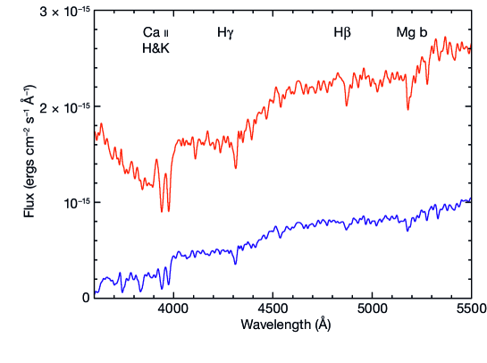
Figure 3: The observed spectra of the galaxy stellar continuum, summed along the whole slit but excluding the positions occupied by the PN, are shown for fields F42 (upper spectrum, in red) and F56 (lower spectrum,in blue). The strongest absorption lines are identified.

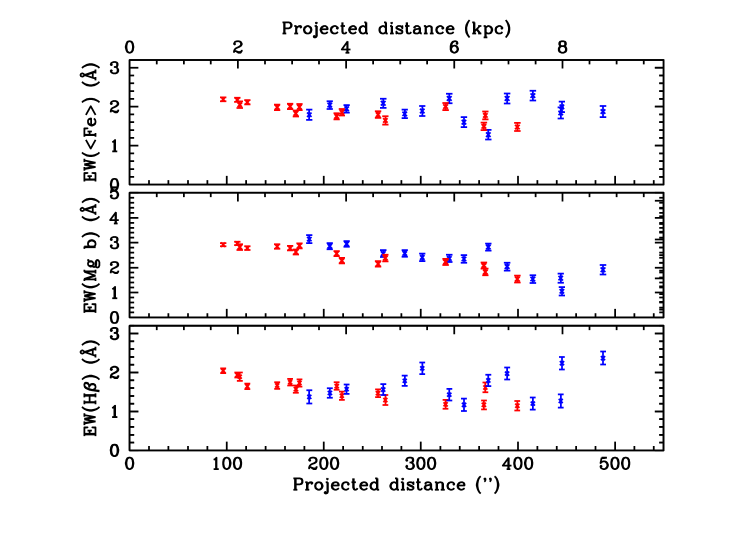
Figure 4: The Lick indices, EW(H$\beta$), EW(Mgb) and $<$Fe$>$ (defined as 0.5*(EW(5270Å) + EW(5335Å)), determined from the stellar continuum in each slitlet, are plotted as a function of the projected distance from the nucleus of NGC 5128, in arcsec (lower axis) and kpc (upper axis). Measurements for field F42 are shown in red and for field F56 in blue.

5 Chemical abundance determination

5.1 Extragalactic PN abundances

The electron temperature (T_e) is required In order to determine reliable chemical abundances for extra-galactic PNe from the collisionally excited lines on account of the exponential dependence of line emissivity with temperature. The electron density (N_e) is also required since these lines have collision cross sections dependent on density. In order to avoid large corrections for unseen ionization species a range of lines of different ionization from neutral and singly ionized up to high ionization is also desirable; however the well-established empirical technique using ICFs can compensate for the lack of some ionization species from the optical wavelength range. As is typical for faint and distant PNe such as observed here, these criteria are not fully met. In the absence of measurements of weak T_e and N_e diagnostic line ratios (such as [O III] 5007/4363Å and [S II]6716/6731Å or [Ar IV]4711/4740Å), the practice adopted by Stasińska et al. (SRM98 (1998)) was to use the upper limits to the strength of these faint lines to constrain T_e and N_e within reasonable limits, taking typical values for PN from studies in the Milky Way and Magellanic Clouds (e.g. T_e $\sim$12000K, N_e $\sim$5000 cm^-3). Jacoby & Ciardullo (JC99 (1999)) introduced a different approach to abundance determination for extra-galactic PNe (in this case for M31): that of photoionization modelling using the very well-established Cloudy (Ferland et al. Ferland (1998)) code. The gains of this latter method are that both strong lines with low errors, weak lines with large errors and upper limits can all be used in arriving at a satisfactory model, and the parameters of the central stars (luminosity, $\cal L$ and effective temperature, $T_{eff}$) are derived as part of the photoionization modelling.

Extra-galactic PNe are spatially unresolved but have known distances and absolute fluxes available though m_5007Å photometry. An input data set for photoionization modelling can be assembled, given some simplifying assumptions in the absence of more detailed information; in particular, the nebular geometry and information on the stellar atmosphere are not available. A black body has been shown to be an acceptable assumption for PN central stars (Howard et al. Howard97 (1997)), which leaves the nebular geometry. Taking a spherical shell of constant density as a baseline, Jacoby & Ciardullo (JC99 (1999)), hereafter JC99, compared nebular abundances using directly measured T_e and N_e values and ICFs to check that photoionization modelling was indeed a valid approach. The approach was shown to work well. Additional complexity, such as two zone density structure and the presence of dust within the nebula, was found to be required to satisfactorily match the observed spectra in some cases.

Magrini et al. (Magrini (2004)) followed the same procedure as JC99 in determining abundances of PNe in M33. They also tested the method by applying it to the integrated spectra of well-observed Milky Way PNe and compared the model abundances to those from the ICF method, finding agreement within 0.15 dex for O/H and 0.3 dex for N/H. In addition Magrini et al. (Magrini (2004)) compared abundances derived from Cloudy models with those from ICFs for three PNe of their M33 sample. They also considered comparisons employing model atmospheres and an $r^{-2}$ density in the nebular shell, and found no major discrepancies. The technique, involving the development of a large number of models in working to a satisfactory match of observed and model spectrum, is labour-intensive and therefore not suitable for large samples. It also requires simplifying assumptions. The technique, however, is well suited to the present sample of PN spectra in NGC 5128 where the range of abundances is of particular interest and the data set is limited; it also serves as a probe of the star formation history.

Only 10 of the PN spectra presented in Tables References and References have detectable [O III]4363Å, enabling direct measurement of the electron temperature, and only 7 have an electron density sensitive ratio ([S II]6716/6731Å) measured. The typical S/N on the weak 4363Å line ($\leq 3$) implies that T_e errors of 1250K at 11000K affect abundance determination, leading to errors of ${}^{+0.17}_{-0.13}$ on log (O⁺⁺/H⁺). For the PNe without detectable diagnostic line ratios, two approaches are possible: employ the region-averaged spectra to assign T_e and N_e values to the single PN, although these values may be substantially in error for particular nebulae; or, employ photoionization modelling of the strong lines to find the best-matching model that does not violate the upper limit constraints for the weak lines.

5.2 Modelling procedure

The simplest possible photoionization model was employed: a black body central star characterized by its temperature and luminosity, the latter given by the H$\beta$ luminosity derived from the m_5007Å magnitude (Hui et al. 1993b ), the reddening and the dereddened 5007Å/H$\beta$; a spherical shell with the inner radius set to a small value (0.005 pc) to ensure high ionization emission close to the central star, but not so close that instabilities arise in the model; the outer radius set to a large value (0.5 pc) since the nebulae are expected to be optically thick, as given the high luminosity of the PNe observed in NGC 5128 (i.e. within 2 mag. of the peak of the PNLF); and an initial set of abundances. For the abundances of He, N, O, Ne, S and Ar, the initial values were taken from the ICF analysis for the integrated spectra listed in Tab. 8 and the C/O ratio taken as 0.5. However these values were immediately allowed to vary to fit the individual spectra (with C varying in lock-step with O) and should not be seen as prejudicing the individual determinations from the higher S/N integrated spectra. The initial assumption of an optically thick nebula could also have been relaxed in the modelling process but was not found to be demanded by the fits to the PN spectra. The philosophy was to aim to match the dereddened lines fluxes within the listed errors for all the spectra listed in Tab. References (except F56#9, F56#17, F42#15b and F42#17 without detected [O II] or He lines), thus 40 PN spectra. These PNe represent the upper 2.1 mag. of the PNLF.

The modelling procedure followed closely that outlined by JC99 and also Marigo et al. Marigo (2004). An initial default density of 5000cm^-3 was used. The initial estimate of $T_{eff}$ was taken from He II 4686Å/H$\beta$; in the absence of 4686Å, its upper limit and the 5007Å/H$\beta$ ratio was used. The presence of 4686Å enabled $T_{eff}$ to be refined within a few runs of Cloudy; if 4686Å was not present, both $T_{eff}$ and O/H had to be adjusted. Then He was adjusted to match the He I lines, with minor adjustments to T_e for the concomitant changes in He II flux. O/H and the density were adjusted to match [O II]3727Å and, if present, the [O II]7325Å quadruplet. For large changes in O abundance, Ne and C were initially changed in proportion. Once the basic physical parameters ($T_{eff}$, density, He, O) were roughly determined, Ne, N, Ar and S were altered to match the observed lines. In the final phase all lines and $T_{eff}$ and density were subject to small changes to improve the fit, where possible. A guide to the goodness of fit of the observed and predicted line strengths was formed, taking the sum of the line flux differences normalised by the S/N: thus larger discrepancies for weak lines could be weighted lower. A discussion of the goodness of the matches and the estimation of errors in presented in section 5.4. In general around 10 iterations per PN was enough to reach a satisfactory match to the spectrum but in more difficult cases (F56#12b, F42#10 and F34#7 for example) up to 30 iterations were required. In total, $\sim$600 Cloudy models were run to complete this analysis.

Table 8: Cloudy photoionization modelling of 40 PN in NGC 5128

PN #	Elemental Abundances 12 + log(A/H)						Teff	Log $L$	Ne	Quality3
	(He/H)	(N/H)	(O/H)	(Ne/H)	(S/H)1	(Ar/H)2	(kK)	($L_{\odot}$)	(cm-3)
F56#1	11.06	8.20	8.40	7.70	6.55	6.00	60	3.68	5000	b
F56#2	11.15	7.85	8.43	7.72		6.00	155	4.20	10000	a
F56#3	11.06	8.30	8.48	7.78	6.55	6.00	64	3.66	2000	b
F56#4	11.06	8.30	8.38	7.70	6.55	6.50	78	3.75	5000	b
F56#5	11.06	7.40	8.55	7.85		6.35	150	3.74	10000	c
F56#6	11.20	8.30	8.64	7.95		6.60	75	4.15	6000	b
F56#8	11.20	8.62	8.60	7.80	6.80	6.50	63	3.77	9000	b
F56#10	11.10	8.20	8.38	7.60	6.55	6.60	88	4.03	15000	b
F56#11	10.90	8.42	8.54	7.70	7.00	6.40	90	3.67	22500	a
F56#12a	11.10	8.53	8.80	8.10	6.55	6.40	200	3.86	10000	a
F56#12b	11.00	8.80	8.55	7.85		6.50	45	3.93	35000	b
F56#13b	11.00	7.60	8.52	7.70		6.20	105	3.76	20000	a
F56#14	11.06	8.40	8.46	7.70	6.55	6.30	95	3.86	15000	b
F56#15	11.06	7.90	8.47	7.70	6.55	6.20	70	3.86	10000	c
F56#16	11.06	8.20	8.47	7.60	6.55	6.20	70	3.91	10000	b
F56#18	11.06	8.63	8.51	7.85	6.90		90	3.87	15000	b
F42#1	11.12	7.85	8.45	7.65	6.90	6.20	80	3.83	10000	c
F42#2	11.06	8.19	8.68	8.03			155	4.05	10000	a
F42#3	11.06	8.26	8.44	7.50		6.40	50	3.99	10000	c
F42#4	11.01	8.12	8.03	7.10	6.40	6.20	86	4.00	12000	a
F42#6	11.15	7.30	8.44	7.60	7.10		63	3.63	13000	b
F42#7	11.06	8.00	8.51	7.70			127	3.64	10000	b
F42#8	11.06	8.20	8.46	7.70			93	3.86	15000	b
F42#9	11.12	8.20	8.45	7.70		6.50	74	3.78	30000	b
F42#10	11.28	8.18	8.10	7.40	6.85	6.10	120	4.29	2500	a
F42#11	11.06	8.25	8.28	7.35	6.85	6.20	100	3.72	10000	c
F42#12b	11.06	8.22	8.69	8.07			108	4.09	10000	b
F42#13	11.06	8.28	8.90	8.25			190	3.84	16000	a
F42#14b	11.06	8.20	9.00	8.40	6.70		220	4.06	20000	a
F42#16a	11.06	8.28	8.72	7.92			100	3.78	14000	a
F42-18	11.06	7.68	8.49	7.45			120	4.35	10000	c
F34#1	11.06	8.25	8.73	8.00		5.65	71	3.89	8500	a
F34#2	11.23	7.62	8.09	7.38			90	4.11	1500	a
F34#4	11.06	8.10	8.46	7.70		6.30	67	3.90	8000	b
F34#7	11.06	8.30	8.91	8.30		6.50	82	3.99	13000	a
F34#11	11.16	7.40	8.53	7.78			180	3.59	30000	a
F34#12	11.16	7.35	8.48	7.30			167	3.13	30000	a
F34#14	11.06	7.90	8.62	7.82			70	3.61	20000	b
F34#15	11.06	7.40	8.43	7.76			123	3.90	10000	b
F34#16	11.06	8.28	8.63	7.95	6.55		180	3.70	5000	a

5.3 Results and scrutiny

Tab. 8 lists the derived abundances for He, N, O, Ne, Ar, and S with respect to H where lines of these elements were detected, together with the stellar luminosity, black body temperature and the constant shell density. The quality of the derived parameters are broadly classified into three categories based on: He II (and or [O III]4363Å) and [O II] both detected (15 PN: grade a); [O II] but not He II detected (18 PN: grade b); neither He II nor [O II], but at least He I, [O III]5007Å, [Ne III]3868Å and [N II]6583Å, detected (6 PN: grade c). Ten of the quality “a” spectra had 4363Å detected and the models tailored to fit the strong lines (i.e. a model was not tweaked to exactly fit the 4363Å line) were found to match the 4363Å line within the $1\sigma$ errors in all cases except one (F42#16a; 4207 in Hui et al. 1993b ). The results presented are not claimed to be unique, as the adopted geometry of the nebulae is the simplest possible and the use of a black body atmosphere does not produce the most satisfactory fits to the level of ionization in detailed photoionization modelling of Galactic PNe (e.g. Wright et al. Wright (2011)). However these simple models are capable of matching the observed variety of spectra with a very plausible range of abundances, central star temperatures and nebular densities.

Carbon is the most important coolant after O, but no lines of C were detected so there are no direct constraints on the C/H abundance. In the absence of other evidence, the abundance of C was assumed to be similar to O (C/O=0.5) and to vary in lock-step with O as the abundance of O was altered to match the spectrum. Once an adequate model had been found, tests were performed on four of the spectra, altering the C abundance by a factor 2.5 and refitting for the other species. A maximum difference in 12+log(O/H) of -0.10 was found for 12+log(C/H) higher by +0.40; for 12+log(C/H) lower by 0.40, a maximum difference of +0.02 in 12+log(O/H) was found. Smaller changes in N and Ne abundances were required to match the spectra with these altered C abundances. Thus the abundances are not very sensitive to modest changes in the assumed C/O ratio.

For the best observed PN spectrum (viz. the target with the brightest m_5007Å) PN, (F56#2; 5601 in Hui et al. 1993b ), a set of Cloudy models were run with NLTE model atmospheres from the Tübingen compilation (Rauch Rauch03 (2003)), and also with the presence of dust inside the ionized region. H, He and PG1159 model atmospheres were employed. While the H model atmosphere showed a much lower $T_{eff}$, an He or PG1159 atmosphere at 170-180 kK produced satisfactory fits, with the resulting O/H lower by up to 0.16 dex. Including dust with an atmosphere model required that O/H be reduced by up to 0.05 for a gas-to-dust mass ratio of 1000; as the primary coolant of the nebula, the lower O/H is compensated by the enhanced cooling from dust.

Stasińska (Stas2002 (2002)) questioned the uniqueness of abundance determinations even in the case that a direct measure of T_e from e.g. [O III]4363Å is available. Depending on the temperature of the central star, a strong gradient in the electron temperature can exist within the nebula and a single value of T_e may not be a good representation for the bulk of the emission. The T_e gradient is far less steep for PNe with hot central stars ($\sim$100 000K) than for cooler central stars and the use of a single T_e should yield reliable abundances. Stasińska (Stas2002 (2002)) presented photoionization models for a Milky Way Bulge PN with a central star temperature of 39 000K that can be equally well fit by a lower abundance ([O/H]=-0.31) and by a higher abundance model ([O/H]=+0.39). 95% of the PNe observed in NGC 5128 appear to have $T_{eff}\geq$ 60kK, so the likelihood of a double-valued abundance is very low. However since the lowest $T_{eff}$ values derived in the Cloudy modelling (Tab. 7) are $\sim$50kK, then uniqueness may be a more significant concern for these few objects.

A concerted attempt was made to fit the spectra of the PNe with the lowest derived T_eff by low and high metallicity (Z) models. Here there is the liberty to change the stellar temperature since the He II 4686/H$\beta$ ratio can be taken as an upper limit based on the errors on local lines. Two PN were found that could not be distinguished in terms of lower and higher Z Cloudy models. In the case of F56#12b (a class b spectrum with the [O II] line detected but not He II), the higher Z solution with 12+log(O/H) of 8.55 for a BB $T_{eff}$ of 49 kK could not be distinguished from a model with $T_{eff}$ of 73 kK and 12+log(O/H) of 8.06 if the density was decreased from $4.0\times 10^{4}$ to $1.8\times 10^{4}$ cm^-3. For F42#3 (class c spectrum without [O II] and He II lines detected), a higher Z solution with 12+log(O/H) of 8.44 for $T_{eff}$ of 50 kK was indistinguishable from that with 12+log(O/H) of 8.01 but $T_{eff}$ of 73kK, for the same density in the shell. For the class c PN, an attempt was made to match each spectrum by a forced lower Z model but no convincing matches could be found; nevertheless, one may exist given the rather weak constraints implied by these lower quality spectra. Conservatively, the higher abundance solutions were adopted (in Tab. 8) on the grounds that they do not differ strongly from the values for other PNe at similar radii.

The two PNe with alternate low O/H values are not improbable and are comparable to the abundances of PNe in dwarf galaxies (e.g. Dopita & Meatheringham, Dopita91 (1991) and Leisy & Dennefeld, Leisy06 (2006)); F42#4 also shows a similarly low value of O/H but has a well-detected spectrum. In the context of a giant elliptical galaxy, such low abundance values are surprizing because they imply low metallicity progenitor stars,. Radial velocities of these PNe (available for F56#12b and F42#4 from Peng et al. Peng04 (2004)) do not show ’peculiar’ velocities, being within 1$\sigma$ of the mean velocity of NGC 5128. There is no indication of these PNe being obvious ’halo’ objects or of resulting from a recent low-mass galaxy interloper not yet in dynamical equilibrium with the parent galaxy.

The abundances of the individual PN from Tab. 8 were combined and compared to the abundances derived from the integrated region spectra with empirically determined temperatures and ICFs presented in Tab. 7. The means were determined by weighting the individual abundances by m_5007A. For the combined region F56, the weighted mean abundances from Tab. 8 for O agreed to within 0.01 dex and for F34 to within 0.06 dex (weighted means of the log and the fractional O/H abundances were calculated with similar results). For field F42, the discrepancy on the weighted mean of the log O abundance was larger, with a value up to 0.22 dex lower than the value in Tab. 7. The difference for F42 is quite striking in this comparison; the electron temperature was measured to be $\sim$1 000K lower than for the other two regions. It is suggested that the value of T_e was underestimated in this merged spectrum due to a poorly determined [O III]4363Å flux.

A further check on the integrated region spectra was performed by running photoionization models for the region spectra presented in Tab. 6. The abundances were compared to the empirical abundances derived using ICFs (Tab. 7). Satisfactory Cloudy models could not be fitted without departing from the simplifying assumptions used for the individual PN models. In particular, when the stellar temperature was chosen from the He II/H$\beta$ ratio, this could not be made compatible with the electron temperature derived from the [O III]5007/4363Å ratio. If He II4686Å matched the observations within the errors, then [O III]4363Å was predicted much too strong (higher T_e); when [O III]4363Å matched the model, He II was modelled too low (lower $T_{eff}$). The addition of modest amounts of dust inside the ionized region of the photoionization model to provide extra heating through photoelectric emission from the grains did not resolve this discrepancy. However allowing for these modelling issues, the range of O/H was close (within 0.1 dex) to the empirical values listed in Tab. 7 for the sum of PNe in fields F56 and F34, but only within 0.2 dex for F42. These demonstrations show that summing PN spectra provides a useful indicator of the mean O abundance in cases when the line detections have low S/N, such as for PNe in more distant galaxies. This conclusion is subject to the condition that the PN abundances do not differ strongly, as in this case. Méndez et al. (Mendez05 (2005)) have presented lower limits on O and Ne abundances based on just such a summed spectrum for 14 PNe in NGC 4697 (an elliptical at 11 Mpc).

5.4 Towards a comparative study of models

A number of Cloudy photoionization models were run in order to arrive at an adopted model for each PN matched in Tab. 8. The models presented cannot be claimed to be unique but represent a feasible match to the spectra in terms of the abundances and physical conditions within the restricted set of parameters (black body atmosphere for the stars, linear density law, etc). Magrini et al. (Magrini (2004)) and JC99 discussed the accuracy of photoionization models to their PN spectra. In general the “a” quality spectra of the NGC 5128 PN approach those of the fainter sample of the much closer PNe observed in M33 and M31 by these authors. Simply adopting the range of models within the statistical errors on the line ratios underestimates the real uncertainties on the abundance determinations. For a selection of models, independent Cloudy runs were performed by two of the authors and the results compared (c.f. Jacoby et al. Jacoby97 (1997)) and with the ICF determinations in the cases where [O III]4363Å was detected (using an adopted N_e value of 5000 cm^-3). While a full error analysis is outside the scope of this work, a limited investigation was attempted. A range of parameter values around the adopted ones were explored to determine the sensitivity of the models, given the errors on the spectra.

It would be very time consuming to perform an investigation of the likely parameter range for all PN in Tab. 8, so two PN were selected. F56#2 was chosen as a high S/N case with both [O III] 4363Å and He II 4686Å well detected (a class “a” spectrum in Table 8) and a high stellar temperature. F34#1 was chosen as a PN with lower S/N and only a marginal detection of He II 4686Å (class “b” in Table 8) and a lower stellar temperature and representing the typical average quality of spectra. Cloudy models were run for these two exemplars varying a number of parameters about the adopted solution in Tab. 8: O abundance varied by $\pm$0.2 dex; stellar black body temperature by 10-15% (20 000K for F56#2, with $T_{BB}$ 155 000K and 10 000 K for F34#1, with $T_{BB}$ 71 000 K); the density by a factor of two; and a model atmosphere rather than a black body. For each modified parameter set, Cloudy models were run to match the spectra within errors as far as possible by freely varying all the other, non-displaced, parameters. Even this limited analysis involved running more than 180 separate Cloudy models.

The results of the comparison of Cloudy models are summarised in Tables 9 and 10. The third columns list the dereddened spectrum from Tab. References and the 4th column the spectrum resulting from the adopted model given in Tab. 8. The successive columns list the resulting spectra from the incremented parameters. The lower half of each table lists the stellar temperature, density and abundances corresponding to the spectrum in the upper part of the same column; values in column 4 being identical to those in Tab. 8. An overall merit factor, $FoM$, of the match of the model spectrum with the observed spectrum, taking account of the S/N of the fluxes, is defined by:

$$FoM=\sum_{i=1}^{n}|((F_{obs}-F_{mod})/F_{obs})|\times(F_{obs}/Err_{obs}))$$ (1)

where $F_{obs}$ and $Err_{obs}$ are respectively the dereddened flux and error and $F_{mod}$ the model flux; the summation is taken over the number of emission lines. Since some lines are in fixed ratio, such as H lines, a subset of the lines was adopted to dispense with some redundant information (except for the more important lines such as H$\alpha$ and H$\beta$, the weak He I lines and the [O III] 4959Å line).

Table 9 presents the comparative models for the bright PN F56#2 (5601 in Hui et al. 1993a ). The comparison of the observed and model spectra makes it clear that the He I 5876Å line is strongly under-estimated, most probably because of the poor removal of the strong Na I telluric emission. In general satisfactory models could be found, except for the cases of O - 0.2 abundance (column 6 of Table 9) and $T_{BB}$ - 20 000 K (column 8). What constituted a satisfactory match to the spectrum was not simply given by the FoM value, but certain line ratios, which act as important diagnostics of nebular conditions, e.g. He II/H$\beta$, [O III] 5007Å/H$\beta$ and [O III] 5007/4363Å), were given higher weight in assessing the quality of the match. It is clear that a range of O $\pm$0.2 produces model spectra in which the important [O III] lines are not well-matched, and thus representative errors on O in the range 0.1 to 0.15 are suggested. Similarly the range of stellar temperature of $\pm$20 000 K and density varying by a factor 2 also over-estimate the allowed range of some of the line ratios. However it is clear from these parameter ranges that the error bars are not necessarily symmetric. H, He and PG1159 atmospheres from Rauch et al. Rauch03 (2003) were input to Cloudy and although the choice of temperatures is not very extensive, a satisfactory fit with the PG1159 atmosphere for 170 000 K was found. However this should not be considered as a best estimate since a comprehensive range of temperature and gravity was not tested.

The comparative models for the fainter PN F34#1 (2906 in Hui et al. 1993a , $m_{5007A}$=24.96) are given in Tab. 10. Here the number of lines is less than F56#2, since [O III]4363Å  and no He I lines were detected and He II is a limit. The [O II] 7325Å line is clearly under-estimated in the measured spectrum by comparison with the model spectra. Satisfactory matches could generally be obtained with the ranges of parameters listed. The models with a range of O of $\pm$0.2 is clearly accommodated by the data. Only the lowering of the stellar temperature by 10 000 K (column 8 of 10) produced an unsatisfactory fit. A PG1159 model atmosphere (Rauch Rauch03 (2003)) of 70 000K produced a good fit (column 11), but the 70 000 K He model produced a similar fit with an O abundance lower by 0.40 dex than the black body.

From this comparison of observed and model spectra with a higher and a lower S/N, we conclude that the typical dependence of errors on the choice of Cloudy models are generally in the range of 0.15 - 0.20 for the O abundance, around 10-15% for He and around 0.2 for Ne and N. These values are similar to those found by Magrini et al. Magrini (2004) comparing abundances from Cloudy models with those of the ICF method. These representative abundance errors are shown in plots, such as Figs. 6 and 7.

Table 9: Comparative Cloudy photoionization modelling of F56#2

Species	$\lambda$ (Å)	Flux &	Model	Model	Model	Model	Model	Model	Model	Model
		error		O + 0.2	O - 0.2	TBB + 20 kK	TBB - 20 kK	Ne $\times$ 2.0	Ne $\times$ 0.5	Mod.atmos.
[O II]	3727	56 $\pm$ 13	59	58	47	53	59	32	53	57
[Ne III]	3868	124 $\pm$ 13	124	127	128	122	123	126	125	125
[O III]	4363	28 $\pm$  8	24	15	27	26	22	22	22	27
He I	4471	6 $\pm$  3	6	6	6	3	11	6	9	6
He II	4686	39 $\pm$  8	39	38	34	46	30	37	30	38
H$\beta$	4861	100 $\pm$  0	100	100	100	100	100	100	100	100
[O III]	4959	457 $\pm$ 31	449	448	398	451	471	454	458	456
[O III]	5007	1367 $\pm$ 90	1350	1348	1199	1358	1417	1367	1377	1371
He I	5876	6 $\pm$  3	18	18	19	11	33	19	28	20
H$\alpha$	6562	281 $\pm$ 19	286	285	290	286	286	284	285	288
[N II]	6583	55 $\pm$  5	54	57	58	53	53	54	53	57
He I	6678	7 $\pm$  4	4	5	4	2	8	4	7	5
[Ar III]	7133	8 $\pm$  3	9	6	10	8	9	7	9	8
[O II]	7325	14 $\pm$  4	16	14	13	19	14	15	9	16
Model input
TBB(kK)			155	152.5	150	175	135	150	132.5	1701
NH (cm-3)			10000	10000	10000	12000	8000	20000	5000	10000
12+log(He)			11.15	11.15	11.20	11.00	11.35	11.15	11.30	11.18
12+log(C)			8.40	9.20	6.60	8.40	8.40	8.70	8.40	8.20
12+log(N)			7.85	8.02	7.84	7.85	7.88	8.01	8.05	7.85
12+log(O)			8.43	8.63	8.23	8.48	8.43	8.49	8.40	8.39
12+log(Ne)			7.72	7.96	7.57	7.75	7.70	7.78	7.70	7.67
12+log(Ar)			6.00	6.00	6.15	6.00	6.00	6.00	6.00	5.95
FoM			7.53	8.30	13.46	7.34	14.79	9.06	12.90	8.56

Table 10: Comparative Cloudy photoionization modelling of F34#1

Species	$\lambda$ (Å)	Flux &	Model	Model	Model	Model	Model	Model	Model	Model
		error		O + 0.2	O - 0.2	TBB + 10 kK	TBB - 10 kK	Ne $\times$ 2.0	Ne $\times$ 0.5	Mod.atmos.
[O II]	3727	86 $\pm$  9	89	85	88	87	60	49	144	85
[Ne III]	3868	93 $\pm$  6	91	92	93	92	95	92	94	96
He II	4686	2 $\pm$  2	2	2	4	4	1	2	4	0
H$\beta$	4861	100 $\pm$  0	100	100	100	100	100	100	100	100
[O III]	4959	393 $\pm$ 15	384	391	384	393	248	385	387	390
[O III]	5007	1164 $\pm$ 41	1156	1177	1157	1183	747	1157	1166	1174
H$\alpha$	6562	283 $\pm$ 12	288	290	287	286	286	287	288	287
[N II]	6583	104 $\pm$  6	104	104	104	104	103	104	105	103
[Ar III]	7133	4 $\pm$  3	3	4	4	4	3	3	4	4
[O II]	7325	4 $\pm$  3	17	16	17	17	8	16	17	14
Model input
TBB(kK)			71	68	78	81	61	67.5	80	701
NH (cm-3)			8500	10000	7500	8500	8500	17000	4250	7000
12+log(He/H)			11.06	11.06	11.06	10.90	11.30	11.06	10.90	11.20
12+log(C)			8.60	8.50	8.40	8.80	8.50	8.60	8.30	8.20
12+log(N)			8.25	8.38	8.13	8.16	8.50	8.40	8.03	8.18
12+log(O)			8.73	8.93	8.53	8.60	9.00	8.78	8.54	8.60
12+log(Ne)			8.00	8.23	7.78	7.84	8.60	8.07	7.77	7.88
12+log(Ar)			5.65	5.85	5.55	5.60	5.90	6.65	5.55	5.60
FoM			6.44	5.79	6.48	6.74	26.62	10.20	12.90	5.30

6 Discussion

6.1 Individual PN spectra and abundances

A sample of 51 PNe in NGC 5128 have been observed over a range of projected galactocentric distances from 1.7 to 18.9 kpc and covering the PN luminosity function from the brightest known PN in NGC 5128 (PN 5601, $m_{5007A}=23.51$) to 4.1 mags fainter. The mean 5007Å/H$\beta$ ratio is 11.00 $\pm$ 0.55 (r.m.s on the mean) for the 42 spectra with the highest S/N. The extrema of the 5007Å/H$\beta$ values for this subset are 6.0 ($\pm$ 0.67) to 18.8 ($\pm$3.7); the value of this ratio is very sensitive to the subtraction of the underlying continuum and the variation of the H$\beta$ absorption line along the slitlet. The mean logarithmic extinction correction at H$\beta$ is 0.56 $\pm$ 0.20. The overall Galactic extinction to NGC 5128 is E_B-V=0.123 (Burstein & Heiles BurHei (1984)) or E_B-V=0.115 (Schlegel et al Schlegel (1998)), the latter is equivalent to c=0.17 for a Galactic extinction law with R=3.2 (Seaton Seaton (1979)). The lowest values of extinction measured in the PNe (Tab. References) are compatible with no local extinction in NGC 5128. The histogram of c values peaks at 0.45 ($E_{B-V}$ = 0.30) and shows no obvious trend with radial offset beyond 200^′′ from the nucleus; the five highest values occur within a radius of 200^′′ (3.7 kpc). The frequency of higher c values at lower radii is probably due to the high line of sight extinction in the vicinity of the dust lane, rather than any intrinsic PN property (e.g. high intrinsic dust content associated with young PNe, such as NGC 7027; Zhang et al. Zhang (2005)).

The ratio of 5007Å/H$\beta$ does not show any significant overall gradient with projected radial offset from the galaxy centre; the highest values lie in field F42 where the stellar continuum is strongest and removal of the underlying H$\beta$ is the most critical. There is no evidence for a gradient in [Ne III]/[O III] implying a constant O⁺⁺/Ne⁺⁺ ratio. If there is any O enrichment, e.g. during the third dredge-up (Péquignot et al. Pequ (2000)), or depletion (through the ON cycle, Leisy & Dennefeld Leisy06 (2006)) occurring in the nebular envelopes of the PNe, then this constant value of the ionic ratio implies that any alteration in O abundance must be accompanied by a corresponding change in Ne. Since O-Ne correlation is not predicted by AGB evolution (Karakas & Lattanzio KarLat (2003)), the rather constant O/Ne ratio implies that O enrichment/depletion is not an important effect.

The mean 12 + log(O/H) is 8.52 $\pm$ 0.03 (median value 8.48) and the range of [O/H] is $-$0.66 to $+$0.31. The mean O/H abundances inside and outside 10 kpc are identical. Of the three PN with the lowest O/H, two occur close to the nucleus (F42#4 and F42#10) and the other is at 19.5 kpc (F34#2) and all have low [O III]/H$\beta$, without notably strong [O II]; F34#2 has lower N/H. The PN with the highest O/H occur in fields 42 and 56 and are distinguished by very high [O III]5007/H$\beta$ but with large errors. The problems in removing the underlying stellar continuum from slit measurements can contribute to large uncertainty on the line fluxes for fainter nebulae in the central regions (see the discussion in Roth (Roth06 (2006))), and very high [O III]/H$\beta$ of $>$ 15 must be viewed with caution since the H$\beta$ may be considerably underestimated.

The mean N/O ratio is 0.51 $\pm$ 0.06. Four PNe were found with high N/O ratio (F56#8, F56#12b, F56#18 and F42#4) but only F56#12b and F56#18 have He/H and N/O which could be classified as characteristic of Type I nebulae (Peimbert Peimbert (1978)). Since F56#12b was modelled by a lower temperature central star (the lowest of all the PN modelled, Tab. 8), it may be that optical depth effects and the assumption of a black body may yield misleading results. F56#18 is perhaps a better candidate for a Type I nebula, having a relatively high stellar temperature and a higher reddening, but this PN does not possess the highest luminosity central star. The brightest PN, and incidentally the nebula with the highest luminosity star (Tab. 8), has N/O of 0.12 and shows no elevation of this ratio, compared for example to the mean Milky Way value of 0.47 (Kingsburgh & Barlow KiBa (1994)). The shorter timescales for PN evolution of Type I PN make them minor contributors to a PN population luminosity function, but they contribute about $\sim$10% of Milky Way PN by number.

The mean oxygen abundances in NGC 5128 PNe are intermediate between values for the LMC (12 + log(O/H) mean 8.4 (e.g. Leisy & DennefeldLeisy06 (2006)), and that of the Milky Way (mean 8.68, Kingsburgh & Barlow KiBa (1994)). A plot of the dependence of the [O III]5007Å luminosity on 12+log(O/H) (Fig. 5) shows a tendency to increase with the oxygen abundance, in line with the theoretical relation of of Dopita et al. (DopJac (1992)) as observationally transformed by Richer (Rich93 (1993); see Figure 2 and equation 1). A second order fit to the observed points demonstrates a comparable dependence of [O III] luminosity on (O/H) to the theoretical relation and is shown in Fig. 5 by a dashed line.

Figure 5: The dependence of the oxygen abundance of the NGC 5128 PN sample from the Cloudy photoionization modelling (Tab. 8) on the observed [O III] 5007Å luminosity (uncorrected for reddening) from the 5007Å photometry of Hui et al. 1993b . The dotted line shows the theoretical relation of Dopita et al. (DopJac (1992)) scaled to the brightest PN, while the dashed line shows a second order polynomial fit to all the data points.

The region summed spectra provide good detections of a single ionization species of S and Ar (Tab. 6) and lines of these species were detected in a number of the brightest PNe (Tab. References and References) allowing useful indications of S/H and Ar/H (Tab. 7 and Tab. 8). S and Ar abundances serve an important purpose in that they are not considered to be affected by the AGB nucleosynthesis (e.g. Herwig Herwig (2005)). Whilst O is the element which is most easily measured in PN since it is the dominant coolant, it can be destroyed by CNO cycling or synthesized during helium burning which impacts its usefulness as a metallicity indicator. Péquignot et al. (Pequ (2000)) have found evidence for third dredge-up O enhancement in a PN in the Sagittarius dwarf galaxy (12+log(O/H) = 8.36), but only at the level of $<$0.03 dex. By comparing the lock-step dependence of Ne and O in PN samples, Richer & McCall (Rich08 (2008)) conclude, in agreement with Karakas & Lattanzio (KarLat (2003)), that the majority of PNe do not show any changes in the O or Ne abundances across the AGB and PN transition. The Ne/H abundances are well correlated with the O abundances for the NGC 5128 PNe as shown by Fig. 6 (slope 1.22$\pm$0.09, or 1.17$\pm$0.04 excluding the 4 points furthest from the linear relation) This result is similar to the value found by Leisy & Dennefeld (Leisy06 (2006)) for the LMC (slope 1.13). The relation between N/O and O/H is also shown in Fig. 6. There is considerable scatter with a weak but insignificant trend for an anti-correlation, as also found by Magrini et al. Magrini (2004) for PNe in M33. The mean Ar/H abundance (6.3 for 21 PNe) is indistinguishable from the mean for 70 PN in the Milky Way (Kingsburgh & Barlow KiBa (1994)). The mean S abundance (6.8 for 9 PNe) also appears to be similar to the mean value from the Kingsburgh & Barlow (KiBa (1994)) sample. One is led to the surprising conclusion that most of the PN abundances in NGC 5128 are not significantly different from the mean values for Milky Way PNe.

Figure 6: The relationship between log (Ne/H) and log (O/H) is shown (upper) and for Log(N/O) against log (O/H) (lower) for the individual NGC 5128 PN abundances tabulated in Tab. 8. The representative error bars are indicated.

6.2 PN 5601

PN 5601 (F56#2) is the brightest known PN and the best-studied individual PN in NGC 5128, and indeed of all PN known beyond the Local Group. Walsh et al. (Walsh99 (1999)) measured long slit observations of this PN amongst a few others and the major difference between the spectrum presented in Tab. References is the H$\alpha$/H$\beta$ ratio and the higher He II/H$\beta$ ratio. The earlier observations were taken with a fixed slit position angle over a considerable range of parallactic angle and suffer from wavelength dependent flux loss from the slit. This is demonstrated by the very low value of extinction derived. The value of extinction derived for this nebula is now seen to be quite large, but only slightly higher than the mean value for all the observed PN (E_B-V=0.32), giving no evidence that it is intrinsically dustier than the fainter PNe. There is some expectation from examples of Milky Way PNe, that young, high mass, optically thick PN (c.f. NGC 7027, Zhang et al. Zhang (2005); NGC 6302 Wright et al. Wright (2011)) have higher intrinsic dust extinction.

6.3 Abundance gradient from PNe

One of the primary aims of this study was to investigate any abundance gradient of the $\alpha$-elements, as revealed by the PN spectra, and to compare it to gradients in the stellar properties such as the metallicity distribution function. A plot of the variation of O/H v. projected radial offset (Fig. 7), for the PNe with O/H values from the Cloudy models (Tab. 8), shows two particular features. First, the range of O/H values is similar in the inner regions (projected radius, $\cal R$ $<$4 kpc) to the range in the outer regions ($>$13 kpc). Second, there is no evidence of a gradient in O/H. A least squares fit confirms this; the linear correlation coefficient is -0.07 for 40 points. Rather, there is a common mean value of 8.52 for the inner and outer points (considered as less than and greater than $\cal R$ of 10 kpc). However, the highest O/H values do occur at $\cal R$ $<$ 4 kpc, in the inner field F42. Although our sample is not large, the result that there is no significant O/H gradient in NGC 5128 appears to be robust.

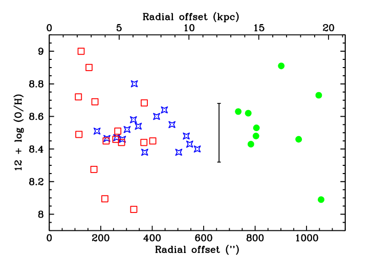
Figure 7: The radial dependence of the oxygen abundance (12 + log(O/H)) from the observed PN modelled by Cloudy (Tab. 8). The points are coded for the three regions as in Fig. 2: F56 by open stars (blue); F42 as open squares (red); F34 by filled circles (green). A representative error bar on the O abundance is shown.

The distribution of [$\alpha$/Fe] v. [Fe] has an important role in determining the enrichment history of a galaxy (e.g. Matteucci & Recchi MatRec (2001)). O, as representing the $\alpha$ elements, is primarily a core collapse SN product released early in star formation activity, whilst Fe, as the chief product of Type Ia SNe, is released over many Gyr. Figure 8 shows the Fe v. Mg b EW plot for the integrated spectra of regions F42 and F56 with several tracks from Thomas et al. (Thomas (2003)) models for selected metallicity and [$\alpha$/Fe] ratio. To be compatible with Harris et al. (Harris00 (2000)), who calibrated their metallicities by assuming that their stars were as old as those in old Galactic globular clusters, then the models must be compared at an age of 15 Gyr. In this case the datapoints for fields F42 and F56 lie close to the tracks of [$\alpha$/Fe] = 0.3, giving an [$\alpha$/Fe] ratio of 0.25, and show metallicities [Z] around -0.6 (there are no tracks at metallicity intermediate between -0.33 and -1.35 in Thomas et al. Thomas (2003)). If, however, the age of the stars were younger (as indicated e.g. by Rejkuba et al. (Rejkuba05 (2005), Rejkuba11 (2011))), the derived metallicities would be about 0.2 higher, giving an average value of -0.4. This would imply an oxygen abundance relative to solar of -0.15, a value that is consistent with the mean O abundance of -0.17 with respect to the solar value (Scott et al. Scott (2009)).

These abundances can also be compared with the MDF from Harris & Harris (Harris02 (2002)) in three fields at 7.6 kpc SW of the centre, at 20 kpc S and 29 kpc S (distances rescaled to 3.8 Mpc). Fig. 9 shows the histogram of all the PN O/H abundances with respect to Solar overplotted against the completeness corrected MDFs in the inner field (7.6 kpc) and two combined outer fields (Table 1 of Harris & Harris Harris02 (2002)). The PN sample covers the range around the inner and outer fields of Harris et al. (Harris02 (2002)). A shift of -0.25 is required to align the peak of the PN O/H distribution with the stellar MDF in the inner field (magenta histogram). However it is strongly apparent that the distribution of (O/H) for the PNe is much narrower than for the stellar metallicity, so matching the distribution peaks may not be a justifiable simplification. Splitting the PN into two samples with positions greater and less than 10 kpc shows a shift in the peak value of (O/H) of $\sim$-0.2 for the inner field and $\sim$-0.3 for the outer field, although the number of PNe with abundances is lower in the outer field (11). For the full PN sample, with an average O abundance of -0.17 compared to Solar, the total metallicity is then -0.4 assuming a mean [$\alpha$/Fe]=0.25. Harris et al. (Harris02 (2002)) find an average metallicity of -0.6 in their outer fields, which becomes -0.4 assuming an age of 8 Gyr; thus taken at face value, assuming the metallicity of the field stars is that of the PN, the age of these stars in NGC 5128 is around 10 Gyr.

Both methods – matching observed spectral indices to stellar population models and comparison with photometrically derived stellar metallicity distributions – provide an average [O/Fe] ratio of 0.25 at a stellar metallicity (viz. [Fe/H]) of around -0.4, and an average age of 8 Gyr. This single value is obviously a simplification for the behaviour in a whole galaxy, but demonstrates that the [O/Fe] v. [Fe/H] value for NGC 5128 is within the range of $\alpha$-enhanced stellar metallicities for early type galaxies (c.f. Thomas et al. Thomas (2003)). The modelling of the colour-magnitude diagram by Rejkuba et al. (Rejkuba11 (2011)) also independently favours $\alpha$-enhanced stellar abundances in NGC 5128.

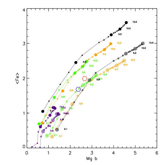
Figure 8: The Lick index $<Fe>$ is plotted against Mg b for the integrated spectra of the two inner fields F42 (red lozenge) and F56 (blue lozenge). Two families of tracks from Thomas et al. (2003) for [$\alpha$/Fe] of 0.3 (open symbols) and 0.0 (filled symbols) are shown for metallicity [Z] of -1.35, -0.33, 0.0 and 0.35 by lines with points. The lower set of four lines have [$\alpha$/Fe] = 0.3, and the upper ones [$\alpha$/Fe]=0. Models with [Z]=0.35 are indicated in black, [Z]=0.0 in orange, [Z]=-0.33 in green and [Z]=-1.35 in magenta. The ages in Gyr along each track are indicated.

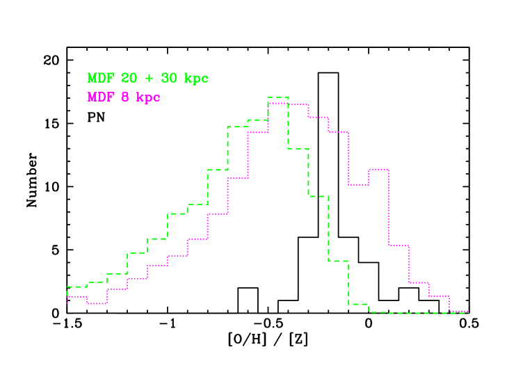
Figure 9: The histogram of the log O/H abundance relative to Solar is plotted for all PN with O/H determined from Cloudy models (Tab. 8) as a continuous line (black). For comparison the stellar metallicity distribution function (MDF) from Harris & Harris (Harris02 (2002)) is plotted in two regions: an inner region (8 kpc) dotted (magenta); a composite of two outer regions at 20 and 30 kpc dashed (green).

However it can be argued that while all the stars are represented in the integrated stellar spectra and photometric surveys, only a subset of these stars become PNe. So, the mean values of the two samples of the PN [O/H] and the stellar [Fe/H] in Fig. 9 are not necessarily strictly comparable. In particular the PNe may derive from a younger population, on average. Only the higher Z stars produce observable PN, while the stellar continuum is comprised of stars of all metallicities. Overall the occurrence of PN is highly delimited relative to all the stars in a galaxy and in addition the PN central star masses also have a very restricted range relative to all white dwarfs. Thus the PNe may only come from a young population; that would explain the tendency toward both higher Z (Fig. 9) and higher central star masses (see Fig. 10). The old stars, which have lower Z on average, fail to produce PNe because their masses are too low.

Chiappini et al. (Chiap (2009)) present a careful comparison of the spectroscopically determined abundances of Milky Way Bulge stars with Bulge planetary nebulae. Their sample of 166 PN in the Bulge with well-determined abundances shows a broad distribution of 12 + log(O/H) from about 8.2 to 8.9, with a mean of 8.57, rather similar to the mean value and range determined here in NGC 5128. However the O/H abundance collated from various spectroscopic studies of Bulge giant stars shows a lower value by $\sim$0.3 dex. Various suggestions are offered by Chiappini et al. (Chiap (2009)) for this discrepancy, but none appears to be conclusive. Comparing O from the Bulge PN with [O/Fe] from the stars, implies [O_PN/Fe_Stars] $\sim$ -0.1. This value is not strictly comparable to that in NGC 5128 since [Fe/H] is derived from photometry; spectroscopy of individual stars in NGC 5128 is ruled out until larger telescopes are available. Taken at face value the difference in [O/Fe] could imply that the formation history of NGC 5128 as a classical giant elliptical, is dissimilar to that of the Bulge; however the discrepancy in O abundances of Bulge PN and giants found by Chiappini et al. (Chiap (2009)) weakens this conclusion as does the large spread in stellar Fe abundances (in both NGC 5128 and the Bulge).

6.4 PN and the star formation history

One of the advantages of running Cloudy models to determine the PN abundances is that the central star luminosities and temperatures are derived. Since the PNe are optically thick, the match to the spectrum effectively provides the temperature and the $m_{5007\AA}$ photometry, combined with the reddening, provides the luminosity. Fig. 10 shows the Log $L$, Log T_eff points for the 40 PNe modelled (Tab. 8). The log $L$ values span a range of a factor 6, but are, not surprizingly, at the high end for PNe central stars, since only the top few magnitudes of the PNLF is explored by these data. No radial trend in the central star luminosities is apparent, paralleling the lack of an O abundance gradient (Fig. 7). A few evolutionary tracks from Vassiliadis & Wood (VasWood (1997)) for higher mass progenitor stars are shown on Fig. 10, although there is currently no information on whether the central stars are on the H or He burning track. For the H burning tracks the bulk of the points match stars with masses above 2 M_⊙.

There are multiple routes in terms of stellar mass, metallicity and mode of turn-off from the AGB (H or He burning track) to reach the same PN luminosity, so relating a given PN in a galaxy to its progenitor star formation episode is non-trivial. Marigo et al. (Marigo (2004)) have modelled effects of stellar populations on the [O III] cut-off of a population of PN, as measured for the PNLF. They find that the peak [O III] luminosity is emitted by stars with initial (main sequence) masses of about 2.5 M_⊙ with a very strong dependence with age. PN from higher mass progenitors, although being intrinsically luminous, evolve very rapidly and so make a minor contribution to the bright end of the PN population. In addition, Ciardullo & Jacoby (Ciardullo99 (1999)) showed that the intrinsically massive and luminous progenitors are prolific dust producers, and therefore self-extinct. Thus the most massive progenitors will generally appear as rare and faint PNe in a galactic sample. Ciardullo et al. (Ciardullo05 (2002)) suggest that the progenitors of the most luminous PNe in galaxies, if they are not formed from stars younger than $\sim$1 Gyr, may occur predominantly in binary systems.

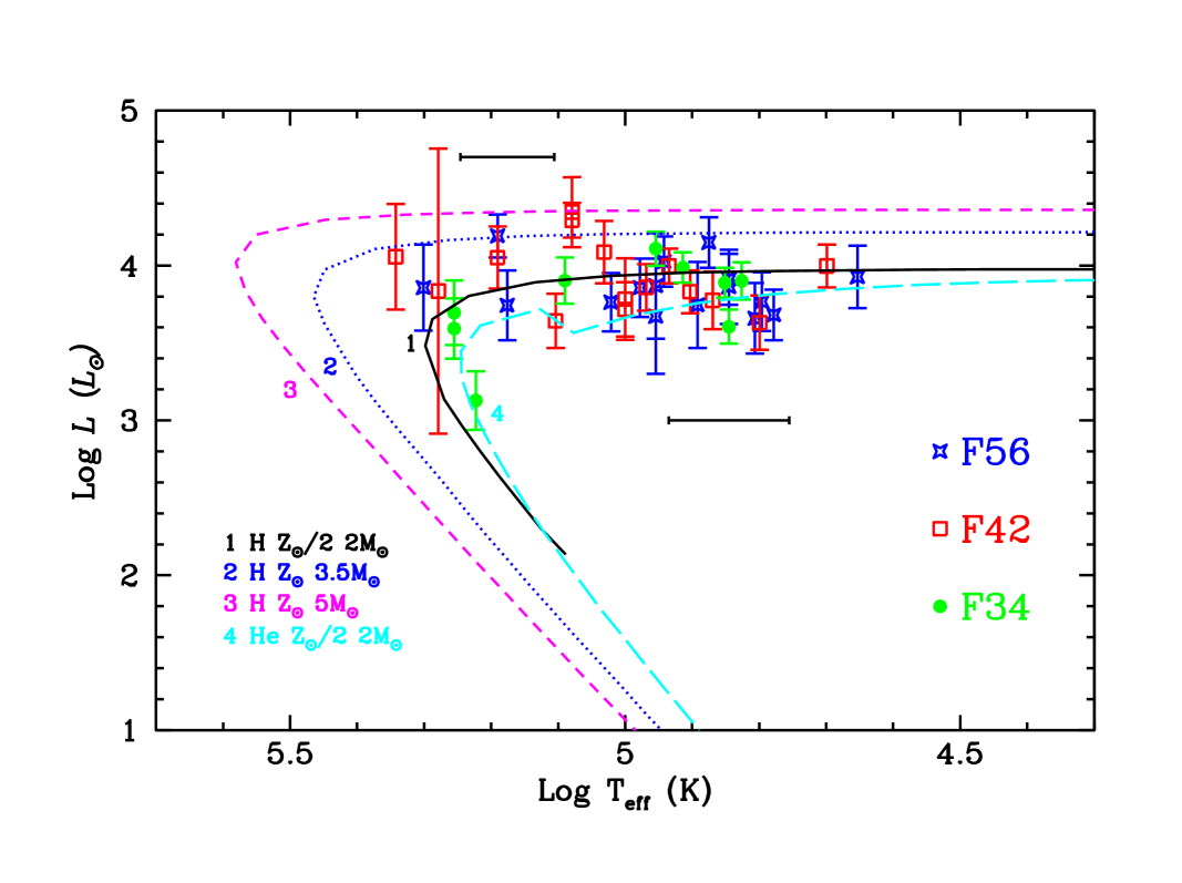
Figure 10: An HR diagram showing the black body log $L$ v. log $T_{eff}$ coordinates of the central stars of the PNe with spectra modelled by Cloudy (Tab. 8) and a selection of low mass H and He burning model tracks from Vassiliadis & Wood (VasWood (1997)). The points are coded (and coloured) for the three regions (F42, F56 and F34) as in Fig. 2. Representative error bars on temperature at higher and lower temperatures are shown; the error bars in $Log\leavevmode\nobreak\ L$ were computed from the errors on dereddened absolute H$\beta$ flux in Tab. References.

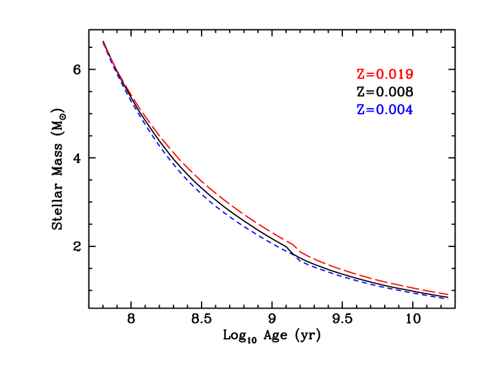
Figure 11: The age at which a star terminates the AGB is shown as a function of the initial main sequence stellar mass for three metallicities of 0.019 (long-dashed line, red), 0.008 (Solar metallicity; continous line, black) and 0.004 (approximately LMC metallicity; short-dashed line, blue). The curves are derived from the stellar evolution tracks of Girardi et al. (Girardi (2000)).

In principle the calibration of PN luminosity v. stellar progenitor mass can be used to identify the age of the starburst giving rise to an observed PN population. If indeed the bulk of the PN observed in this study arise in progenitors of about 2.5 M_⊙, then from the grid of evolutionary tracks of low mass stars of Girardi et al. (Girardi (2000)) one can infer a progenitor age of 0.7 Gyr (see Fig. 11 derived from the Girardi et al. tracks for $[Z/Z_{\odot}]$ 0.0, -0.4 and -0.7 and the stellar age to AGB termination). Such an age would place the PN in a very recent star formation episode. This seems rather unlikely since there is little evidence for an extensive stellar population so young. A young (2-4 Gyr) minority (20-30%) component was inferred from the HST stellar photometric studies of Rejkuba et al. (Rejkuba05 (2005) and Rejkuba11 (2011)), but not with stars younger than 2 Gyr as appears to be required to match the PN. Younger stars are brighter and so should have been well-detected in optical photometry, ruling out their presence in NGC 5128.

If the PNe studied here belong to this minority younger population of age 2-4 Gyr, then the deduced stellar masses, as indicated by the HR diagram of the PN central stars in Fig. 10, are still unexpectedly high. However since these PN belong to the bright end of the luminosity function, there is a selection effect in favour of the more luminous (viz. highest mass) PN progenitor stars. If however the observed PNe arose from an intermediate age population (5-8 Gyr), the progenitor stars would only have a mass of $\sim$1.2 M_⊙ and the discrepancy between their deduced masses and age is more difficult to reconcile with evolutionary tracks of single low mass stars (e.g. Vassiliadis & Wood VasWood (1997)). It would be profitable to study spectroscopically a group of lower luminosity PNe in NGC 5128 to determine if their properties differ from the high $L$ PNe presented in this study.

7 Conclusions

Low resolution spectroscopy of 51 PN in NGC 5128 at a range of galactocentric distance of 2-20 kpc have been obtained with the ESO VLT and FORS1 instrument in multi-slit mode (MOS) in three fields. The PN are drawn from the upper 4 magnitudes of the PN [O III] luminosity function. The emission line spectra have been analysed and lines typical of ionization by hot PN central stars have been measured. The weak [O III]4363Å line was just detected in 20% of the PNe. In order to determine element abundances for a larger fraction of the observed PNe, photoionization modelling was conducted with Cloudy for 40 PN with the highest quality spectra (representing the upper 2 mag. of the PNLF). He, N, O and Ne abundances were determined for all the PNe, and S and Ar for about half of the sample. For the most reliably estimated element, oxygen, no radial gradient is seen and the slope of O/H v. projected radius is identical inside and outside of 10 kpc. The range of [O/H] in the sample spanned -0.66 to +0.31 dex with the mean 12 + log O/H of 8.52 (median 8.48).

The PN O abundances were compared to the stellar abundance measured from Lick indices from the continuum spectroscopy (i.e. along the MOS slitlets not occupied by PN emission) and from resolved star photometry from the literature. If the stars in NGC 5128 have an average age of 8 Gyr, the stellar and PN metallicities agree in the outer parts of NGC 5128 with average values around -0.4 Solar. The deduced masses of the PN central stars implies progenitor masses above 2 M_⊙, favouring their formation from a very young component of the intermediate age stellar population with age ${}^{<}_{\sim}$5 Gyr. This discrepancy between the age of the stellar population and the mass of the PN progenitor stars is in line with other studies of the high mass end of the PN luminosity function.

[x]l l — r r — r r — r r — r r — r r NGC 5128 PN spectra - Observed line fluxes

& F56 #1 F56 #2 F56 #3 F56 #4 F56 #5
5615 5601 5621 5611 5608
($+$297.6,$-$492.5) ($+$284.3,$-$465.9) ($+$287.4,$-$448.7) ($+$298.7,$-$405.0) ($+$268.9, $-$394.1)
Species $\lambda$ (Å) F_Obs $\pm$ F_Obs $\pm$ F_Obs $\pm$ F_Obs $\pm$ F_Obs $\pm$
 [O II] 3727 38 32 43 10 84 20
 [Ne III] 3868 38 14 97 10 55 16 72 19 112 60
 [Ne III] + H$\epsilon$ 3970 29 6
 H$\delta$ 4101 22 8
 H$\gamma$ 4340 36 13 48 9 43 14 31 13 46 48
 [O III] 4363 24 7
 He I 4471 5 3
 He II 4686 37 7
 H$\beta$ 4861 100 0 100 0 100 0 100 0 100 0
 [O III] 4959 298 27 469 32 276 35 332 49 549 64
 [O III] 5007 867 69 1421 93 812 92 965 135 1606 174
 He I 5876 8 4 24 7
 [N II] 6548 44 7 23 6 72 15 74 14
 H$\alpha$ 6562 392 32 396 26 440 51 412 58 420 47
 [N II] 6583 147 14 78 7 284 34 246 35 25 10
 He I 6678 10 6
 [S II] 6716 39 30 21 8
 [S II] 6730 13 7 20 11 11 6
 [Ar III] 7133 17 10 12 4 21 11 59 13 39 34
 [O II] 7325 22 6 104 35 28 12
log F(H$\beta$) -16.37 0.03 -16.06 0.03 -16.50 0.05 -16.39 0.06 -16.59 0.05
m_5007A 24.84 0.09 23.52 0.07 25.22 0.12 24.76 0.15 24.72 0.12


F56 #6 F56 #8 F56 #9 F56 #10 F56 #11
5602 5425 5456 5416 5409
($+$247.7,$-$372.5) ($+$260.2,$-$326.0) ($+$235.0,$-$312.2) ($+$241.5,$-$281.6) ($+$240.2, $-$279.3)
Species $\lambda$ (Å) F_Obs $\pm$ F_Obs $\pm$ F_Obs $\pm$ F_Obs $\pm$ F_Obs $\pm$
 [O II] 3727 42 9 38 10 24 15 29 5
 [Ne III] 3868 75 12 49 13 69 11 96 9
 [Ne III] + H$\epsilon$ 3970 52 8 31 16 53 31 47 23
 H$\delta$ 4101 13 10 27 18 27 7 27 10
 H$\gamma$ 4340 43 7 42 10 43 8 48 9
 [O III] 4363 15 4
 He I 4471
 He II 4686
 H$\beta$ 4861 100 0 100 0 100 0 100 0 100 0
 [O III] 4959 432 35 292 27 263 108 382 29 476 37
 [O III] 5007 1273 100 865 78 794 311 1179 87 1370 103
 He I 5876 14 3 33 8 26 8 11 7
 [N II] 6548 39 5 76 9 29 5 59 11
 H$\alpha$ 6562 468 37 362 33 301 123 388 29 336 77
 [N II] 6583 149 13 233 22 51 36 113 10 161 35
 He I 6678 16 5 18 11
 [S II] 6716 13 4
 [S II] 6730 19 5 12 6 10 3
 [Ar III] 7133 56 9 39 8 51 8 31 7
 [O II] 7325 29 12 46 16 25 19
log F(H$\beta$) -16.08 0.03 -16.13 0.04 -17.37 0.19 -16.14 0.03 -16.12 0.03
m_5007A 23.70 0.09 24.23 0.10 27.43 0.48 23.93 0.08 23.71 0.08


F56 #12a F56 #12b F56 #13b F56 #14 F56 #15
5418 5438 5413 5408 5421
($+$221.9,$-$245.1) ($+$220.2,$-$242.0) ($+$201.5,$-$225.7) ($+$183.5,$-$217.4) ($+$169.1, $-$200.2)
Species $\lambda$ (Å) F_Obs $\pm$ F_Obs $\pm$ F_Obs $\pm$ F_Obs $\pm$ F_Obs $\pm$
 [O II] 3727 77 52 15 11 31 12 28 11
 [Ne III] 3868 129 27 32 11 82 14 84 11 55 12
 [Ne III] + H$\epsilon$ 3970 66 49 27 14 40 13 50 40
 H$\delta$ 4101 15 8 26 9 26 13
 H$\gamma$ 4340 41 13 36 9 40 14 30 11 44 13
 [O III] 4363
 He I 4471
 He II 4686 57 13 13 11
 H$\beta$ 4861 100 0 100 0 100 0 100 0 100 0
 [O III] 4959 684 97 180 20 529 50 445 41 366 45
 [O III] 5007 1956 271 516 51 1540 140 1336 121 1083 128
 He I 5876 20 11 16 8 15 6 23 6
 [N II] 6548 111 19 77 9 67 9 24 8
 H$\alpha$ 6562 420 59 365 36 383 36 382 35 415 49
 [N II] 6583 335 48 266 26 34 7 194 19 63 10
 He I 6678 11 4
 [S II] 6716
 [S II] 6730 12 9 11 5 20 8
 [Ar III] 7133 31 8 32 7 19 8 33 7 21 8
 [O II] 7325 69 20 20 12 58 15
log F(H$\beta$) -16.37 0.06 -16.17 0.04 -16.22 0.04 -16.11 0.04 -16.21 0.05
m_5007A 23.97 0.15 24.91 0.11 23.83 0.10 23.71 0.10 24.19 0.13


F56 #16 F56 #17 F56 #18
5419 5428 5422
($+$139.3,$-$175.8) ($+$146.7,$-$145.7) ($+$107.6,$-$151.4)
Species $\lambda$ (Å) F_Obs $\pm$ F_Obs $\pm$ F_Obs $\pm$
 [O II] 3727 41 16 26 18
 [Ne III] 3868 48 12 26 10 88 21
 [Ne III] + H$\epsilon$ 3970 16 7 18 10 29 15
 H$\delta$ 4101
 H$\gamma$ 4340 37 7 30 8
 [O III] 4363
 He I 4471 20 7
 He II 4686
 H$\beta$ 4861 100 0 100 0 100 0
 [O III] 4959 369 31 275 34 416 74
 [O III] 5007 1063 84 861 101 1315 230
 He I 5876 24 9 30 12 28 13
 [N II] 6548 36 7 102 23
 H$\alpha$ 6562 415 34 356 42 447 79
 [N II] 6583 147 14 323 58
 He I 6678
 [S II] 6716
 [S II] 6730 11 6 30 11
 [Ar III] 7133 24 8
 [O II] 7325
log F(H$\beta$) -16.15 0.03 -16.19 0.05 -16.35 0.08
m_5007A 24.07 0.09 24.41 0.13 24.34 0.19

F42 #1 F42 #2 F42 #3 F42 #4 F42 #6
4504 4502 4527 4506 0530
($-$393.2,$-$84.9) ($-$362.5, $-$71.3) ($-$345.6,$-$126.0) ($-$318.8,$-$79.3) ($-$278.7,$-$34.0)
Species $\lambda$ (Å) F_Obs $\pm$ F_Obs $\pm$ F_Obs $\pm$ F_Obs $\pm$ F_Obs $\pm$
 [O II] 3727 75 37 21 6 44 34
 [Ne III] 3868 61 8 134 17 19 4 28 4 42 7
 [Ne III] + H$\epsilon$ 3970 33 6 51 8 20 3
 H$\delta$ 4101 17 5 19 10 17 4
 H$\gamma$ 4340 37 6 45 29 43 7 42 5 37 7
 [O III] 4363
 He I 4471 5 2
 He II 4686 36 8
 H$\beta$ 4861 100 0 100 0 100 0 100 0 100 0
 [O III] 4959 350 24 625 60 182 13 222 12 289 25
 [O III] 5007 1078 70 1872 177 582 38 663 33 778 64
 He I 5876 28 8 7 2 32 11
 [N II] 6548 65 9
 H$\alpha$ 6562 367 25 462 46 437 29 361 18 349 30
 [N II] 6583 78 7 231 26 203 15 147 8 18 7
 [S II] 6716 20 5 6 2
 [S II] 6730 27 7 12 4 26 11
 [Ar III] 7133 23 6 37 8 30 5
 [O II] 7325 37 6
log F(H$\beta$) -16.56 0.03 -16.78 0.04 -16.62 0.03 -16.43 0.02 -16.62 0.04
m_5007A 25.09 0.07 25.04 0.10 25.89 0.07 25.27 0.05 25.59 0.09


F42 #7 F42 #8 F42 #9 F42 #10 F42 #11
0519 4217 4244 4211 0509
($-$ 253.4,$-$81.8) ($-$229.7, $-$119.5) ($-$209.0,$-$72.3) ($-$179.6,$-$119.8) ($-$165.4,$-$52.4)
Species $\lambda$ (Å) F_Obs $\pm$ F_Obs $\pm$ F_Obs $\pm$ F_Obs $\pm$ F_Obs $\pm$
 [O II] 3727 40 7 12 8 48 4
 [Ne III] 3868 80 9 78 8 66 10 54 5 45 7
 [Ne III] + H$\epsilon$ 3970 36 7 31 7 27 10 18 3
 H$\delta$ 4101 20 6 18 6 22 5 19 5
 H$\gamma$ 4340 40 7 39 7 50 33 44 7 43 10
 [O III] 4363 10 6
 He I 4471
 He II 4686 23 8 20 4
 H$\beta$ 4861 100 0 100 0 100 0 100 0 100 0
 [O III] 4959 512 42 431 31 339 30 271 14 313 26
 [O III] 5007 1522 121 1315 90 1081 90 827 41 973 78
 He I 5876 29 12
 [N II] 6548 58 20 117 24
 H$\alpha$ 6562 410 34 390 28 412 37 447 23 372 33
 [N II] 6583 142 16 161 14 118 14 278 15 226 21
 He I 6678 15 4
 [S II] 6716 22 5
 [S II] 6730 37 7 16 7
 [Ar III] 7133 48 10 29 6 84 25
 [O II] 7325 72 31
log F(H$\beta$) -16.63 0.03 -16.60 0.03 -16.70 0.04 -16.38 0.02 -16.59 0.04
m_5007A 24.87 0.09 24.97 0.08 25.43 0.09 24.90 0.05 25.25 0.09


F42 #12b F42 #13 F42 #14b F42 #15b F42 #16a
4214 4248 4210 4245 4207
($-$135.0,$-$115.2) ($-$115.2, $-$103.1) ($-$99.8,$-$73.0) ($-$68.7,$-$65.2) ($-$48.4,$-$102.4)
Species $\lambda$ (Å) F_Obs $\pm$ F_Obs $\pm$ F_Obs $\pm$ F_Obs $\pm$ F_Obs $\pm$
 [O II] 3727 56 32 50 38 65 14
 [Ne III] 3868 114 15 151 80 160 32 43 9 100 16
 [Ne III] + H$\epsilon$ 3970 64 10 53 32 34 10
 H$\delta$ 4101
 H$\gamma$ 4340 40 12 31 17 44 15
 [O III] 4363 19 8
 He I 4471
 He II 4686 14 12 31 24 58 29
 H$\beta$ 4861 100 0 100 0 100 0 100 0 100 0
 [O III] 4959 569 57 690 356 796 140 270 33 574 74
 [O III] 5007 1747 172 2185 1125 2438 426 872 101 1749 224
 He I 5876
 [N II] 6548 64 16
 H$\alpha$ 6562 504 51 507 263 493 89 432 51 385 52
 [N II] 6583 197 23 246 130 171 36 192 30
 He I 6678
 [S II] 6716
 [S II] 6730 35 10
 [Ar III] 7133
 [O II] 7325 44 19
log F(H$\beta$) -16.73 0.04 -17.10 0.22 -16.88 0.08 -16.64 0.05 -16.65 0.06
m_5007A 24.97 0.11 25.66 0.56 24.99 0.19 25.51 0.13 24.77 0.14


F42 #17 F42 #18
4264 4212
($-$13.9,$-$166.9) ($-$5.9,$-$115.2)
Species $\lambda$ (Å) F_Obs $\pm$ F_Obs $\pm$
 [O II] 3727
 [Ne III] 3868 40 9
 [Ne III] + H$\epsilon$ 3970
 H$\delta$ 4101
 H$\gamma$ 4340 34 8 46 11
 [O III] 4363
 He I 4471
 He II 4686 17 14
 H$\beta$ 4861 100 0 100 0
 [O III] 4959 210 16 553 61
 [O III] 5007 608 42 1616 175
 He I 5876
 [N II] 6548 51 11
 H$\alpha$ 6562 495 36 583 65
 [N II] 6583 191 18 69 16
 He I 6678
 [S II] 6716
 [S II] 6730
 [Ar III] 7133
 [O II] 7325
log F(H$\beta$) -16.61 0.03 -16.65 0.05
m_5007A 25.81 0.07 24.85 0.12

F34 #1 F34 #2 F34 #4 F34 #7 F34 #11
2606 2603 2607 3403 3404
($-$497.0,$-$921.7) ($-$548.8, $-$902.6) ($-$446.9,$-$860.0) ($-$433.1,$-$790.8) ($-$409.1,$-$693.3)
Species $\lambda$ (Å) F_Obs $\pm$ F_Obs $\pm$ F_Obs $\pm$ F_Obs $\pm$ F_Obs $\pm$
 [O II] 3727 64 7 64 7 48 9 55 28 30 11
 [Ne III] 3868 72 5 45 5 49 5 98 6 95 11
 [Ne III] + H$\epsilon$ 3970 25 4 35 6 39 5 28 7
 H$\delta$ 4101 23 4 16 4 24 4 25 5 24 6
 H$\gamma$ 4340 35 3 44 5 46 5 43 6 49 8
 [O III] 4363 9 4 8 2 18 9
 He I 4471 17 4 9 3 18 7
 He II 4686 2 2 8 4 t 48 9
 H$\beta$ 4861 100 0 100 0 100 0 100 0 100 0
 [O III] 4959 404 15 261 13 319 16 535 21 530 45
 [O III] 5007 1214 43 782 37 972 45 1591 62 1574 130
 He I 5876 32 9
 [N II] 6548 33 9
 H$\alpha$ 6562 410 17 528 28 454 24 447 20 421 43
 [N II] 6583 152 9 108 12 151 11 116 9 27 11
 He I 6678 26 6 8 8
 [S II] 6716
 [S II] 6730
 [Ar III] 7133 6 4 39 10 37 7
 [O II] 7325 6 5 33 16

log F(H$\beta$) -16.56 0.02 -16.70 0.03 -16.69 0.03 -16.59 0.03 -16.94 0.05
m_5007A 24.96 0.04 25.78 0.05 25.51 0.05 24.73 0.04 25.62 0.09


F34 #12 F34 #14 F34 #15 F34 #16
3405 3505 3504 3506
($-$424.4,$-$682.1) ($-$458,3,$-$622.8) ($-$490.7,$-$611.0) ($-$434.5,$-$592.1)
Species $\lambda$ (Å) F_Obs $\pm$ F_Obs $\pm$ F_Obs $\pm$ F_Obs $\pm$
 [O II] 3727 48 16 38 4 138 16
 [Ne III] 3868 34 7 66 5 93 9 111 14
 [Ne III] + H$\epsilon$ 3970 30 4 46 9
 H$\delta$ 4101 15 10 20 6
 H$\gamma$ 4340 35 8 47 5 45 6 46 12
 [O III] 4363 7 3 13 5 25 8
 He I 4471 5 3
 He II 4686 45 9 21 15 47 12
 H$\beta$ 4861 100 0 100 0 100 0 100 0
 [O III] 4959 477 45 403 18 455 30 532 50
 [O III] 5007 1426 132 1193 53 1349 87 1647 151
 He I 5876 49 25
 [N II] 6548 88 13
 H$\alpha$ 6562 321 30 380 19 475 34 458 48
 [N II] 6583 21 8 59 7 43 11 418 44
 He I 6678
 [S II] 6716
 [S II] 6730 36 22
 [Ar III] 7133
 [O II] 7325 57 26
log F(H$\beta$) -16.98 0.05 -16.63 0.03 -16.83 0.04 -17.03 0.04
m_5007A 25.84 0.10 25.16 0.05 25.50 0.07 25.81 0.10

[x]l l — r r — r r — r r — r r — r r NGC 5128 PN spectra - extinction corrected line fluxes

& F56 #1 F56 #2 F56 #3 F56 #4 F56 #5
5615 5601 5621 5611 5608
($+$297.6,$-$492.5) ($+$284.3,$-$465.9) ($+$287.4,$-$448.7) ($+$298.7,$-$405.0) ($+$268.9, $-$394.1)
Species $\lambda$ (Å) F_Dered $\pm$ F_Dered $\pm$ F_Dered $\pm$ F_Dered $\pm$ F_Dered $\pm$
 [O II] 3727 50 42 56 13 120 29
 [Ne III] 3868 49 18 124 13 76 22 95 25 150 81
 [Ne III] + H$\epsilon$ 3970 37 8 72 42
 H$\delta$ 4101 27 10
 H$\gamma$ 4340 41 15 58 10 51 17 35 14
 [O III] 4363 28 8
 He I 4471 6 3
 He II 4686 39 8
 H$\beta$ 4861 100 0 100 0 100 0 100 0 100 0
 [O III] 4959 291 26 457 31 268 34 323 47 533 62
 [O III] 5007 836 66 1367 90 772 87 925 129 1536 166
 He I 5876 6 3 18 5
 [N II] 6548 31 5 18 4 46 10 51 10
 H$\alpha$ 6562 282 23 281 19 282 32 282 40 281 32
 [N II] 6583 105 10 55 5 181 21 168 24 17 7
 He I 6678 7 4
 [S II] 6716 24 19 14 5
 [S II] 6730 9 5 13 7 7 4
 [Ar III] 7133 11 6 8 3 12 6 37 8 24 21
 [O II] 7325 14 4 58 20 17 7
c 0.46 0.11 0.48 0.09 0.62 0.16 0.53 0.20 0.56 0.16
log F(H$\beta$) -15.91 0.03 -15.58 0.03 -15.88 0.05 -15.86 0.06 -16.03 0.05
m_5007A 23.73 0.09 22.37 0.07 23.73 0.12 23.49 0.15 23.37 0.12


F56 #6 F56 #8 F56 #9 F56 #10 F56 #11
5602 5425 5456 5416 5409
($+$247.7,$-$372.5) ($+$260.2,$-$326.0) ($+$235.0,$-$312.2) ($+$241.5,$-$281.6) ($+$240.2, $-$279.3)
Species $\lambda$ (Å) F_Dered $\pm$ F_Dered $\pm$ F_Dered $\pm$ F_Dered $\pm$ F_Dered $\pm$
 [O II] 3727 63 13 46 12 31 19 33 6
 [Ne III] 3868 109 17 59 15 87 14 109 11
 [Ne III] + H$\epsilon$ 3970 73 11 36 19 66 38 52 26
 H$\delta$ 4101 18 13 32 20 33 9 30 11
 H$\gamma$ 4340 53 8 47 11 49 10 51 10
 [O III] 4363
 He I 4471
 He II 4686
 H$\beta$ 4861 100 0 100 0 100 0 100 0 100 0
 [O III] 4959 416 34 286 27 262 107 373 29 470 36
 [O III] 5007 1203 94 841 76 789 309 1137 84 1344 101
 He I 5876 10 2 28 7 21 6 10 6
 [N II] 6548 23 3 59 7 21 4 49 10
 H$\alpha$ 6562 281 22 282 26 282 115 281 21 282 64
 [N II] 6583 89 8 181 17 48 34 81 7 135 29
 He I 6678 10 3 14 9
 [S II] 6716 10 3
 [S II] 6730 14 4 10 5 9 2
 [Ar III] 7133 30 5 29 6 34 5 25 6
 [O II] 7325 19 8 33 11 16 12
c 0.71 0.11 0.35 0.13 0.09 0.30 0.45 0.11 0.24 0.32
log F(H$\beta$) -15.37 0.03 -15.78 0.04 -17.37 0.19 -15.69 0.03 -15.88 0.03
m_5007A 21.99 0.09 23.39 0.10 27.44 0.43 23.93 0.08 23.13 0.08


F56 #12a F56 #12b F56 #13b F56 #14 F56 #15
5418 5438 5413 5408 5421
($+$221.9,$-$245.1) ($+$220.2,$-$242.0) ($+$201.5,$-$225.7) ($+$183.5,$-$217.4) ($+$169.1, $-$200.2)
Species $\lambda$ (Å) F_Dered $\pm$ F_Dered $\pm$ F_Dered $\pm$ F_Dered $\pm$ F_Dered $\pm$
 [O II] 3727 106 72 19 14 40 16 36 14
 [Ne III] 3868 172 35 39 13 102 17 105 14 73 16
 [Ne III] + H$\epsilon$ 3970 85 63 32 16 48 15 61 49
 H$\delta$ 4101 18 9 30 11 32 16
 H$\gamma$ 4340 48 15 40 10 46 16 35 11 52 15
 [O III] 4363
 He I 4471
 He II 4686 60 14 14 11
 H$\beta$ 4861 100 0 100 0 100 0 100 0 100 0
 [O III] 4959 665 94 177 19 517 48 435 40 356 44
 [O III] 5007 1872 259 502 49 1488 136 1292 117 1037 123
 He I 5876 15 9 14 7 12 5 19 5
 [N II] 6548 75 13 60 7 50 7 17 6
 H$\alpha$ 6562 283 40 282 28 281 26 283 26 282 34
 [N II] 6583 225 32 205 20 25 5 143 14 42 7
 He I 6678 8 3
 [S II] 6716
 [S II] 6730 8 6 8 4 13 6
 [Ar III] 7133 19 5 23 5 13 6 23 5 13 5
 [O II] 7325 42 13 13 8 37 10
c 0.55 0.20 0.36 0.14 0.43 0.13 0.42 0.13 0.54 0.17
log F(H$\beta$) -15.83 0.06 -15.81 0.04 -15.79 0.04 -15.69 0.04 -15.67 0.05
m_5007A 22.64 0.15 24.04 0.11 22.79 0.10 22.70 0.10 24.19 0.13


F56 #16 F56 #17 F56 #18
5419 5428 5422
($+$139.3,$-$175.8) ($+$146.7,$-$145.7) ($+$107.6,$-$151.4)
Species $\lambda$ (Å) F_Dered $\pm$ F_Dered $\pm$ F_Dered $\pm$
 [O II] 3727 57 21 37 26
 [Ne III] 3868 63 16 31 12 123 30
 [Ne III] + H$\epsilon$ 3970 21 9 21 12 40 20
 H$\delta$ 4101
 H$\gamma$ 4340 43 9 34 9
 [O III] 4363
 He I 4471 22 8
 He II 4686
 H$\beta$ 4861 100 0 100 0 100 0
 [O III] 4959 359 30 270 33 402 72
 [O III] 5007 1018 81 840 98 1249 218
 He I 5876 19 7 26 11 20 10
 [N II] 6548 25 5 64 15
 H$\alpha$ 6562 282 23 283 33 282 50
 [N II] 6583 100 10 203 36
 He I 6678
 [S II] 6716
 [S II] 6730 7 4 18 7
 [Ar III] 7133 15 5
 [O II] 7325
c 0.54 0.11 0.32 0.17 0.64 0.25
log F(H$\beta$) -15.61 0.03 -15.87 0.05 -15.71 0.08
m_5007A 22.77 0.09 23.63 0.13 22.90 0.19

F42 #1 F42 #2 F42 #3 F42 #4 F42 #6
4504 4502 4527 4506 0530
($-$393.2,$-$84.9) ($-$362.5, $-$71.3) ($-$345.6,$-$126.0) ($-$318.8,$-$79.3) ($-$278.7,$-$34.0)
Species $\lambda$ (Å) F_Dered $\pm$ F_Dered $\pm$ F_Dered $\pm$ F_Dered $\pm$ F_Dered $\pm$
 [O II] 3727 111 56 26 7 52 40
 [Ne III] 3868 74 10 192 24 26 5 34 5 50 9
 [Ne III] + H$\epsilon$ 3970 40 8 71 11 24 4
 H$\delta$ 4101 20 6 24 12 20 4
 H$\gamma$ 4340 41 7 55 36 52 8 47 6 41 7
 [O III] 4363
 He I 4471 5 3
 He II 4686 39 9
 H$\beta$ 4861 100 0 100 0 100 0 100 0 100 0
 [O III] 4959 343 23 602 58 176 13 218 12 284 25
 [O III] 5007 1046 68 1772 168 554 36 645 32 760 63
 He I 5876 24 6 6 2 28 10
 [N II] 6548 42 6
 H$\alpha$ 6562 281 19 281 28 282 19 281 14 281 24
 [N II] 6583 60 6 140 16 131 10 114 6 15 6
 [S II] 6716 15 4 5 2
 [S II] 6730 20 6 9 3 21 8
 [Ar III] 7133 16 4 22 5 22 4
 [O II] 7325 28 5
c 0.37 0.09 0.69 0.14 0.61 0.09 0.35 0.07 0.30 0.12
log F(H$\beta$) -16.19 0.03 -16.09 0.04 -16.01 0.03 -16.08 0.02 -16.32 0.04
m_5007A 24.19 0.07 23.37 0.10 24.41 0.07 24.43 0.05 24.86 0.09


F42 #7 F42 #8 F42 #9 F42 #10 F42 #11
0519 4217 4244 4211 0509
($-$ 253.4,$-$81.8) ($-$229.7, $-$119.5) ($-$209.0,$-$72.3) ($-$179.6,$-$119.8) ($-$165.4,$-$52.4)
Species $\lambda$ (Å) F_Dered $\pm$ F_Dered $\pm$ F_Dered $\pm$ F_Dered $\pm$ F_Dered $\pm$
 [O II] 3727 52 9 16 11 69 6
 [Ne III] 3868 105 12 99 10 87 13 76 6 55 9
 [Ne III] + H$\epsilon$ 3970 46 9 38 9 34 13 24 5
 H$\delta$ 4101 25 7 22 7 28 7 22 6
 H$\gamma$ 4340 47 8 44 8 59 38 52 9 48 11
 [O III] 4363 12 7
 He I 4471
 He II 4686 24 8 21 5
 H$\beta$ 4861 100 0 100 0 100 0 100 0 100 0
 [O III] 4959 498 41 421 30 330 29 262 14 306 26
 [O III] 5007 1460 116 1268 87 1036 86 786 39 944 76
 He I 5876 23 9
 [N II] 6548 37 13 89 18
 H$\alpha$ 6562 282 23 283 21 282 25 282 15 281 25
 [N II] 6583 97 11 116 10 80 10 175 10 170 16
 He I 6678 9 3
 [S II] 6716 14 3
 [S II] 6730 23 4 12 5
 [Ar III] 7133 30 7 17 3 59 17
 [O II] 7325 44 19
c 0.52 0.12 0.45 0.10 0.53 0.13 0.64 0.07 0.39 0.12
log F(H$\beta$) -16.11 0.03 -16.15 0.03 -16.17 0.04 -15.74 0.02 -16.20 0.04
m_5007A 23.61 0.09 23.88 0.08 24.15 0.09 23.36 0.05 24.31 0.09


F42 #12b F42 #13 F42 #14b F42 #15b F42 #16
4214 4248 4210 4245 4207
($-$135.0,$-$115.2) ($-$115.2, $-$103.1) ($-$99.8,$-$73.0) ($-$68.7,$-$65.2) ($-$48.4,$-$102.4)
Species $\lambda$ (Å) F_Dered $\pm$ F_Dered $\pm$ F_Dered $\pm$ F_Dered $\pm$ F_Dered $\pm$
 [O II] 3727 91 52 78 60 83 18
 [Ne III] 3868 174 22 230 122 240 48 59 13 125 20
 [Ne III] + H$\epsilon$ 3970 94 14 78 46 42 12
 H$\delta$ 4101
 H$\gamma$ 4340 51 15 37 20 50 17
 [O III] 4363 21 9
 He I 4471
 He II 4686 15 13 33 26 62 32
 H$\beta$ 4861 100 0 100 0 100 0 100 0 100 0
 [O III] 4959 545 55 660 341 763 135 261 32 561 73
 [O III] 5007 1637 161 2046 1053 2290 401 831 96 1688 216
 He I 5876
 [N II] 6548 46 12
 H$\alpha$ 6562 282 29 282 146 281 51 281 33 281 38
 [N II] 6583 110 13 136 72 97 21 139 22
 He I 6678
 [S II] 6716
 [S II] 6730 22 6
 [Ar III] 7133
 [O II] 7325 29 12
c 0.81 0.14 0.82 0.72 0.78 0.25 0.60 0.17 0.44 0.19
log F(H$\beta$) -15.92 0.04 -16.28 0.22 -16.10 0.08 -16.04 0.05 -16.21 0.06
m_5007A 23.01 0.11 23.69 0.56 23.11 0.19 24.06 0.13 23.71 0.14


F42 #17 F42 #18
4264 4212
($-$13.9,$-$166.9) ($-$5.9,$-$115.2)
Species $\lambda$ (Å) F_Dered $\pm$ F_Dered $\pm$
 [O II] 3727
 [Ne III] 3868 67 14
 [Ne III] + H$\epsilon$ 3970
 H$\delta$ 4101
 H$\gamma$ 4340 43 10 61 14
 [O III] 4363
 He I 4471
 He II 4686 19 15
 H$\beta$ 4861 100 0 100 0
 [O III] 4959 201 16 524 58
 [O III] 5007 571 39 1490 161
 He I 5876
 [N II] 6548 29 6
 H$\alpha$ 6562 281 20 283 32
 [N II] 6583 108 10 33 8
 He I 6678
 [S II] 6716
 [S II] 6730
 [Ar III] 7133
 [O II] 7325
c 0.79 0.10 1.01 0.16
log F(H$\beta$) -15.82 0.03 -15.64 0.05
m_5007A 23.91 0.07 22.41 0.12

F34 #1 F34 #2 F34 #4 F34 #7 F34 #11
2606 2603 2607 3403 3404
($-$497.0,$-$921.7) ($-$548.8, $-$902.6) ($-$446.9,$-$860.0) ($-$433.1,$-$790.8) ($-$409.1,$-$693.3)
Species $\lambda$ (Å) F_Dered $\pm$ F_Dered $\pm$ F_Dered $\pm$ F_Dered $\pm$ F_Dered $\pm$
 [O II] 3727 86 9 106 12 71 13 80 41 41 15
 [Ne III] 3868 93 6 71 7 70 7 137 8 127 15
 [Ne III] + H$\epsilon$ 3970 31 5 48 8 53 7 36 9
 H$\delta$ 4101 28 5 23 6 31 6 33 7 31 7
 H$\gamma$ 4340 41 4 56 7 56 7 52 7 57 10
 [O III] 4363 11 5 9 3 21 11
 He I 4471 20 5 10 3 20 8
 He II 4686 2 2 8 4 t 51 10
 H$\beta$ 4861 100 0 100 0 100 0 100 0 100 0
 [O III] 4959 393 15 249 13 307 15 517 21 514 43
 [O III] 5007 1164 41 729 34 922 43 1512 59 1505 124
 He I 5876 21 6
 [N II] 6548 23 6
 H$\alpha$ 6562 283 12 281 15 281 15 282 12 282 28
 [N II] 6583 104 6 57 6 93 7 73 6 18 8
 He I 6678 13 3 5 5
 [S II] 6716
 [S II] 6730
 [Ar III] 7133 4 3 21 5 21 4
 [O II] 7325 4 3 17 9
c 0.52 0.06 0.88 0.07 0.67 0.08 0.64 0.06 0.56 0.14
log F(H$\beta$) -16.04 0.02 -15.82 0.03 -16.02 0.03 -15.95 0.03 -16.38 0.05
m_5007A 23.70 0.04 23.66 0.05 23.89 0.05 23.18 0.04 24.27 0.09


F34 #12 F34 #14 F34 #15 F34 #16
3405 3505 3504 3506
($-$424.4,$-$682.1) ($-$458,3,$-$622.8) ($-$490.7,$-$611.0) ($-$434.5,$-$592.1)
Species $\lambda$ (Å) F_Dered $\pm$ F_Dered $\pm$ F_Dered $\pm$ F_Dered $\pm$
 [O II] 3727 53 17 48 6 203 24
 [Ne III] 3868 37 7 82 6 135 14 157 19
 [Ne III] + H$\epsilon$ 3970 36 5 64 13
 H$\delta$ 4101 18 13 26 8
 H$\gamma$ 4340 37 8 53 6 55 8 55 15
 [O III] 4363 8 3 16 6 30 10
 He I 4471 5 3
 He II 4686 46 9 23 16 50 13
 H$\beta$ 4861 100 0 100 0 100 0 100 0
 [O III] 4959 473 45 394 18 438 29 513 48
 [O III] 5007 1405 130 1153 51 1274 82 1560 143
 He I 5876 45 23
 [N II] 6548 54 8
 H$\alpha$ 6562 282 26 281 14 282 20 281 29
 [N II] 6583 18 7 43 6 25 6 255 27
 He I 6678
 [S II] 6716
 [S II] 6730 21 13
 [Ar III] 7133
 [O II] 7325 48 22
c 0.18 0.13 0.42 0.07 0.73 0.10 0.68 0.15
log F(H$\beta$) -16.81 0.05 -16.22 0.03 -16.10 0.04 -16.36 0.04
m_5007A 25.41 0.10 24.15 0.05 23.73 0.07 24.17 0.10