Spatio-temporal stochastic resonance induces patterns in wetland vegetation dynamics
Abstract
Water availability is a major environmental driver affecting riparian and wetland vegetation. The interaction between water table fluctuations and vegetation in a stochastic environment contributes to the complexity of the dynamics of these ecosystems. We investigate the possible emergence of spatial patterns induced by spatio-temporal stochastic resonance in a simple model of groundwater-dependent ecosystems. These spatio-temporal dynamics are driven by the combined effect of three components: (i) an additive white Gaussian noise, accounting for external random disturbances such as fires or fluctuations in rain water availability, (ii) a weak periodic modulation in time, describing hydrological drivers such as seasonal fluctuations of water table depth, and (iii) a spatial coupling term, which takes into account the ability of vegetation to spread and colonize other parts of the landscape. A suitable cooperation between these three terms is able to give rise to ordered structures which show spatial and temporal coherence, and are statistically steady in time.
keywords:
spatio-temporal stochastic resonance , spatial pattern formation , wetland vegetation dynamics1 Introduction
Random fluctuations can play an important role in determining the composition and structure of ecosystems [3, 15]. Fire occurrences [9], fluctuations in rain water availability [27, 17, 11], soil heterogeneity [33], and temperature oscillations [32], are some of the examples of fluctuating environmental drivers. Evaluating ecosystem response to environmental fluctuations is crucial, among other things, to the management and restoration of plant communities [55, 37], the understanding of their ability to sustain biodiversity [26, 23, 10], and to predict causes of possible shifts in vegetation composition [35, 6, 55].
The effects of noise on dynamical systems has been studied in a number of stochastic models proposed in recent years [42, 14]. Noise is typically associated with a ”destroying effect”, as a driver of disorganized fluctuations around the stable states of the underlying deterministic dynamics. However, a number of studies have demonstrated the existence of a ”constructive effect” of noise: ordered spatial structures (i.e. patterns) can emerge in some spatio-temporal dynamical systems as a result of noisy fluctuations (see, for example, [36, 43, 50, 29, 45]). An increase in noise intensity can produce in these systems a counterintuitive, more regular and organized, behaviour both in time and in space.
For example, the cooperation of a random external driver with an external periodic forcing is able to induce ordered transitions between different states of a dynamical system. Known as stochastic resonance (see, among others, [13, 20, 51]), this phenomenon may occur when a bistable system is disturbed by an external random forcing in the presence of a weak periodic fluctuation in time. Bistable system exhibit a bistable potential with two minima separated by a potential barrier. The periodic forcing causes fluctuations in the height of the potential barrier, without ever causing a transition between the two states. It is the external random forcing - if strong enough - that is able to drive the system from a stable state to the other; these transitions are more likely to occur when the height of the potential barrier is lowest, which depends on the phase of the periodic fluctuations. A suitable synchronization between the frequency of the random transitions (which is related to the noise intensity) and the frequency of the periodic forcing induces a resonance-like effect that generates regular transitions between the two stable states [53, 31].
Even though a number of studies have recognized the bistable character of some ecosystems [39, 5, 56, 37] and the ability of random fluctuations to induce new dynamical behaviours that do not exist in the underlying deterministic dynamics [2, 8], applications of stochastic resonance theories to eco-hydrology have started to appear only recently (see, for instance, [4, 46, 34, 47]).
In this paper we study the basic mechanisms for the occurrence of spatio-temporal stochastic resonance in a simple model describing the dynamics of riparian or wetland vegetation dynamics. The temporal deterministic dynamics of the model have been proposed by Ridolfi et al. [37] to investigate the emergence of bistability from the interactions between phreatophyte vegetation and shallow phreatic aquifers in wetland ecosystems. The combined effect of external noise and periodic oscillations on these bistable dynamics has been shown to be able to induce stochastic resonance in the time domain [4].
We investigate the possible emergence of spatio-temporal stochastic resonance when a diffusive spatial coupling term is introduced in the presence of random and periodic forcings. The addition of a spatial diffusive mechanism accounts for the vegetation ability to encroach across the landscape. The other assumptions are physically based, due to the presence of environmental disturbances (e.g. occurrence of fires, rainfall fluctuations) acting on the system, and a number of periodic hydrological drivers (e.g., seasonal oscillations of the water table). In particular, a significant connection exists between water table fluctuations and vegetation dynamics. The water level variation appears to be an independent and important vegetation gradient, as the responses of species to the range of water level fluctuations seem to reflect their tolerance to disturbances [18]. Changes in species composition and distribution, as well as in vegetation structure, have been related to various factors, mainly the vegetation topographical position with respect to the water table, frequency and duration of inundation [24]. It has been observed that, under the periodic declining groundwater availability, vegetation patches tend to show a regular spatial behaviour [16]. Moreover, in dune systems, the occurrence of regular patterns of heath patches has been associated, among other things, to the different groundwater discharge [25].
The relevant question here is whether the phenomenon of stochastic resonance - resulting from the combined effect of noise and a weak temporal oscillation - can interact with a spatial diffusive term to generate vegetation ordered spatial structures.
2 Modeling framework
We consider the dynamics of plant biomass, , and its interplay with the phreatic aquifer [37]. We first recall some important aspects of the temporal deterministic dynamics, and then present the characteristics of the spatio-temporal stochastic system.
2.1 Deterministic model
Changes in vegetation biomass are the result of a growth-death process that can be expressed as (e.g., [28, 48]),
| (1) |
where is the dimensionless biomass, normalized by a (high) fixed reference value, is the dimensionless time (where controls the temporal response of the system and is time), and is the dimensionless ecosystem carrying capacity, that is the maximum amount of vegetation sustainable with the available resources.
The interaction between phreatophyte vegetation, i.e. plants relying on the phreatic aquifer, and the average depth of the local water table is widely recognized as one of the key aspects affecting wetland ecosystems dynamics [30, 41, 7, 37]. For example, the water table decreases in the presence of phreatophyte species because of the lower recharge rates due to rainfall interception and plant transpiration [54, 1, 38, 12], and also because vegetation taproots directly extract water from the aquifer [19]. The depth, , of the water table is adimensionalized with respect to water table depth in the absence of vegetation, , and can be expressed as a linear function of plant biomass, ,
| (2) |
where is the dimensionless sensitivity of the water table to the presence of vegetation. is positive because plants typically tend to increase the depth of the water table. The water table depth, , in turn affects the dynamics of wetland vegetation. If the water table is too shallow (waterlogging), vegetation can suffer, due to an insufficient aeration of the root zone and a decreased rate of seedling establishment [41]. If the water table is too deep, water is out of reach of taproots and vegetation can suffer as well. These effects are taken into account by a quadratic dependence of the carrying capacity, , on the water table depth, ,
| (3) |
where regulates the sensitivity of carrying capacity to changes in water table depth, and are the adimensional thresholds of vegetation tolerance to shallow and deep water tables, respectively.
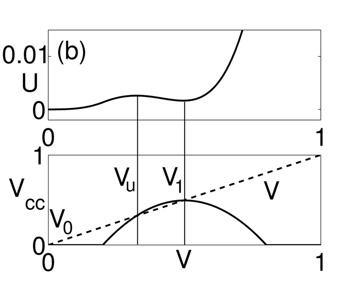
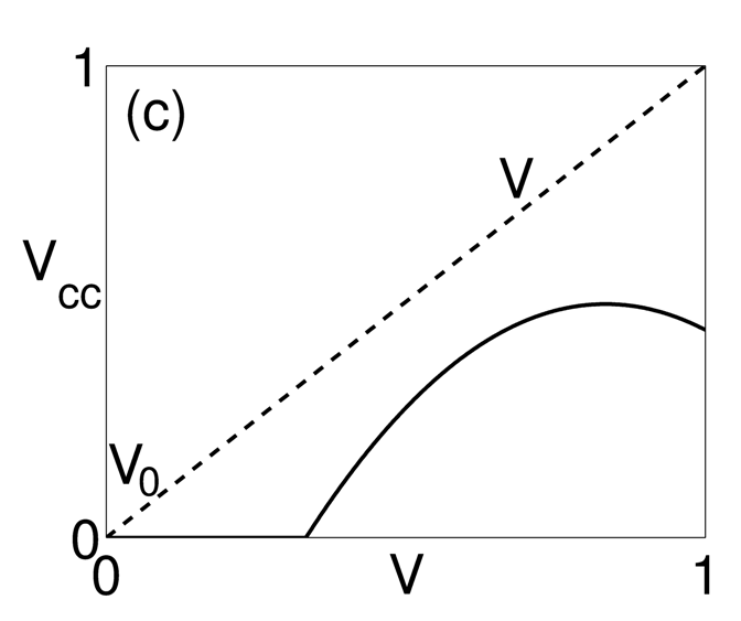
A positive feedback may exist between vegetation establishment and water table dynamics, whereby phreatophytes favor their own survival by increasing the water table depth and enhancing root aeration [54, 7]. The presence of positive feedback mechanisms suggests the possible existence of multiple stable states [37]. This fact is confirmed by some experimental evidence suggesting that two alternative equilibrium states may exist in wetland vegetation dynamics [41, 6, 55, 44]. Equilibrium states can be found by setting Eq. (1) equal to zero. is always an equilibrium state, therefore the existence of multiple equilibrium states depends on the existence of real, nonnull roots of the equation . These solutions can be found by substituting Eq. (2) in Eq. (3), and then searching for intersections between and (see Fig. 1). Ridolfi et al. [37] showed three possible cases:
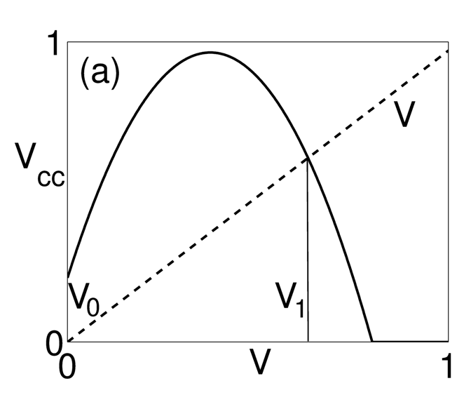
(a) (Fig. 1a). The water table depth in the absence of vegetation, , is always greater than the minimum depth required for vegetation establishment. is an unstable state and only one stable state exists, . Ecosystem dynamics always tend the vegetated state, , regardless the initial conditions.
(b) (Fig. 1b) and vegetation is able to keep the water table below the maximum elevation acceptable for plants (e.g. ), three equilibrium states are found. Two of these states, and are stable, while the other one, , is unstable. If grows above , then the system tends to the vegetated state. Otherwise, it evolves towards the unvegetated state and remains here blocked. Note that the two stable states correspond to the minima of the double-well potential, U(V), with , while the unstable solution, corresponds to a maximum or ”potential barrier”.
(c) (Fig. 1c) and vegetation is not able to reduce the water table elevation below the minimum level suitable for plant survival (e.g. ). In this case the only possible stable state is the unvegetated condition, .
2.2 Spatio-temporal stochastic model
We now focus on the case (b) described above, with two stable states (vegetated and unvegetated) emerging from the deterministic dynamics. We introduce in these dynamics three new terms: (i) a periodic temporally oscillating term, accounting for seasonal or interannual fluctuations of the water table depth, , [40, 57]; (ii) a random forcing term, representing the effect of random environmental drivers (e.g., fires or climate fluctuations); (iii) a spatial coupling term, modeling the diffusive spread of vegetation.
Eq. (1) now reads,
| (4) |
where is the strength of the spatial coupling, is the Laplace operator, is a white (in time and space) Gaussian noise with zero mean, intensity , and correlation , being the Dirac delta function. The temporal oscillation is directly inserted into Eq. (4), through the dependence of on the water table depth, Eq. (2), which can be now expressed as
| (5) |
where and are the nondimensional amplitude and the dimensional frequency of the seasonal oscillations, respectively. is the oscillation period (for example 1 year). Notice that these seasonal fluctuations of the water table are crucial to the emergence of the dynamical behaviors (i.e., spatiotemporal stochastic resonance) presented and discussed in the following sections. Therefore, Eq. (3) now reads
| (6) |
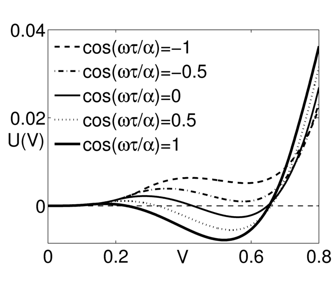
We consider the case of relatively weak seasonal oscillations in a way that the potential, , still has two minima corresponding to two stable states. Fig. 2 shows the potential, , of the temporal deterministic model (1), but with the water table depth, , modulated as in (5). The potential always maintains two minima throughout its periodic oscillation. Thus, even though there are phases in the modulation of the periodic forcing in which the height of the potential barrier is strongly reduced (hence, the probability of occurrence of a state transition is enhanced), deterministic transitions between the two wells of the potential are not allowed.
The choice of an additive white (Gaussian) noise to represent external drivers acting on vegetation dynamics in the time domain is motivated by the fact that the temporal scales of the random driver are typically much shorter than the characteristic temporal scales over which the temporal vegetation dynamics evolve (e.g. the relaxation time to a stable state). Moreover we used a white noise also in space to show how spatial coherence is not imposed by the spatial correlation of these external driver but emerges as an effect of spatio-temporal stochastic resonance. Therefore, this kind of noise is typically adopted in stochastic modeling [42].
The Laplacian, , in Eq. (4) is a simple operator which is widely used to represent the spatial effects of the diffusion mechanisms in vegetation dynamics [3, 22, 52]. This operator accounts for spatial interactions between a point of the domain and its nearest neighbors, and is therefore considered as a short-range spatial coupling.
3 Results
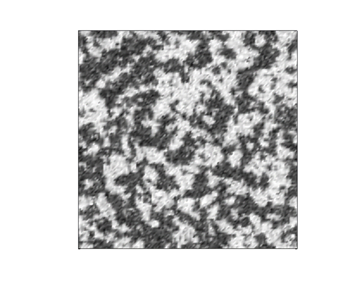
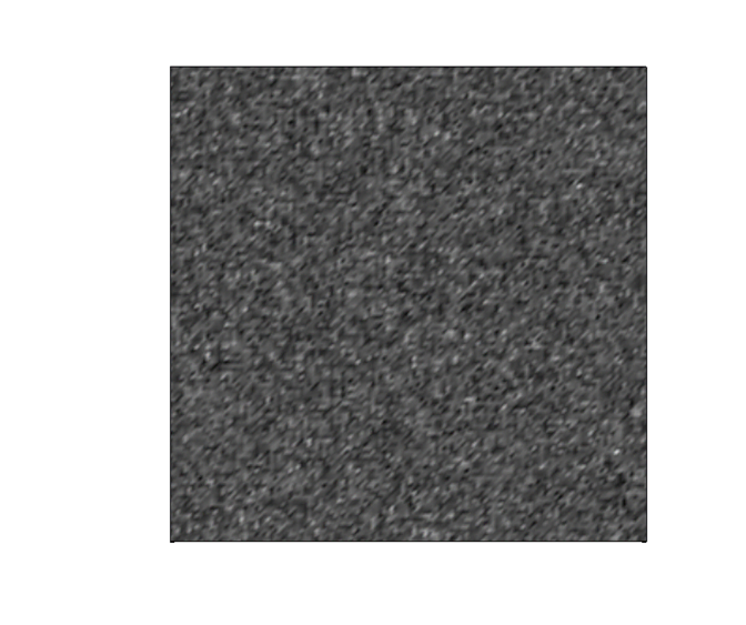
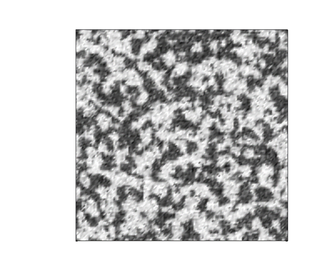
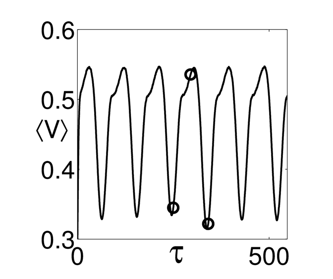
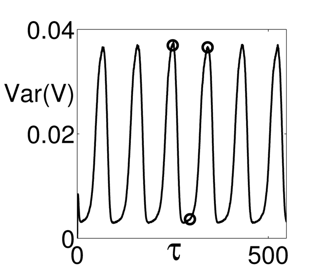

The model (4) is numerically solved for different parameter sets to directly investigate the associated spatio-temporal vegetation dynamics. Periodic boundary conditions are adopted, while, in the absence of other indications, the initial conditions used in the simulations are uniformly distributed random numbers in the range [0.29, 0.31]. We also use the mean field analysis, a mathematical framework that provides the steady-state probability distribution of [36, 49, 50]. Details about the numerical scheme and the mean-field analysis are reported in A.
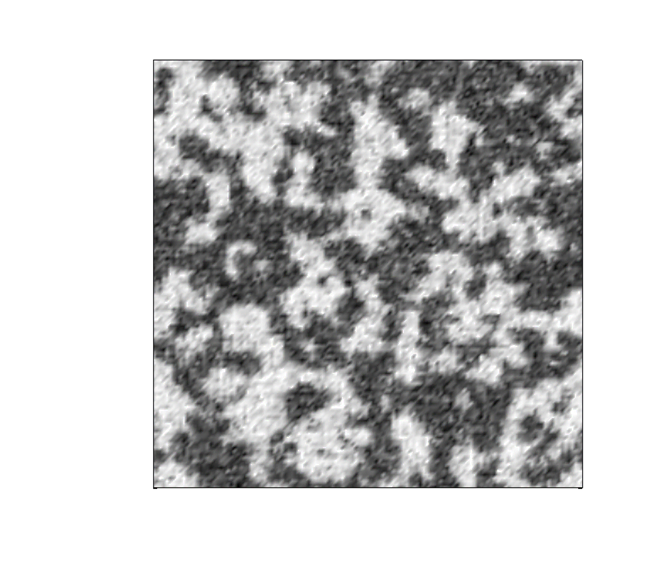
Fig. 3 shows numerical results for and (other parameter values are reported in the caption of the figure). Black and white tones are used for the highest () and lowest () values of , respectively. Well defined patterns periodically emerge (e.g., at and ) and disappear () in the course of periodic fluctuations of . In this case the non-dimensional period is . Pattern occurrence corresponds to temporal minima of mean vegetation biomass and to maxima of biomass variance, while homogeneous vegetated states correspond to maxima of mean biomass and minima of the variance of vegetation biomass (see circles in Fig. 3). Here and in the following discussion, we call ”homogeneous” a state in which the system exhibits negligible spatial heterogeneity with respect to the patterned state.
The spatio-temporal dynamics continuously oscillate between two differently vegetated states. In this example patterns appear during the transition between these two states, when the system approaches the least vegetated stable state, and disappear when the most vegetated state is reached. The interaction of noise with periodic water table oscillations and spatial diffusion gives rise to spatial ordered structures which are statistically steady and periodically appear/disappear in time with the same period, , as the fluctuations in . These periodic state transitions, and the associated formation and disappearance of spatial patterns are the evidence of spatio-temporal stochastic resonance, with noise-induced shifts between the two minima of the potential, . Although the system tends to oscillate between two stable states, these states are not always reached. Indeed, temporal oscillations have to be sufficiently long to permit the system to visit both states. Here, for example, the temporal period, days, is too short and does not allow the system to reach the unvegetated state. Conversely, with a longer period, , the system is able to attain both the vegetated and the unvegetated states (see Section 3.3).
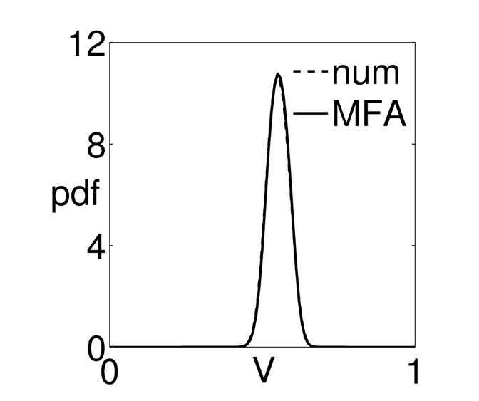
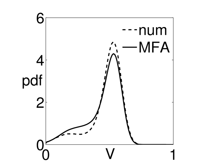
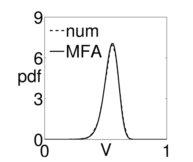
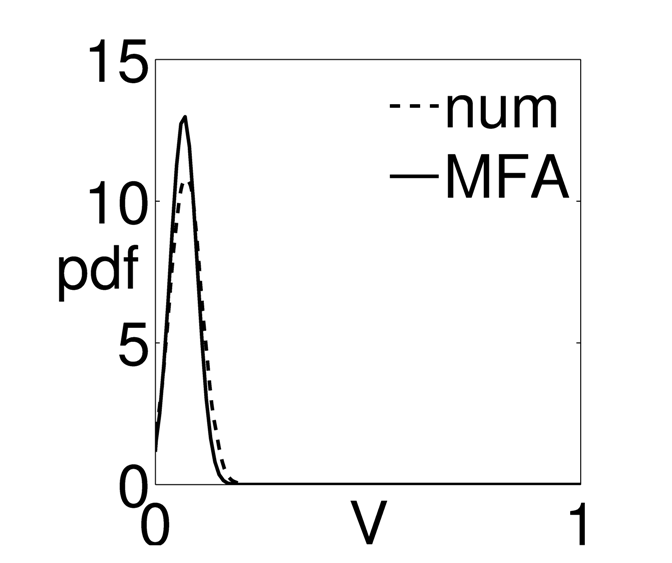
In Fig. 3 numerical and analytical evaluations of the pdf of the vegetation field are reported. Here and in the following discussion, the numerical approximation of the pdf (dashed curves) is obtained using simulated fields in the temporal range , which encompasses several temporal oscillation periods (here, ). Details on the analytical approximation of the pdf (solid curves) are discussed in A. The agreement between numerical and analytical evaluations of the pdf is quite good in showing a weak bimodality.
3.1 Role of and
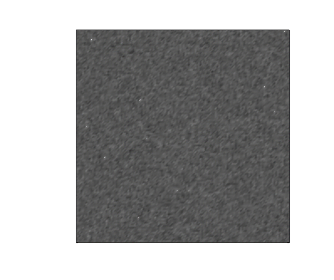

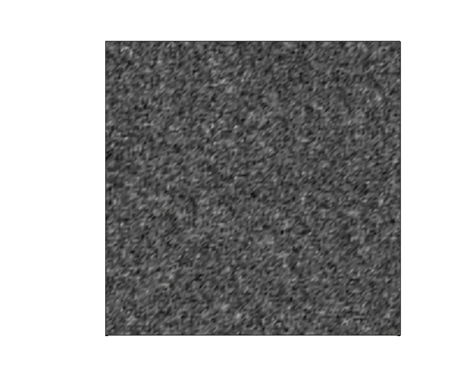
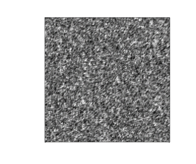
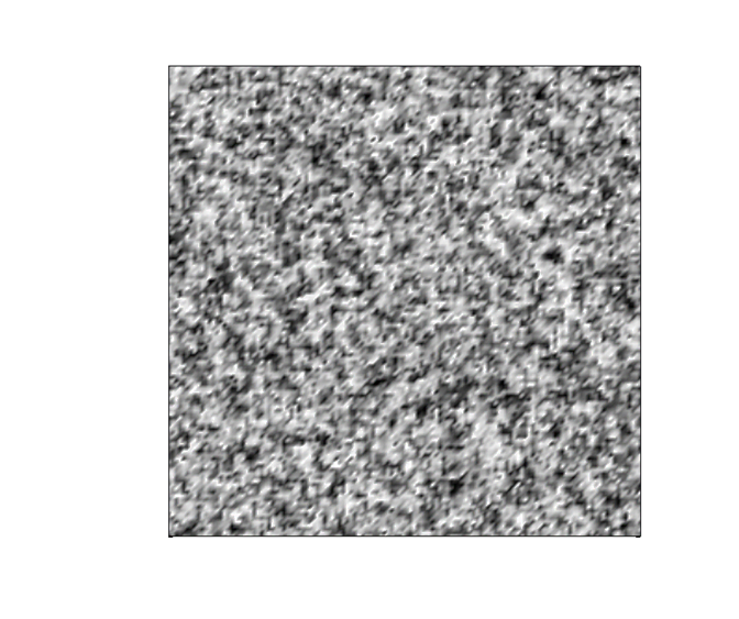
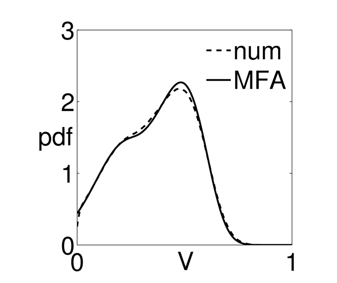
We now consider changes in the spatial coupling strength, (), with a fixed noise intensity (e.g. ). As increases, the least vegetated state moves closer the most vegetated one. As a consequence, for higher values, the system becomes more homogeneous (the biomass variance oscillates around lower values and the amplitude of these fluctuations becomes smaller). By increasing from to , spatially coherent patterns appear. If is further increased, the diffusive effect is so strong that the field is almost homogeneous, and the system experiences a blocking effect induced by diffusion.
Different noise levels () with a fixed spatial coupling () are then considered. If the noise intensity is weak () with respect to the spatial coupling strength, , the biomass density tends to be homogeneous in time and space. On the other hand, if the noise level is too strong (), the system experiences random oscillations between more vegetated and less vegetated states. However, in this case noise has a ”destroying” effect in that it destroys any spatial and temporal coherence and no ordered states emerge. An intermediate noise value () allows for the emergence of temporal fluctuations and the formation of periodic spatial patterns. The existence of an intermediate noise level which, in cooperation with a weak temporal oscillation, is able to regularly move the system between different states is the most typical feature of the stochastic resonance phenomenon [53, 13]. In Fig. 4, we show the configuration of the system in correspondence to local minima ( for , for , for ) and maxima ( for , for , for ) of biomass variance (left and central columns, respectively) for the three values of noise intensity.
In general, temporal local maxima (minima) of biomass variance correspond to minima (maxima) of biomass mean only when the system is able to exhibit ordered spatial structures (see Fig. 3). In all the other cases – i.e. with homogeneous (Fig. 4, top) or disturbed (Fig. 4, bottom) spatial distributions – there is not such a synchronization between maxima (minima) of biomass variance and minima (maxima) of biomass mean.
Also in these cases, there is a very good agreement between the mean-field steady-state pdfs (solid curves) and the pdfs numerically calculated (dashed curves) using simulated fields in the temporal range . This result is especially interesting because this mean-field analysis accounts for the modulation of the dynamics in time (see A), an approach that has never been reported before.
From the results here presented, we can conclude that there is an optimal region in the plane, in which spatial patterns emerge. This region corresponds to a noise intensity, , of order , and a spatial coupling strength, , of order of magnitude .
3.2 Influence of initial conditions


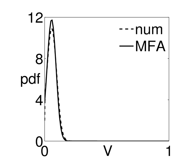


In the previous sections the initial conditions were generated as random numbers uniformly distributed in the interval [0.29, 0.31]. If noise is sufficiently strong with respect to the spatial coupling strength, , results similar to those shown in figures 3, and 4 (middle and bottom), are obtained with different initial conditions. Conversely, if the noise intensity, , is small with respect to , the system tends to an homogeneous steady state, which depends on the initial conditions. In other words, a sufficiently high noise intensity with respect to the spatial coupling strength allows the system to continuously oscillate in time between the two minima of the potential, regardless the initial conditions. On the contrary, if noise is small with respect to the spatial coupling strength, the system remains trapped into the minimum of the potential which is closer to the initial conditions.
An example is shown in Fig. 5 where, for and , different initial conditions, uniformly distributed in the interval [0, 0.02] or [0.29, 0.31], lead to an unvegetated (top) or a vegetated (bottom) state, respectively. When the initial conditions are in the interval [0, 0.02], the system is initially close to the minimum of the potential (). The noise intensity is so weak with respect to the spatial coupling strength, , that it is not able to move the system away from this stable state; therefore the system remains blocked into the unvegetated stable state.
3.3 Different periodicity of the temporal modulation
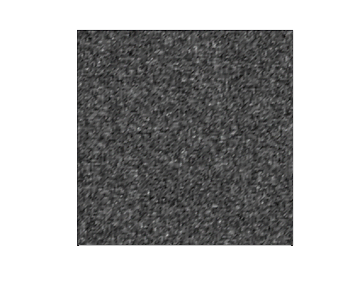
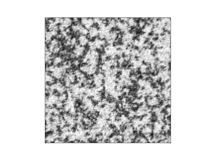
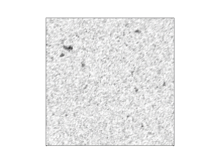
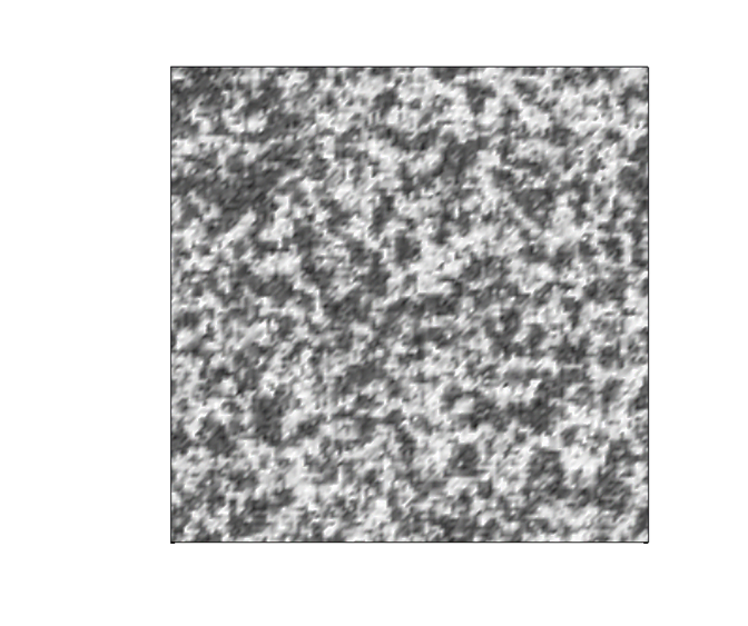
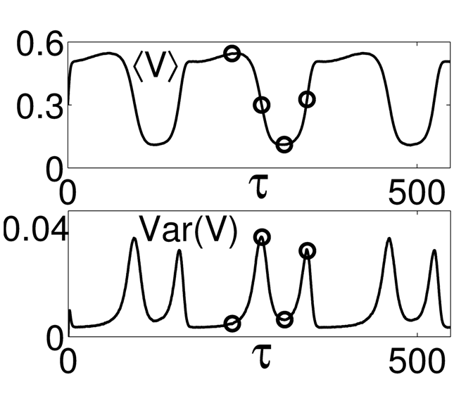
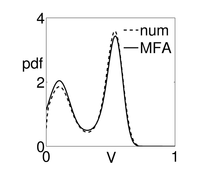
We then evaluate the effect of a different temporal periodicity in the modulation term, , by taking days, while all the other parameters remain the same as in Fig. 3. Patterns periodically emerge ( and ) and disappear ( and ). Their occurrence corresponds to temporal local maxima of the vegetation variance, while homogeneous vegetated and unvegetated stable states correspond to maxima and minima of the vegetation mean, respectively (see circles in Fig. 6). A longer period, , allows the system to explore the whole range of values of . This fact is confirmed by a non-negligible bimodality of both analytical and numerical pdfs, whose peaks correspond to the two alternatively visited stable states. During these state transitions, patterns appear. Although the temporal modulation establishes the frequency of pattern appearance, the mechanism of pattern formation is always present and does not depend on the specific temporal periodicity imposed into the system.
3.4 Non-simultaneous presence of random and periodic forcings

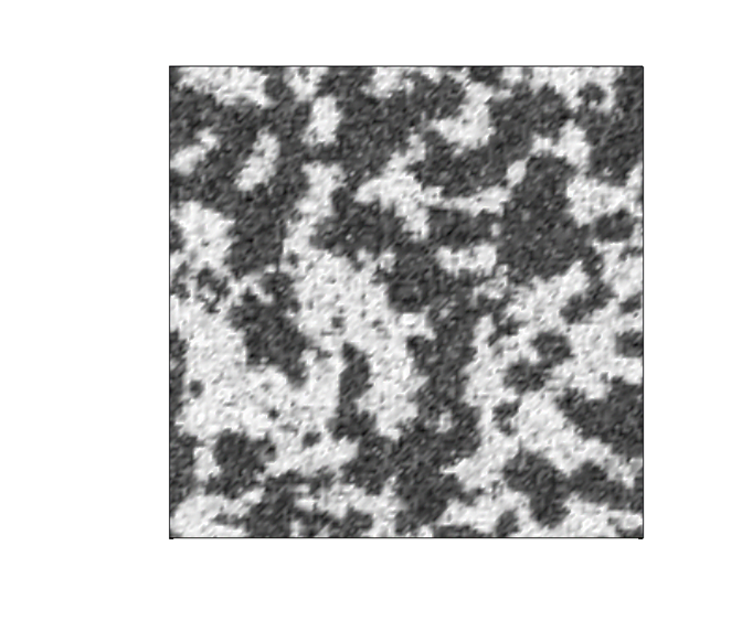
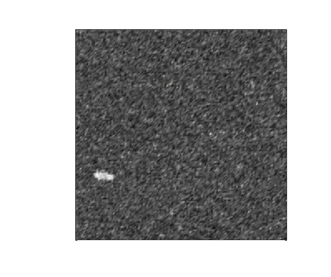


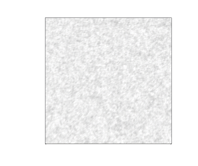
We now consider the case in which noise and temporal modulation do not occur at the same time. As noted, as the noise level, , decreases the spatial distribution of plant biomass becomes more homogeneous. A similar behavior is expected to occur for . The homogeneous state depends on the initial conditions: if the system is initially in the interval [0, 0.02] it homogeneously decays to zero, while for initial conditions in the interval [0.29, 0.31] it reaches the homogeneous vegetated stable state and weakly oscillates in time around it.
When noise is present with no modulation (), state transitions may occur. If the noise is weak with respect to the strength of the spatial coupling, , the homogeneous steady state attained by the system depends on the initial conditions. If the noise is strong enough with respect to , the system tends to the homogeneous vegetated state regardless of the initial conditions. Patterns can emerge only as transient features before the system approaches the homogeneous steady state. An example is shown in Fig. 7 where , the initial conditions are in the interval [0, 0.02], (top) and (bottom). For , while passing from an unvegetated initial condition () to a homogeneous vegetated steady state (), the system exhibits some transient patterns (), which fade out in the long run. Instead, for the noise is weak with respect to and therefore the system is blocked into the low vegetated state without even showing transient patterns.
4 Discussion and conclusions
In the system investigated in this paper the occurrence of spatio-temporal stochastic resonance can be thought of as the result of the combined effect of three components: a white (in time and space) Gaussian noise, a weak periodic modulation in time, and a suitable spatial coupling term. In the absence of modulation, the noise - if strong enough with respect to the spatial coupling - can lead the system towards the vegetated state, regardless of the initial conditions. However, if the noise is weak with respect to , the system will approach one of the two (vegetated or unvegetated) stable states, depending on the initial conditions. With no modulation, patterns can only occur in an initial transient because, once the stable state is reached, the system is locked in a homogeneous state. On the other hand, in the absence of noise the temporal modulation is not able to promote a state transition, because the system reaches one of the two stable states – depending on initial conditions – and weakly oscillates around it. The spatial coupling term is able to induce spatial coherence without itself enhancing state transitions. In other words, noise is the driver able to induce state transitions, while the periodic forcing and the spatial coupling are able to induce temporal and spatial coherence, respectively. Only a suitable cooperation between these three mechanisms can lead to the interesting ordered scenarios analyzed in Section 3. Thus, random and periodic forcings have to be simultaneously present along with a suitable spatial coupling to induce the formation of statistically steady ordered structures with spatial and temporal coherence.
Changes in the periodicity, , of the weak temporal modulation strongly affect vegetation dynamics. In this case, if is of the order of six months or one year, coherent spatial structures periodically appear during transitions between vegetated and unvegetated states. These dynamics could represent the emergence and disappearance of an herbaceous species, which typically have a growth/life period comparable to the driving seasonal oscillations of the water table. Conversely, the emergence of patterns in model simulations with longer periods may represent the formation of ordered structures in the distribution of tree species, which grow over longer time scales.
Beside this interpretation based on a single species, spatial patterns result from the simultaneous existence of two different species, whose growth/life periods are comparable to but not synchronized with one anther (i.e. when species 1 is at maximum density, species 2 is at minimum density). The first species is dominant at a certain time (almost homogeneous field, see, for example, left top panel of Fig. 6), but it tends to disappear, while the density of other increases. The simultaneous presence of both may give rise to ordered spatial structures (spatial pattern occurrence, see middle top panel of Fig. 6). At some point, the second species temporarily dominates the plant community composition (almost homogeneous field, see right top panel of Fig. 6), but it will then start to decay, while the first species grows back and new patterns emerge (see left bottom panel of Fig. 6).
Appendix A Numerical and analytical methods
The typical numerical approach used to solve stochastic partial differential equations is based on a discretization of the continuous spatial domain using a regular Cartesian lattice with spacing . A two-dimensional square lattice with 128x128 sites and is here adopted. The original equation (4) is then transformed into a system of coupled stochastic ordinary differential equations with a finite difference scheme,
| (7) |
where and are the values of and at site , respectively, is the set of the four nearest neighbors of the site . Numerical simulations are carried out with the Heun’s predictor-corrector scheme [50, 42], with a temporal step . Notice how this method does not prevent the emergence of a spurious spatial correlation associated with the discrete representation of the dynamics in a 2D lattice [21]. In our analyses the simulations were repeated with grids of different sizes and the same qualitative patterns and dynamical behaviors were observed to emerge regardless of the resolution used in the discrete representation of the domain.
A qualitative representation of (stochastic) spatio-temporal dynamics can be obtained through the mean-field method. Its fundamental assumption is that the mean of the values of in all the neighboring cells can be approximated by the spatio-temporal mean of the field, namely . Therefore, eq. (7) becomes
| (8) |
The classic mean-field analysis allows one to evaluate if a phase transition occurs. The existence of multiple solutions, , of the self-consistency equation
| (9) |
indicates the presence of a non-equilibrium phase transition. In Eq. (9) is the temporal modulation and is the conditional probability with respect to at steady state. We recall that the occurrence of non-equilibrium phase transition is neither a necessary nor a sufficient condition for noise-induced pattern formation [36, 43]. In fact, non-equilibrium phase transitions imply that noise is able to change the value of the order parameter, but not that ordered geometrical structures necessarily emerge.
Here, the dynamics exhibit also a temporal modulation, , which has to be adequately accounted for while applying the mean-field method. To evaluate the steady state pdf of the biomass vegetation, , and at the same time to deal with the temporal modulation , we propose to solve the self-consistency condition (9) for all the values of . In this way the conditional probability, , is obtained. The steady-state probability is then computed through the convolution product between the conditional probability, , and the probability, , of the temporal modulation, .
Depending on , and values, one or three solutions of the self-consistency equation (9) can be found. If the solution of (9) is unique, then it is considered as the steady state solution. If three solutions are obtained, we can assume that the lowest one corresponds to the least vegetated stable state (), the highest one to the most vegetated stable state (), while the one in the middle to the unstable state (). If the temporal period, , is sufficiently long (e.g. or days) to allow the dynamics to fully develop and periodically visit the two stable states, all the three solutions are taken into account as steady state solutions. If, instead, the period is much shorter (e.g. days), the dynamics are able to completely reach only one of the two stable states, while the other one remains unexplored. As a result, the system oscillates in time and fully captures only one stable state, while the other one is not approached. Only the explored stable state and the unstable state are considered as steady state solutions.
Once solutions, , of (9) are determined, their conditional probabilities, , are computed as
| (10) |
and
| (11) |
where is the potential of the temporal deterministic model (1) with water table depth, , modulated as in (5). Since the pdf, , of the cosine function, , is
| (12) |
the probability can be evaluated through the convolution integral
| (13) |
If, for a given value of , two or more conditional probabilities, , exist, they are summed together and then weighted with the same probability (defined by ) to compute the probability . The probability is in the end normalized so that .
References
- Borg et al. [1988] Borg, H., Stoneman, G. L., Ward, C. G., 1988. The effect of logging and regeneration on groundwater, streamflow and stream salinity in the southern forest of western australia. J. Hydrol. 99, 253–270.
- Borgogno et al. [2007] Borgogno, F., D’Odorico, P., Laio, F., L., R., 2007. Effect of rainfall interannual variability on the stability and resilience of dryland plant ecosystems. Water Resour. Res. 43, W06411.
- Borgogno et al. [2009] Borgogno, F., D’Odorico, P., Laio, F., Ridolfi, L., 2009. Mathematical models of vegetation pattern formation in ecohydrology. Rev. Geophys. 47, RG1005.
- Borgogno et al. [2011] Borgogno, F., D’Odorico, P., Laio, F., Ridolfi, L., 2011. Stochastic resonance and coherence in groundwater-dependent plant ecosystems. Submitted to J. Theor. Biol.
- Brovkin et al. [1998] Brovkin, V., Claussen, M., Petoukhov, V., Ganopolski, A., 1998. On the stability of the atmosphere-vegetation system in the sahara/sahel region. J. Geophys. Res. 103, 31613–31624.
- Chambers and Linnerooth [2001] Chambers, J. C., Linnerooth, A. R., 2001. Restoring riparian meadows currently dominated by artemisia using alternative state concepts - the establishment component. Appl. Veg. Sci. 4, 157–166.
- Chang [2002] Chang, M., 2002. Forest hydrology: An introduction to water and forests. CRC Press, Boca Raton, FL.
- D’Odorico et al. [2005] D’Odorico, P., Laio, F., L., R., 2005. Noise-induced stability in dryland plant ecosystems. Proc. Natnl. Acad. Sci. USA 102, 10819.
- D’Odorico et al. [2007] D’Odorico, P., Laio, F., Porporato, A., Ridolfi, L., Barbier, N., 2007. Noise-induced vegetation patterns in fire-prone savannas. J. Geophys. Res. - Biogeosci. 112, G02021.
- D’Odorico et al. [2008] D’Odorico, P., Laio, F., Ridolfi, L., Lerdau, M., 2008. Biodiversity enhancement induced by environmental noise. J. Theor. Biol. 255, 332–337.
- D’Odorico and Porporato [2006] D’Odorico, P., Porporato, A., 2006. Dryland ecohydrology. Springer-Verlag, New York.
- Dubé et al. [1995] Dubé, S., P., P. A., Rothwell, R. L., 1995. Watering up after clear-cutting on forested wetlands of the st. lawrence lowland. Water Resour. Res. 31, 1741–1750.
- Gammaitoni et al. [1998] Gammaitoni, L., Hänggi, P., Jung, P., Marchesoni, F., 1998. Stochastic resonance. Rev. Mod. Phys. 70, 223–287.
- García-Ojalvo and Sancho [1999] García-Ojalvo, J., Sancho, J. M., 1999. Noise in Spatially Extended Systems. Springer-Verlag, New York.
- Holling [1973] Holling, C. S., 1973. Resilience and stability of ecological systems. Annu. Rev. Ecol. Syst. 4, 1–23.
- Kong et al. [2009] Kong, W., Sun, O. J., Xu, W., Chen, Y., 2009. Changes in vegetation and landscape patterns with altered river water-flow in arid west china. J. Arid Environ. 73, 306–313.
- Laio et al. [2001] Laio, F., Porporato, A., Ridolfi, L., Rodriguez-Iturbe, I., 2001. Plants in water-controlled ecosystems: active role in hydrologic processes and response to water stress - ii. probabilistic soil moisture dynamics. Adv. Water Resour. 24, 707–723.
- Laitinen et al. [2008] Laitinen, J., Rehell, S., Oksanen, J., 2008. Community and species responses to water level fluctuations with reference to soil layers in different habitats of mid-boreal mire complexes. Plant Ecol. 194, 17–36.
- Le Maitre et al. [1999] Le Maitre, D. C., Scott, D. F., Colvin, C., 1999. A review of information on interactions between vegetation and groundwater. Water SA 25, 137–152.
- Lindner et al. [1995] Lindner, J. F., Meadows, B. K., Ditto, W. L., 1995. Array enhanced stochastic resonance and spatiotemporal synchronization. Phys. Rev. Lett. 75, 3–6.
- Lythe and Habib [2001] Lythe, G., Habib, S., 2001. Stochastic PDEs: convergence to the continuum? Comput. Phys. Commun. 142, 29–35.
- Manor and Shnerb [2008] Manor, A., Shnerb, N. M., 2008. Facilitation, competition, and vegetation patchiness: From scale free distribution to patterns. J. Theor. Biol. 253, 838–842.
- Mitsch and Gosselink [2000] Mitsch, W. J., Gosselink, J. G., 2000. Wetlands. Wiley, New York.
- Moreno-Casasola and Vazquez [1999] Moreno-Casasola, P., Vazquez, G., 1999. The relationship between vegetation dynamics and water table in tropical dune slacks. J. Veg. Sci. 10, 515–524.
- Munoz-Reinoso and de Castro [2005] Munoz-Reinoso, J. C., de Castro, F., 2005. Application of a statistical water-table model reveals connections between dunes and vegetation at donana. J. Arid Environ. 60, 663–679.
- Naiman and Decamps [1997] Naiman, R., Decamps, H., 1997. The ecology of interfaces: Riparian zones. Annu. Rev. Ecol. Syst. 28, 621–658.
- Noy-Meir [1973] Noy-Meir, I., 1973. Desert ecosystems: Environment and producers. Annu. Rev. Ecol. Syst. 4, 25–51.
- Noy-Meir [1975] Noy-Meir, I., 1975. Stability of grazing systems: An application of predator-prey graphs. J. Ecol. 63, 459–481.
- Parrondo et al. [1996] Parrondo, J. M. R., van den Broeck, C., Buceta, J., de la Rubia, F. J., 1996. Noise-induced spatial patterns. Physica A 224, 153–161.
- Peck and Williamson [1987] Peck, A. J., Williamson, D. R., 1987. Effects of forest clearings on groundwater. J. Hydrol. 94, 47–65.
- Perc [2008] Perc, M., 2008. Stochastic resonance on weakly paced scale-free networks. Phys. Rev. E 78, 036105.
- Polyak [1996] Polyak, I., 1996. Observed versus simulated second-moment climate statistics in gcm verification problems. J. Atmos. Sci. 53, 677–694.
- Puigdefabregas et al. [1999] Puigdefabregas, J., Sole, A., Gutierrez, L., del Barrio, G., Boer, M., 1999. Scales and processes of water and sediment redistribution in drylands: results from the rambla honda field site in southeast spain. Earth-Science Rev. 48, 39–70.
- Rao et al. [2009] Rao, F., Wang, W. M., Li, Z. Q., 2009. Spatiotemporal complexity of a predator-prey system with the effect of noise and external forcing. Chaos Soliton. Fract. 41, 1634–1644.
- Ridolfi et al. [2007] Ridolfi, L., D’Odorico, P., Laio, F., 2007. Vegetation dynamics induced by phreatophyte-aquifer interactions. J. Theor. Biol. 248, 301–310.
- Ridolfi et al. [2011] Ridolfi, L., D’Odorico, P., Laio, F., 2011. Noise-Induced Phenomena in the Environmental Sciences. Cambridge University Press, New York.
- Ridolfi et al. [2006] Ridolfi, L., P., D., Laio, F., 2006. Effect of vegetation-water table feedbacks on the stability and resilience of plant ecosystems. Water Resour. Res. 42, W01201.
- Riekerk [1989] Riekerk, H., 1989. Influence of silvicultural practices on the hydrology of pine flatwoods in florida. Water Resour. Res. 25, 713–719.
- Rietkerk and van de Koppel [1997] Rietkerk, M., van de Koppel, J., 1997. Alternate stable states and threshold effects in semi-arid grazing systems. Oikos 79, 69–76.
- Rosenberry and Winter [1997] Rosenberry, D. O., Winter, T. C., 1997. Dynamics of water-table fluctuations in an upland between two prairie-pothole wetlands in north dakota. J. Hydrol. 191, 1–4.
- Roy et al. [2000] Roy, V., Ruel, J. C., Plamondon, A. P., 2000. Establishment, growth and survival of natural regeneration after clearcutting and drainage on forested wetlands. For. Ecol. Manag. 129, 253–267.
- Sagues et al. [2007] Sagues, F., Sancho, J. M., García-Ojalvo, J., 2007. Spatio-temporal order out of noise. Rev. Mod. Phys. 79, 829–882.
- Scarsoglio et al. [2011] Scarsoglio, S., Laio, F., D’Odorico, P., Ridolfi, L., 2011. Spatial pattern formation induced by gaussian white noise. Math. Biosci. 229, 174–184.
- Schroder et al. [2005] Schroder, A., Persson, L., de Roos, A. M., 2005. Direct experimental evidence for alternative stable states: A review. Oikos 110, 3–19.
- Sieber et al. [2007] Sieber, M., Malchow, H., Schimansky-Geier, L., 2007. Constructive effects of environmental noise in an excitable prey-predator plankton system with infected prey. Ecol. Complex. 4, 223–233.
- Spagnolo et al. [2004] Spagnolo, B., Valenti, D., Fiasconaro, A., 2004. Noise in ecosystems: A short review. Math. Biosci. Eng. 1, 185–211.
- Sun et al. [2010] Sun, G. Q., Jin, Z., Liu, Q. X., Li, B. L., 2010. Rich dynamics in a predator-prey model with both noise and periodic force. Biosystems 100, 14–22.
- Tsoularis and Wallace [2011] Tsoularis, A., Wallace, J., 2011. Analysis of logistic growth models. Math. Biosci. 179, 21–55.
- van den Broeck et al. [1994] van den Broeck, C., Parrondo, J. M. R., Toral, R., 1994. Noise-induced nonequilibrium phase transition. Phys. Rev. Lett. 73, 3395–3398.
- van den Broeck et al. [1997] van den Broeck, C., Parrondo, J. M. R., Toral, R., Kawai, R., 1997. Nonequilibrium phase transitions induced by multiplicative noise. Phys. Rev. E 55, 4084.
- Vilar and Rubi [1997] Vilar, J. M. G., Rubi, 1997. Spatiotemporal stochastic resonance in the swift-hohenberg equation. Phys. Rev. Lett. 78, 2886–2889.
- von Hardenberg et al. [2010] von Hardenberg, J., Kletter, A. Y., Yizhaq, H., Nathan, J., Meron, E., 2010. Periodic versus scale-free patterns in dryland vegetation. Proc. R. Soc. B 277, 1771–1776.
- Wellens et al. [2004] Wellens, T., Shatokhin, V., Buchleitner, A., 2004. Stochastic resonance. Rep. Progr. Phys. 67, 45–105.
- Wilde et al. [1953] Wilde, S. A., Steinbrenner, E. C., Pierce, R. S., Dosen, R. C., Pronin, D. T., 1953. Influence of forest cover on the state of the ground water table. Soil Sci. Soc. Am. J. 17, 65–67.
- Wright and Chambers [2002] Wright, J. M., Chambers, J. C., 2002. Restoring riparian meadows currently dominated by artemisa using alternative state concepts - above-ground vegetation response. Appl. Veg. Sci. 5, 237–246.
- Zeng et al. [2004] Zeng, X. D., Shen, S. S. P., Zeng, X. B., Dickinson, R. E., 2004. Multiple equilibrium states and the abrupt transitions in a dynamical system of soil water interacting with vegetation. Geophys. Res. Lett. 31, L05501.
- Zhang and Schilling [2006] Zhang, Y. K., Schilling, K. E., 2006. Effects of land cover on water table, soil moisture, evapotranspiration, and groundwater recharge: A field observation and analysis. J. Hydrol. 319, 328–338.