Electrostatic-field-induced dynamics in an ultrathin quantum well

Abstract

We consider the time evolution of a particle subjected to both a uniform electrostatic field $F$ and a one-dimensional delta-function potential well. We derive the propagator ${\mathcal{K}}_{F}(x,t|x^{\prime},0)$ of this system, directly leading to the wavefunction $\psi_{F}(x,t)$, in which its essential ingredient ${\mathcal{K}}_{F}(0,t|0,0)$, accounting for the ionization-recombination in the bound-continuum transition, is exactly expressed in terms of the multiple hypergeometric functions $F(z_{1},z_{2},\cdots,z_{n})$. And then we obtain the ingredient ${\mathcal{K}}_{F}(0,t|0,0)$ in an appropriate approximation scheme, expressed in terms of the generalized hypergeometric functions ${}_{p}F_{q}(z)$ being much more transparent to physically interpret and much more accessible in their numerical evaluation than the functions $F(z_{1},z_{2},\cdots,z_{n})$.

I Introduction

The ionization of atoms in an external electric field is, as well-known, one of the oldest subjects in quantum physics. As a simple example of the ionization, hydrogen-like atoms in a uniform electrostatic field have been extensively considered (see, e.g., YAM77 ; Raz03 ). Here the background potential caused by the field decreases without limit in one direction, and the electron initially in the bound state will eventually tunnel through the “barrier” created by the field, so leading to ionization of the atom. The tunneling rate for an ensemble of many independent electrons has been calculated based on the exponential decay law following from the statistical assumption that the tunneling rate is proportional to the number of available atoms.

On the other hand, big experimental advances in the field of nano-scale physics have highly enlarged a need for a detailed understanding of the (time-dependent) tunneling process of individual electrons subjected to an external field. In fact, the nano-scale devices have been designed and fabricated, examples of which are molecular switches JOA86 and resonant tunnel junctions JON89 , etc. However, in exploring the time evolution of the electron tunneling process leading to ionization, we have a considerable mathematical difficulty that there are no exactly solvable models for a transition from a bound state to the continuum. Further, even obtaining the numerical solution, with high accuracy, to this problem cannot be considered an easy task either, especially in the strong-field limit where a highly oscillatory behavior is found in the time evolution of the bound-continuum transition.

The system under investigation in this paper is a particle subjected to an attractive one-dimensional delta-function potential, $-V_{0}\,\delta(x)$. We intend to study analytically the time evolution of the particle when a uniform electrostatic field $F$ is applied. The delta-function potential well (not in an external field) has a single bound state. This aspect may rather simplify the analytical study of the ionization. However, no exact solution $\psi_{F}(x,t)$ to the time-dependent Schrödinger equation of this problem has been found in closed form (in terms of the actual calculability to any sufficient degree of precision), even for such a simple form of external field.

In fact, this model of the field-induced time-dependent ionization has already been studied by some people. It was first discussed by Geltman GEL77 . Later on, several different approaches to obtaining the time-dependent wavefunction $\psi_{F}(x,t)$ have been carried out LUD87 ; ELK88 ; SUS90 ; KLE94 ; ENG95 ; ROK00 . One of the approaches mainly adopted so far is to turn the relevant time-dependent Schrödinger equation into the Lippmann-Schwinger integral equation [cf. Eqs. (4) and (7)]. This integral equation is, however, highly non-trivial to solve analytically and so has been focused mostly upon its numerical solvability. In ELK88 ; ELB87 by Elberfeld and Kleber, interestingly enough, the time-dependent ionization probability has been investigated in the strong-field limit based on the numerical analysis of the integral equation. They also demonstrated numerically that the ionization probability obtained from the simple exponential decay law may be considered a fairly good approximation on the average to the exact result in the strong-field limit although this approximation, by construction, cannot account for the short-time ripples, observed in the exact one, which result from the ionization-recombination process in the bound-continuum transition ELK88 ; REI85 .

The goal of this paper lies in a systematic derivation of the propagator ${\mathcal{K}}_{F}(x,t|x^{\prime},0)$ of the system, directly leading to $\psi_{F}(x,t)=\int_{-\infty}^{\infty}dx^{\prime}\,{\mathcal{K}}_{F}(x,t|x^{\prime},0)\,\psi_{0}(x^{\prime})$. As our central finding, its essential constituent part ${\mathcal{K}}_{F}(0,t|0,0)$, accounting for the ionization-recombination, is exactly expressed in terms of the multiple hypergeometric functions $F(z_{1},z_{2},\cdots,z_{n})$, and then in an appropriate approximation scheme in terms of the generalized hypergeometric functions ${}_{p}F_{q}(z)$ being much more transparent to physically interpret and much more accessible in their numerical evaluation than the functions $F(z_{1},z_{2},\cdots,z_{n})$. The general layout is the following. In Sec. II we briefly review the well-known results of both the delta-function potential problem without an external field and the problem of a particle subjected to a uniform electrostatic field but not bound by the ultrathin potential well. In doing so, we also sophisticate the old results. In Sec. III, we derive an explicit expression of the propagator in terms of the multiple hypergeometric functions and then discuss its mathematical complexity. Sec. IV we obtain the propagator in approximation, expressed in terms of the generalized hypergeometric functions. Finally, we give the conclusion of this paper in Sec. V.

II General formulation

The system under consideration is described by the Hamiltonian

$$\hat{\mathcal{H}}_{F}\;=\;\frac{\hat{p}^{2}}{2m}\,-\,V_{0}\,\delta(\hat{x})\,-\,\hat{x}\,F(t)\,,$$ (1)

where an external field $F(t)=F\cdot\Theta(t)$, and $V_{0}>0$ is a strength of the $\delta$-potential well. For the field-free case ($F=0$), it is well-known that the Hamiltonian $\hat{\mathcal{H}}_{0}$ has a single bound state GRI05

$${\textstyle\psi_{b}(x)\;=\;\sqrt{B}\;e^{-B\,|x|}}$$ (2)

with its eigen energy $E_{b}=-\hbar^{2}B^{2}/2m$ where $B=mV_{0}/\hbar^{2}$. All eigenstates and eigenvalues of $\hat{\mathcal{H}}_{0}$ as well as the completeness of the eigenstates have been discussed in detail in DAM75 . And for the potential-well-free case ($V_{0}=0$), the eigenfunction of the Hamiltonian $\hat{H}_{F}=\hat{p}^{2}/2m-\hat{x}F$ with (continuous) energy $E$ is given by VAL04

$$\phi_{E}(x)\;=\;\left(\frac{4m^{2}}{\hbar^{4}\,|F|}\right)^{1/6}\;\text{Ai}\left\{-\left(\frac{2mF}{\hbar^{2}}\right)^{1/3}\left(x+\frac{E}{F}\right)\right\}$$ (3)

in terms of the Airy function $\mbox{Ai}(z)$.

The method we employ here to obtain the propagator of the system $\hat{\mathcal{H}}_{F}$ is to apply the relevant Lippmann-Schwinger integral equation KLE94 ; WEI95

$${\mathcal{K}}_{F}(x,t|x^{\prime},0)\;=\;K_{F}(x,t|x^{\prime},0)\,+\,\frac{i\,V_{0}}{\hbar}\int_{0}^{t}\,d\tau\,K_{F}(x,t|0,\tau)\cdot{\mathcal{K}}_{F}(0,\tau|x^{\prime},0)\,,$$ (4)

where the propagator ${\mathcal{K}}_{F}(x,t|x^{\prime},0):=\langle x|\exp(-it\,\hat{\mathcal{H}}_{F}/\hbar)|x^{\prime}\rangle$. As well-known, the propagator has the physical meaning of a (complex-valued) transition-probability amplitude to get from the point $(x^{\prime},0)$ to the point $(x,t)$ GRO98 . Here $K_{F}(x,t|x^{\prime},\tau)$ represents the propagator relevant to the partial Hamiltonian $\hat{H}_{F}$ only, explicitly given by ELK88

$$K_{F}(x,t|x^{\prime},\tau)\;=\;K_{0}\{x-x_{c}(t),\,t|x^{\prime}-x_{c}(\tau),\,\tau\}\cdot e^{(1/i\hbar)\{S_{c}(t)-S_{c}(\tau)\}}\cdot e^{(i/\hbar)\{x\,p_{c}(t)-x^{\prime}p_{c}(\tau)\}}\,,$$ (5)

in which the propagator

$$K_{0}(x,t|x^{\prime},\tau)\;=\;\sqrt{\frac{m}{2\pi i\hbar\,(t-\tau)}}\;\exp\left\{\frac{i}{\hbar}\,\frac{m}{2(t-\tau)}\,(x-x^{\prime})^{2}\right\}$$ (6)

for a free particle subjected to $\hat{H}_{0}=\hat{p}^{2}/2m$ only. Also, $p_{c}(t)=\int_{0}^{t}d\tau\,F(\tau)=F\,t$ is a field-induced classical impulse, leading to the corresponding field-induced translation $x_{c}(t)=(1/m)\int_{0}^{t}d\tau\,p_{c}(\tau)=Ft^{2}/2m$ and the field-induced action $S_{c}(t)=(1/2m)\int_{0}^{t}d\tau\,p_{c}^{2}(\tau)=F^{2}t^{3}/6m$. Eq. (4) immediately gives rise to

$$\psi_{F}(x,t)\;=\;\phi_{F}(x,t)\,+\,\frac{i\,V_{0}}{\hbar}\int_{0}^{t}d\tau\,K_{F}(x,t|0,\tau)\cdot\psi_{F}(0,\tau)\,,$$ (7)

where the homogeneous solution

$$\phi_{F}(x,t)\,=\,\int_{-\infty}^{\infty}dx^{\prime}\,K_{F}(x,t|x^{\prime},0)\,\psi_{0}(x^{\prime})$$ (8)

obviously represents free motion subjected to an external field $F$ only, while the second term on the right-hand side, by construction, gives the influence of the residual zero-range potential. As an example, for the initial bound state $\psi_{0}(x)=\psi_{b}(x)$, Eq. (8) reduces to a closed expression ELK88

$$\phi_{F}(x,t)\;=\;\sqrt{B}\;e^{(i/\hbar)\left\{x\,p_{c}(t)-S_{c}(t)\right\}}\cdot\left\{M\left(x-x_{c}(t);-iB;\frac{\hbar t}{m}\right)\,+\,M\left(x_{c}(t)-x;-iB;\frac{\hbar t}{m}\right)\right\}$$ (9)

in terms of the Moshinsky function MOS52

$$M(x;k;t)\;=\;\frac{1}{2}\,e^{i(kx-k^{2}t/2)}\;\mbox{erfc}\left(\frac{x-kt}{\sqrt{2it}}\right)$$ (10)

where $\text{erfc}(z)$ is the complementary error function ABS74 .

It is also instructive to point out that we can employee, as an alternative to the interaction Hamiltonian $\hat{x}\,F$ in (1) given in the scalar-potential gauge, its counterpart $\hat{p}\,A$ in the vector-potential gauge, and the system of interest is accordingly given by

$$\hat{\mathcal{H}}_{A}\;=\;\frac{1}{2m}\left\{\hat{p}\,+\,p_{c}(t)\right\}^{2}\,-\,V_{0}\,\delta(\hat{x})\,,$$ (11)

where the vector potential $A$ corresponds to the field-induced impulse $p_{c}(t)$. Then it can easily be verified that

$$K_{F}(x,t|x^{\prime},\tau) = \exp\left(\frac{i}{\hbar}\left\{xp_{c}(t)\,-\,x^{\prime}p_{c}(\tau)\right\}\right)\cdot K_{A}(x,t|x^{\prime},\tau)$$ (12a)

$$\psi_{F}(x,t) = \exp\left\{\frac{i}{\hbar}\,x\cdot p_{c}(t)\right\}\cdot\psi_{A}(x,t)\,.$$ (12b)

Substituting (12a) and (12b) into (4) and (7) respectively, we can straightforwardly obtain the equivalent results in the vector-potential gauge to what below follows in the scalar-potential gauge (cf. for a detailed discussion of $\hat{x}\,F$ versus $\hat{p}\,A$ gauge problem, see, e.g., SCH84 ). Besides, our formalism can apply to the system of a delta-potential barrier under an electrostatic field

$$\hat{\mathcal{H}}_{F}^{\prime}\;=\;\frac{\hat{p}^{2}}{2m}\,+\,V_{0}\,\delta(\hat{x})\,-\,\hat{x}\,F(t)$$ (13)

as well, simply by replacing $V_{0}$ by $-V_{0}$ in Eq. (4) or (7) and then going forward straightforwardly. In fact, the eigenstates and eigenvalues of the Hamiltonian $\hat{{\mathcal{H}}}_{0}^{\prime}=V_{0}\,\delta(\hat{x})$ are identical to those of $\hat{{\mathcal{H}}}_{0}=-V_{0}\,\delta(\hat{x})$, except for the fact that $\hat{{\mathcal{H}}}_{0}^{\prime}$ does not have the bound state $\psi_{b}(x)$ as its eigenstate.

To develop the forthcoming discussions in a simplified fashion, let us rescale coordinate and time as the dimensionless quantities, $\tilde{x}=Bx$ and $\tilde{t}=(\hbar B^{2}/m)\,t$, respectively ELK88 , which is basically equivalent to setting $\hbar=m=V_{0}=1$. Then the Schrödinger equation for the Hamiltonian $\hat{\mathcal{H}}_{F}$ easily reduces to

$$\left(i\frac{\partial}{\partial\tilde{t}}+\frac{1}{2}\frac{\partial^{2}}{\partial{\tilde{x}}^{2}}+\delta(\tilde{x})+\tilde{x}f\right)\psi_{f}(\tilde{x},\tilde{t})\,=\,0\,,$$ (14)

where the relative field strength $f=(m/\hbar^{2}B^{3})\,F$, and Eq. (4) accordingly appears as

$${\mathcal{K}}_{f}(\tilde{x},\tilde{t}|\tilde{x}^{\prime},0)\,=\,K_{f}(\tilde{x},\tilde{t}|\tilde{x}^{\prime},0)+i\int_{0}^{\tilde{t}}d\tilde{\tau}\,K_{f}(\tilde{x},\tilde{t}|0,\tilde{\tau})\cdot{\mathcal{K}}_{f}(0,\tilde{\tau}|\tilde{x}^{\prime},0)$$ (15)

where the rescaled propagator

$$K_{f}(\tilde{x},\tilde{t}|\tilde{x}^{\prime},\tilde{\tau})=\sqrt{\frac{1}{2\pi i(\tilde{t}-\tilde{\tau})}}\exp\left\{\frac{i}{2\,(\tilde{t}-\tilde{\tau})}(\tilde{x}-\tilde{x}^{\prime})^{2}+\frac{if}{2}(\tilde{x}+\tilde{x}^{\prime})(\tilde{t}-\tilde{\tau})-\frac{if^{2}}{24}(\tilde{t}-\tilde{\tau})^{3}\right\}\,,$$ (16)

which is identical to $K_{f}(\tilde{x},\tilde{t}-\tilde{\tau}|\tilde{x}^{\prime},0)=:K_{f}(\tilde{x},\tilde{x}^{\prime};\tilde{t}-\tilde{\tau})$. For the sake of convenience we replace the notation $(\tilde{t},\tilde{x})$ by $(t,x)$ for what follows.

In comparison, we also review briefly the exact results of the field-free case ($f=0$). We first set $x=0$ in (15), which then enables ${\mathcal{K}}_{0}(0,t|x^{\prime},0)$ on the left-hand side to immediately substitute for ${\mathcal{K}}_{0}(0,\tau|x^{\prime},0)$ on the right-hand side. Making iterations of the substitution, we can finally arrive at the expression BAU85

$${\mathcal{K}}_{0}(x,t|x^{\prime},0)\,=\,K_{0}(x,t|x^{\prime},0)\,+\,\frac{1}{2}\sum_{n=1}^{\infty}(-2z_{2})^{n-1}\;\mbox{i}^{n-1}\mbox{erfc}(z_{1})\,,$$ (17)

where $z_{1}=(|x|+|x^{\prime}|)/\sqrt{2it}$ and $z_{2}=t/i\sqrt{2it}$. Here the index $n$ represents a number of the substitutions and so that of interactions with the $\delta$-potential well, and $\mbox{i}^{n}\mbox{erfc}(z)$ the repeated erfc integral [cf. $\mbox{i}^{0}\mbox{erfc}(z)=\mbox{erfc}(z)$]. Using the identity ABS74

$$\left(\frac{d}{dz}\right)^{n}e^{z^{2}}\,\mbox{erfc}(z)\,=\,(-2)^{n}\,n!\,e^{z^{2}}\,\mbox{i}^{n}\mbox{erfc}(z)\,,$$ (18)

we can easily obtain

$$\sum_{n=0}^{\infty}(-2z_{2})^{n}\,\mbox{i}^{n}\mbox{erfc}(z_{1})\,=\,\exp\left(2z_{1}z_{2}+z_{2}^{2}\right)\,\mbox{erfc}\left(z_{1}+z_{2}\right)\,,$$ (19)

which subsequently leads to the closed expression BAU85 ; ELB88

$${\mathcal{K}}_{0}(x,t|x^{\prime},0)\,=\,K_{0}(x,t|x^{\prime},0)\,+\,\frac{1}{2}M(|x|+|x^{\prime}|;i;t)\,.$$ (20)

Let us come back to the field-induced dynamics ($f\neq 0$) in order to explore an explicit expression of ${\mathcal{K}}_{f}(x,t|x^{\prime},0)$ as the counterpart to the result in (20). For doing so, it may be useful to apply the Laplace transform ${\mathcal{L}}$ to Eq. (15) with respect to time; we do this job first for $x=0$ with the help of the convolution theorem, which will finally give rise to LUD87

$${\mathcal{L}}\{{\mathcal{K}}_{f}(x,t|x^{\prime},0)\}(s)\,=:\,{\mathcal{G}}_{f}(x,x^{\prime};s)\,=\,G_{f}(x,x^{\prime};s)\,+\,i\,\frac{G_{f}(x,0;s)\,G_{f}(0,x^{\prime};s)}{1-i\,G_{f}(0,0;s)}\,,$$ (21)

where the Laplace transform $\mathcal{L}\{K_{f}(x,x^{\prime};t)\}(s)=:G_{f}(x,x^{\prime};s)$. From Eq. (16) it can easily be shown as well that $G_{f}(x,0;s)=G_{f}(0,x;s)=:G_{f}(x;s)$. To obtain an explicit form of $G_{f}(x,x^{\prime};s)$, we use the integral representation ELK88

$$\mbox{Ai}(\beta+|\alpha|)\,\mbox{Ci}(\beta-|\alpha|)\,=\,\frac{1}{2\pi}\int_{0}^{\infty}dt\sqrt{\frac{i}{\pi t}}\;\exp\left\{i\left(\frac{\alpha^{2}}{t}-\beta t-\frac{t^{3}}{12}\right)\right\}\,,$$ (22)

where $\alpha$ and $\beta$ are real-valued, and the Airy function $\mbox{Ci}(z)=\mbox{Bi}(z)+i\mbox{Ai}(z)$. This allows us to have the Green function in the frequency domain LUD87

$$G_{f}(x,x^{\prime};s)|_{s\to-i\omega+0^{+}}\,:=\,\tilde{G}_{f}(x,x^{\prime};\omega)\,=\,\left(\frac{4}{|f|}\right)^{\frac{1}{3}}\,\frac{\pi}{i}\;\mbox{Ai}(\beta+|\alpha|)\,\mbox{Ci}(\beta-|\alpha|)\,,$$ (23)

where $|\alpha|\to(|f|/4)^{1/3}\,|x-x^{\prime}|$ and $\beta\to-(2\,|f|)^{-2/3}\{f\cdot(x+x^{\prime})+2\omega\}$. Therefore, a closed expression of the Green function $\tilde{{\mathcal{G}}}_{f}(x,x^{\prime};\omega)$, identical to ${\mathcal{G}}_{f}(x,x^{\prime};s)$ in Eq. (21) with ${s\to-i\omega+0^{+}}$, immediately appears in terms of the Airy functions in (23). However, it is highly non-trivial to directly carry out the inverse Fourier transform of the closed expression of $\tilde{{\mathcal{G}}}_{f}(x,x^{\prime};\omega)$ in the frequency domain, even with the stationary phase approximation, in order to obtain an explicit expression of ${\mathcal{K}}_{f}(x,t|x^{\prime},0)$ in the time domain KLE94 .

For a later purpose, we introduce here the time-dependent ionization probability for the initial bound state $\psi_{b}(x)$, which is defined as

$${\mathcal{P}}_{f}(t)\;:=\;1-\left|{\mathcal{A}}_{\psi_{f}}(t)\right|^{2}\,.$$ (24)

Here the bound state amplitude

$${\mathcal{A}}_{\psi_{f}}(t)\;=\;\int_{-\infty}^{\infty}dx\,\psi_{b}(x)\,\psi_{f}(x,t)\,=\,{\mathcal{A}}_{\phi_{f}}(t)\,+\,{\mathcal{A}}_{\delta}(t)\,,$$ (25)

where, from Eq. (7),

$${\mathcal{A}}_{\phi_{f}}(t) := \int_{-\infty}^{\infty}dx\,\psi_{b}(x)\,\phi_{f}(x,t)$$ (26a)

$${\mathcal{A}}_{\delta}(t) := i\int_{-\infty}^{\infty}dx\,\psi_{b}(x)\,\int_{0}^{t}d\tau\,K_{f}(x,t|0,\tau)\,\psi(0,\tau)\,.$$ (26b)

Substituting (9) into (26a), we can easily obtain a closed form ELK88

$${\mathcal{A}}_{\phi_{f}}(t)\,=\,\frac{4}{ft}\,e^{-if^{2}t^{3}/6}\,\left\{\frac{M\left(\frac{ft^{2}}{2};-i;t\right)}{2i\,+\,ft}-\frac{M\left(-\frac{ft^{2}}{2};-i;t\right)}{2i\,-\,ft}\right\}\,,$$ (27)

which reduces to unity at $t=0$, as required. Then it has been shown KLE94 ; ELK88 ; LUD87 that in the weak-field limit $|f|\ll 1$, the exponential decay law $|{\mathcal{A}}_{\psi_{f}}(t)|^{2}\propto e^{-\Gamma_{f}t}$ is a good approximation on the average. This approximation can also be simulated by the ansatz in “smooth” form

$$\psi_{f}(0,\tau)\;\propto\;e^{-iE\tau}\,,$$ (28)

where the complex-valued energy $E\,=\,E_{f}-\frac{i}{2}\,\Gamma_{f}$ with $E_{f}\,=\,E_{b}+\Delta_{f}\in{\mathbb{R}}$ and the decay rate $\Gamma_{f}\in{\mathbb{R}}$ KLE94 ; ELK88 . Here, $\Delta_{f}$ is the level shift. The semiclassical value $\Gamma_{f,WKB}=e^{-\frac{2}{3\,|f|}}$ is a good approximation of $\Gamma_{f}$ for $|f|\lesssim 1$, and $\Delta_{f,WKB}=-\frac{5}{8}f^{2}$ is in excellent agreement to $\Delta_{f}$ up to $|f|\lesssim 0.1$. However, this exponential decay approximation, by construction, cannot account for the ripples observed in the exact time evolution of the ionization probability resulting from the ionization-recombination process in the bound-continuum transition, explicitly demonstrated in ELK88 from the numerical treatment of the Lippmann-Schwinger equation.

III Derivation of an explicit expression of propagator

To derive an explicit expression of the propagator, we make the same iterations to Eq. (15) as those applied above to the field-free case leading to (17), which then reveals that

$$\textstyle{\mathcal{K}}_{f}(x,t|x^{\prime},0)\,=\,K_{f}(x,x^{\prime};t)\,+\,i\int_{0}^{t}d\tau\,K_{f}(x,0;t-\tau)\,K_{f}(0,x^{\prime};\tau)\,+$$

$$\textstyle i^{2}\int_{0}^{t}d\tau\,K_{f}(x,0;t-\tau)\int_{0}^{\tau}d\tau^{\prime}\,K_{f}(0,0;\tau-\tau^{\prime})\,K_{f}(0,x^{\prime};\tau^{\prime})\,+\,i^{3}\int_{0}^{t}d\tau\,K_{f}(x,0;t-\tau)\,\times$$

$$\textstyle\int_{0}^{\tau}d\tau^{\prime}\,K_{f}(0,0;\tau-\tau^{\prime})\int_{0}^{\tau^{\prime}}d\tau^{\prime\prime}\,K_{f}(0,0;\tau^{\prime}-\tau^{\prime\prime})\,K_{f}(0,x^{\prime};\tau^{\prime\prime})\,+\,\cdots\,.$$ (29)

To simplify the notation, let $K_{f}(x,0;t)=K_{f}(0,x;t)=:K_{f}(x;t)$ and then $K_{f}(0;t)=:K_{f}(t)$ from now on [cf. (16)]. For a later purpose, we rewrite Eq. (III) as

$${\mathcal{K}}_{f}(x,t|x^{\prime},0)\,=\,K_{f}(x,x^{\prime};t)\,+\,i\int_{0}^{t}d\tau\,K_{f}(x;t-\tau)\int_{0}^{\tau}d\tau^{\prime}\,K_{f}(x^{\prime};\tau-\tau^{\prime})\cdot\Lambda(\tau^{\prime})\,,$$ (30)

where the partial integrand, being a function of time only,

$$\Lambda(\tau^{\prime}) := \delta(\tau^{\prime})\,+\,iK_{f}(\tau^{\prime})\,+\,i^{2}\int_{0}^{\tau^{\prime}}d\tau^{\prime\prime}\,K_{f}(\tau^{\prime}-\tau^{\prime\prime})\,K_{f}(\tau^{\prime\prime})\,+$$ (31)

$$i^{3}\int_{0}^{\tau^{\prime}}d\tau^{\prime\prime}\,K_{f}(\tau^{\prime}-\tau^{\prime\prime})\int_{0}^{\tau^{\prime\prime}}d\tau^{\prime\prime\prime}\,K_{f}(\tau^{\prime\prime}-\tau^{\prime\prime\prime})\,K_{f}(\tau^{\prime\prime\prime})\,+\,\cdots\,.$$

Eq. (30) can easily be verified with the help of the Laplace transform in (21), but without considering Eq. (23); the Laplace transform is straightforwardly expanded as

$${\mathcal{G}}_{f}(x,x^{\prime};s)\,=\,G_{f}(x,x^{\prime};s)\,+\,i\,G_{f}(x;s)\,G_{f}(x^{\prime};s)\sum_{n=0}^{\infty}\left\{i\,G_{f}(0;s)\right\}^{n}\,.$$ (32)

And then we simply apply the inverse Laplace transform to this expression term by term, which readily recovers the result in (30). From this, it also follows that

$$\psi_{f}(x,t)\,=\,\phi_{f}(x,t)\,+\,i\int_{0}^{t}d\tau\,K_{f}(x;t-\tau)\int_{0}^{\tau}d\tau^{\prime}\,\phi_{f}(0,\tau-\tau^{\prime})\cdot\Lambda(\tau^{\prime})\,.$$ (33)

As seen, the finding of an explicit expression of the quantity $\Lambda(\tau^{\prime})$ is a critical step to deriving the wavefunction $\psi_{f}(x,t)$ for any initial state $\psi_{0}(x)$ [cf. Eq. (7)].

Comments deserve here. First, the substitution of $x=x^{\prime}=0$ into Eq. (30) and then the comparison with (31) gives rise to a noteworthy relation

$${\mathcal{K}}_{f}(0,t|0,0)\,=\,i\,\delta(t)-i\,\Lambda(t)\,,$$ (34)

which will be useful later. Secondly, the quantity $G_{f}(0;s)$ in (32) designates the Green function for a closed path with the initial and final point being $x=0$, and the summation index $n$ represents how many times the closed path interacts with the potential well located at $x=0$. Then the quantity $\Lambda(\tau^{\prime})$, exactly corresponding to this summation in the time domain, is accordingly responsible for the ionization-recombination resulting from the scattering from the zero-range potential at $x=0$, particularly for $\psi_{0}(x)=\psi_{b}(x)$, which was qualitatively explained in ELK88 ; REI85 as follows: This initial bound state, explicitly given by $\varphi_{b}(p)=\sqrt{2/\pi}/(p^{2}+1)$ in the momentum representation, has a symmetric momentum distribution around $p=0$ for the particles (in an ensemble represented by the bound state). By applying the field, this symmetry breaks down in such a way that the motion of the particles in one direction is accelerated and so they will easily leave the potential well, simply toward the (continuous) unbound states. On the other hand, the motion in the other direction gets slowed down until the particles stop, and then they reverse their direction of motion so that the particles again approach the potential well at $x=0$ where they cause a transient maximum in the bound state probability. This process is repeated until all particles will completely leave the potential well. Below we will systematically derive the quantity $\Lambda(\tau^{\prime})$, and so ${\mathcal{K}}_{f}(0,t|0,0)$, in closed form.

Let first $\Lambda_{0}(\tau^{\prime}):=\delta(\tau^{\prime})$ and $\Lambda_{1}(\tau^{\prime}):=iK_{f}(\tau^{\prime})$ in (31). We consider the next term $\Lambda_{2}(\tau^{\prime})=-\mbox{I}_{2}(\tau^{\prime})$, where the integral

$$\mbox{I}_{2}(t)\,:=\,\int_{0}^{t}d\tau\,K_{f}(t-\tau)\,K_{f}(\tau)\,=\,\frac{1}{2\pi i}\int_{0}^{t}\frac{d\tau}{\sqrt{t-\tau}\,\sqrt{\tau}}\;\exp\left(-\frac{if^{2}}{24}\left\{(t-\tau)^{3}+\tau^{3}\right\}\right)$$ (35)

[cf. (16)]. Let $\tau=ty$. Applying to Eq. (35) the Taylor series of the exponential function and then the identity of beta function EXT76

$$\int_{0}^{1}dy\;y^{\alpha-1}\,(1-y)^{\beta-1}\,=\,\frac{\Gamma(\alpha)\,\Gamma(\beta)}{\Gamma(\alpha+\beta)}\,=\,B(\alpha,\beta)$$ (36)

where $\mbox{Re}(\alpha),\mbox{Re}(\beta)>0$, it easily appears that

$$\mbox{I}_{2}(t)\,=\,\frac{1}{2\pi i}\,\sum_{k,l=0}^{\infty}\frac{1}{k!\,l!}\left(\frac{f^{2}t^{3}}{24i}\right)^{k+l}\,\frac{\Gamma\left(3k+\frac{1}{2}\right)\,\Gamma\left(3l+\frac{1}{2}\right)}{\Gamma\left(3k+3l+1\right)}\,.$$ (37)

With the help of the Gamma function identities, $\Gamma(3z)=(2\pi)^{-1}\,3^{3z-1/2}\,\Gamma(z)\,\Gamma(z+1/3)\,\Gamma(z+2/3)$ and $\Gamma(1/6)\,\Gamma(1/2)\,\Gamma(5/6)=2\pi^{3/2}$ and $\Gamma(1/3)\,\Gamma(2/3)=2\pi/3^{1/2}$ ABS74 , Eq. (37) reduces to a closed expression

$$\mbox{I}_{2}(t)\,=\,\frac{1}{2i}\times\left.F\begin{array}[]{rrr}-:&3;&3\\[-11.38092pt] 3:&-;&-\end{array}\right.\left(\begin{array}[]{cccccc}-&:&\left[\frac{1}{6},\frac{1}{2},\frac{5}{6}\right]&;&\left[\frac{1}{6},\frac{1}{2},\frac{5}{6}\right]&;\\ \left[\frac{1}{3},\frac{2}{3},1\right]&:&-&;&-&;\end{array}\,a,a\right)$$ (38)

with $a=f^{2}t^{3}/24i$ in terms of the generalized multiple hypergeometric function SRI85 ; SRI87

$$\left.F\begin{array}[]{rrrr}p_{0}:&p_{1};&\cdots;&p_{n}\\[-11.38092pt] q_{0}:&q_{1};&\cdots;&q_{n}\end{array}\right.\left(\begin{array}[]{cccccccc}{\bf a}_{0}&:&{\bf a}_{1}&;&\cdots&;&{\bf a}_{n}&;\\ {\bf b}_{0}&:&{\bf b}_{1}&;&\cdots&;&{\bf b}_{n}&;\\ \end{array}\,z_{1},\cdots,z_{n}\right):=\sum_{k_{1},\cdots,k_{n}=0}^{\infty}\frac{({\bf a}_{0})_{k_{1}+\cdots+k_{n}}}{({\bf b}_{0})_{k_{1}+\cdots+k_{n}}}\,\prod_{j=1}^{n}\frac{({\bf a}_{j})_{k_{j}}}{({\bf b}_{j})_{k_{j}}}\frac{z_{j}^{k_{j}}}{k_{j}!}$$ (39)

where ${\bf a}_{j}=(a_{j1},\cdots,a_{jp_{j}})$ and ${\bf b}_{j}=(b_{j1},\cdots,b_{jq_{j}})$ with $j=0,1,\cdots,n$ are vectors with dimensions $p_{j}$ and $q_{j}$, respectively. And $({\bf a}_{j})_{k}:=\prod_{l=1}^{p_{j}}(a_{jl})_{k}$ and $({\bf b}_{j})_{k}:=\prod_{l=1}^{q_{j}}(b_{jl})_{k}$, where the Pochhammer symbol $(\lambda)_{k}=\Gamma(\lambda+k)/\Gamma(\lambda)$. The multiple series in (39) absolutely converges if $1+q_{0}+q_{j^{\prime}}-p_{0}-p_{j^{\prime}}\geq 0$ for all $j^{\prime}=1,2,\cdots,n$. In fact, Eq. (38) fulfills this condition as $1+3+0-0-3=1\geq 0$ for $j^{\prime}=1,2$.

Subsequently we consider the next term $\Lambda_{3}(\tau^{\prime})=-i\,\mbox{I}_{3}(\tau^{\prime})$, where the integral

$$\mbox{I}_{3}(t)\,:=\,\int_{0}^{t}d\tau\,K_{f}(t-\tau)\int_{0}^{\tau}d\tau^{\prime}\,K_{f}(\tau-\tau^{\prime})\,K_{f}(\tau^{\prime})\,.$$ (40)

Similarly to $\mbox{I}_{2}(t)$, we can straightforwardly obtain

$$\mbox{I}_{3}(t)\,=\,\left(\frac{1}{2\pi i}\right)^{\frac{3}{2}}\sum_{k,l,n=0}^{\infty}\frac{1}{k!\,l!\,n!}\left(\frac{f^{2}}{24i}\right)^{k+l+n}\int_{0}^{t}d\tau\int_{0}^{\tau}d\tau^{\prime}\,(t-\tau)^{3k-\frac{1}{2}}\,(\tau-\tau^{\prime})^{3l-\frac{1}{2}}\,(\tau^{\prime})^{3n-\frac{1}{2}}\,.$$ (41)

Let $\tau^{\prime}=\tau y^{\prime}$ and $\tau=ty$. We then use the identity EXT76

$$\int_{0}^{1}du\int_{0}^{1-u}dv\;u^{\alpha-1}\,v^{\beta-1}\,(1-u-v)^{\gamma-1}\,=\,\frac{\Gamma(\alpha)\,\Gamma(\beta)\,\Gamma(\gamma)}{\Gamma(\alpha+\beta+\gamma)}\,,$$ (42)

where $\mbox{Re}(\alpha),\mbox{Re}(\beta),\mbox{Re}(\gamma)>0$. Eq. (42) is easily shown to be identical to $\int_{0}^{1}dw\int_{0}^{w}du\,(1-w)^{\beta-1}\,(w-u)^{\gamma-1}\,u^{\alpha-1}$, where $w=1-v$ and $\int_{0}^{1}du\int_{u}^{1}dw=\int_{0}^{1}dw\int_{0}^{w}du$. Consequently it appears that

$$\mbox{I}_{3}(t)\,=\,\left\{\frac{t}{(2\pi i)^{3}}\right\}^{\frac{1}{2}}\sum_{k,l,n=0}^{\infty}\frac{1}{k!\,l!\,n!}\left(\frac{f^{2}t^{3}}{24i}\right)^{k+l+n}\,\frac{\Gamma\left(3k+\frac{1}{2}\right)\,\Gamma\left(3l+\frac{1}{2}\right)\,\Gamma\left(3n+\frac{1}{2}\right)}{\Gamma\left(3k+3l+3n+\frac{3}{2}\right)}\,.$$ (43)

With the aid of the technique already applied to (37), this reduces to a closed expression

$$\mbox{I}_{3}(t)=\left(\frac{t}{2\pi i^{3}}\right)^{\frac{1}{2}}\left.F\begin{array}[]{rrrr}-:&3;&3;&3\\[-11.38092pt] 3:&-;&-;&-\end{array}\right.\left(\begin{array}[]{cccccccc}-&:&\left[\frac{1}{6},\frac{1}{2},\frac{5}{6}\right]&;&\left[\frac{1}{6},\frac{1}{2},\frac{5}{6}\right]&;&\left[\frac{1}{6},\frac{1}{2},\frac{5}{6}\right]&;\\ \left[\frac{1}{2},\frac{5}{6},\frac{7}{6}\right]&:&-&;&-&;&-&;\end{array}\,a,a,a\right)$$ (44)

with $a=f^{2}t^{3}/24i$. Along the same line, we can subsequently obtain closed expressions of $\mbox{I}_{4}(t)$ and $\mbox{I}_{5}(t),\cdots$, respectively, where $\Lambda_{4}(\tau^{\prime})=\mbox{I}_{4}(\tau^{\prime})$ and $\Lambda_{5}(\tau^{\prime})=i\,\mbox{I}_{5}(\tau^{\prime}),\cdots$ for Eq. (31).

Now let us generalize the above scenario to the quantity $\Lambda_{n}(\tau^{\prime})=i^{n}\,\mbox{I}_{n}(\tau^{\prime})$, where the integral

$$\mbox{I}_{n}(t)\,:=\,\int_{0}^{t}d\tau_{1}\,K_{f}(t-\tau_{1})\int_{0}^{\tau_{1}}d\tau_{2}\,K_{f}(\tau_{1}-\tau_{2})\cdots\int_{0}^{\tau_{n-2}}d\tau_{n-1}\,K_{f}(\tau_{n-2}-\tau_{n-1})\,K_{f}(\tau_{n-1})\,.$$ (45)

To do so, we apply the same technique with the aid of the identity EXT76

$$\int_{0}^{1}du_{1}\int_{0}^{1-u_{1}}du_{2}\,\cdots\int_{0}^{1-u_{1}\cdots-u_{p-1}}du_{p}\;u_{1}^{\alpha_{1}-1}\cdots\,u_{p}^{\alpha_{p}-1}\,(1-u_{1}\cdots-u_{p})^{\beta-1}$$ (46)

$$= \frac{\Gamma(\alpha_{1})\cdots\Gamma(\alpha_{p})\,\Gamma(\beta)}{\Gamma(\alpha_{1}+\cdots+\alpha_{p}+\beta)}\,,$$

where $\mbox{Re}(\beta),\mbox{Re}(\alpha_{j})>0$ for $j=1,2,\cdots,p$. This allows us to finally arrive at the expression

$$\mbox{I}_{n}(t)\,=\,\frac{1}{t}\left(\frac{t}{2\pi i}\right)^{\frac{n}{2}}\sum_{k_{1},\cdots,k_{n}=0}^{\infty}\frac{\left(f^{2}t^{3}/24i\right)^{k_{1}+\cdots+k_{n}}}{k_{1}!\,\cdots\,k_{n}!}\;\frac{\Gamma\left(3k_{1}+\frac{1}{2}\right)\cdots\Gamma\left(3k_{n}+\frac{1}{2}\right)}{\Gamma\left(3k_{1}+\cdots+3k_{n}+\frac{N}{2}\right)}\,,$$ (47)

which subsequently reduces to the closed expression

$$\mbox{I}_{n}(t) = \left(\frac{t}{2i}\right)^{\frac{n}{2}}\frac{t^{-1}}{\Gamma\left(\frac{n}{2}\right)}\,\times$$ (53)

$$\left.F\begin{array}[]{rrcr}-:&3;&\cdots;&3\\[-11.38092pt] 3:&-;&\cdots;&-\end{array}\right.\left(\begin{array}[]{cccccccc}-&:&\left[\frac{1}{6},\frac{1}{2},\frac{5}{6}\right]&;&\cdots&;&\left[\frac{1}{6},\frac{1}{2},\frac{5}{6}\right]&;\\ \left[\frac{n}{6},\frac{n+2}{6},\frac{n+4}{6}\right]&:&-_{\scriptscriptstyle{(1)}}&;&\cdots&;&-_{\scriptscriptstyle{(n)}}&;\end{array}\,\underbrace{a,\cdots,a}_{\scriptscriptstyle{n}}\right)\,.$$

As a result, we find the exact expression

$$\Lambda(\tau^{\prime})\,=\,\delta(\tau^{\prime})\,+\,iK_{f}(\tau^{\prime})\,+\,\sum_{n=2}^{\infty}i^{n}\,\mbox{I}_{n}(\tau^{\prime})$$ (54)

in terms of the (well-defined) multiple hypergeometric functions. From (34), it easily follows as well that ${\mathcal{K}}_{f}(0,t|0,0)=K_{f}(t)+\sum_{n=2}^{\infty}i^{n-1}\,\mbox{I}_{n}(t)$. By substituting Eqs. (16) and (54) into (30), we can now obtain an explicit expression of the propagator ${\mathcal{K}}_{f}(x,t|x^{\prime},0)$ in terms of the single double integral $\int_{0}^{t}d\tau\int_{0}^{\tau}d\tau^{\prime}\,\{\cdots\,\Lambda(\tau^{\prime})\}$; this remaining double integral cannot straightforwardly be evaluated indeed in terms of the multiple hypergeometric functions in (39). However, it is still desirable to express Eq. (54) (in good approximation) in terms of the generalized hypergeometric functions ${}_{p}F_{q}(z)$ (with a single argument $z$) EXT76 being much more transparent to physically interpret and much more accessible in their numerical evaluation than the multiple hypergeometric functions [cf. (88) and (IV)].

In order to discuss the mathematical complexity of Eq. (54), it is also instructive to formally express the quantity $\Lambda(\tau^{\prime})$ in terms of a single integral over the $n$-sphere solid angle $\Omega_{n}$ (e.g., a $1$-sphere corresponding to a circle), in which the infinitesimal element $d\Omega_{n}:=(\sin\phi_{n})^{n-1}\cdots\,\sin\phi_{2}\,d\phi_{n}\cdots d\phi_{2}\,d\phi_{1}$, and the integral over the entire region is explicitly given by $\oint d\Omega_{n}=\int_{0}^{\pi}d\phi_{n}\,(\sin\phi_{n})^{n-1}\cdots\int_{0}^{\pi}d\phi_{2}\,\sin\phi_{2}\int_{0}^{2\pi}d\phi_{1}$ SOM58 . To this end, we first consider the integral $\mbox{I}_{2}(t)$ in (35). Let $\tau=t\,(\sin\theta)^{2}$. This immediately allows us to have

$$\mbox{I}_{2}(t)\,=\,\frac{1}{\pi i}\int_{0}^{\frac{\pi}{2}}d\theta\,\exp\left(-\frac{if^{2}t^{3}}{24}\left\{(\cos\theta)^{6}+(\sin\theta)^{6}\right\}\right)\,,$$ (55)

which reduces to a closed form

$$\mbox{I}_{2}(t)\,=\,\frac{1}{2i}\,\exp\left(-\frac{5if^{2}t^{3}}{192}\right)\,J_{0}\left(\frac{f^{2}t^{3}}{64}\right)$$ (56)

in terms of the Bessel function $J_{0}(z)$ [cf. (38)]. Here we used $(\cos\theta)^{6}+(\sin\theta)^{6}=5/8+(3/8)\cdot(\cos 4\theta)$ and then $J_{0}(z)=(1/\pi)\int_{0}^{\pi}d\phi\,\cos(z\cos\phi)$ ABS74 .

The integral $\mbox{I}_{3}(t)$ is next under consideration. We substitute Eqs. (16) and (56) into (40) and then carry out the same change of integral variable as that used for (55). Then it appears that

$$\mbox{I}_{3}(t)\,=\,\left(\frac{t}{2\pi i^{3}}\right)^{\frac{1}{2}}\int_{0}^{\frac{\pi}{2}}d\theta\,\sin\theta\cdot\exp\left(-\frac{if^{2}t^{3}}{192}\left\{8\,(\cos\theta)^{6}+5\,(\sin\theta)^{6}\right\}\right)\,J_{0}\left(\frac{f^{2}t^{3}(\sin\theta)^{6}}{64}\right)$$ (57)

[cf. (70) for exact evaluation of this integral]. We next pay an explicit attention to

$$\mbox{I}_{4}(t)\,=\,\int_{0}^{t}d\tau_{1}\,K_{f}(t-\tau_{1})\int_{0}^{\tau_{1}}d\tau_{2}\,K_{f}(\tau_{1}-\tau_{2})\int_{0}^{\tau_{2}}d\tau_{3}\,K_{f}(\tau_{2}-\tau_{3})\,K_{f}(\tau_{3})$$ (58)

[cf. Eq. (45) with $n=4$]. Using $\int_{0}^{t}d\tau\int_{0}^{\tau}d\tau^{\prime}=\int_{0}^{t}d\tau^{\prime}\int_{\tau^{\prime}}^{t}d\tau$ and then introducing $u:=\tau-\tau^{\prime}$, the first two-integral part of (58) is easily transformed into $\int_{0}^{t}d\tau^{\prime}\int_{0}^{t-\tau^{\prime}}du\,K_{f}(t-\tau^{\prime}-u)\,K_{f}(u)$. This, with Eqs. (35) and (56), then allows us to have

$$\mbox{I}_{4}(t)\,=\,\left(\frac{1}{2i}\right)^{2}\int_{0}^{t}d\tau\,\exp\left(\frac{-5if^{2}\{(t-\tau)^{3}+\tau^{3}\}}{192}\right)\,J_{0}\left(\frac{f^{2}(t-\tau)^{3}}{64}\right)\,J_{0}\left(\frac{f^{2}\tau^{3}}{64}\right)\,.$$ (59)

Applying again the very technique already used for $\mbox{I}_{2}(t)$ and $\mbox{I}_{3}(t)$, we can finally obtain

$$\mbox{I}_{4}(t) = \frac{t}{(2i)^{2}}\int_{0}^{\frac{\pi}{2}}d\theta\,(\sin 2\theta)\,\exp\left(\frac{-5if^{2}t^{3}}{192}\{(\cos\theta)^{6}+(\sin\theta)^{6}\}\right)\,\times$$ (60)

$$J_{0}\left(\frac{f^{2}t^{3}(\cos\theta)^{6}}{64}\right)\,J_{0}\left(\frac{f^{2}t^{3}(\sin\theta)^{6}}{64}\right)$$

[cf. (81)]. Similarly, we can also find that

$$\mbox{I}_{5}(t) = \textstyle\left(\frac{t^{3}}{8\pi i^{5}}\right)^{\frac{1}{2}}\int_{1}d\Omega_{2}\,(\sin\theta)^{2}\,(\sin 2\varphi)\,J_{0}\left(\frac{f^{2}t^{3}(\sin\theta)^{6}\,(\cos\varphi)^{6}}{64}\right)\,J_{0}\left(\frac{f^{2}t^{3}(\sin\theta)^{6}\,(\sin\varphi)^{6}}{64}\right)\,\times$$ (61)

$$\exp\left\{\frac{-if^{2}t^{3}}{192}\left(8\,(\cos\theta)^{6}+5\,(\sin\theta)^{6}\left\{(\cos\varphi)^{6}+(\sin\varphi)^{6}\right\}\right)\right\}\,,$$

where $\int_{1}d\Omega_{2}\cdots=\int_{0}^{\pi/2}\int_{0}^{\pi/2}\sin\theta\,d\theta\,d\varphi\cdots$ represents an integral over the surface of a unit $2$-sphere (with radius $r=1$) covering the first octant only. Along the same line, we continue to be able to obtain the corresponding expressions of $\mbox{I}_{6}(t)$ and $\mbox{I}_{7}(t),\cdots$, respectively. In doing this job, it can easily be induced that

$$\mbox{I}_{2m+1}(t) = \left(\frac{2t}{\pi i}\right)^{\frac{1}{2}}\int_{0}^{\frac{\pi}{2}}d\phi_{m}\,\sin\phi_{m}\cdot\exp\left\{\frac{-if^{2}t^{3}\left(\cos\phi_{m}\right)^{6}}{24}\right\}\cdot\mbox{I}_{2m}\left(t\,(\sin\phi_{m})^{2}\right)$$ (62a)

$$\mbox{I}_{2m+2}(t) = \frac{t}{2i}\int_{0}^{\frac{\pi}{2}}d\phi_{m}\,(\sin 2\phi_{m})\,\exp\left\{\frac{-5if^{2}t^{3}\left(\cos\phi_{m}\right)^{6}}{192}\right\}\,J_{0}\left(\frac{f^{2}t^{3}(\cos\phi_{m})^{6}}{64}\right)\,\times$$ (62b)

$$\mbox{I}_{2m}\left(t\,(\sin\phi_{m})^{2}\right)\,,$$

where $m=1,2,\cdots$.

Now let us generalize the above scenario to the integral $\mbox{I}_{n}(t)$. Applying the iterations to Eqs. (56), (62a) and (62b) allows us to finally obtain the following irreducible expressions in terms of an integral over the higher-dimensional solid angle as

$$\mbox{I}_{2m+1}(t) = \left(\frac{1}{2\pi it}\right)^{\frac{1}{2}}\left(\frac{t}{i}\right)^{m}\int_{1}d\Omega_{m}\,\exp\left\{\frac{-if^{2}t^{3}\left(\cos\phi_{m}\right)^{6}}{24}\right\}\,\times$$ (63a)

$$\prod_{k=1}^{m}\left\{(\sin\phi_{k})^{k}\,(\cos\phi_{k-1})\;\exp\left(\frac{-5if^{2}t^{3}}{192}\,(\cos\phi_{m-k})^{6}\prod_{l=m-k+1}^{m}(\sin\phi_{l})^{6}\right)\,\times\right.$$

$$\left.J_{0}\left(\frac{f^{2}t^{3}}{64}\,(\cos\phi_{m-k})^{6}\prod_{l=m-k+1}^{m}(\sin\phi_{l})^{6}\right)\right\}$$

and

$$\mbox{I}_{2m+2}(t) = {\textstyle\frac{1}{2i}\left(\frac{t}{i}\right)^{m}\int_{1}\frac{d\Omega_{m}}{\left(\sin\phi_{m+1}\right)^{m+1}}}\prod_{k=1}^{m+1}\textstyle\left\{(\sin\phi_{k})^{k}\,(\cos\phi_{k-1})\,\exp\left(-\frac{5if^{2}t^{3}}{192}\,\left(\frac{\cos\phi_{m-k+1}}{\sin\phi_{m+1}}\right)^{6}\,\times\right.\right.$$ (63b)

$$\left.\left.\prod_{l=m-k+2}^{m+1}\left(\sin\phi_{l}\right)^{6}\right)\cdot J_{0}\left(\frac{f^{2}t^{3}}{64}\,\left(\frac{\cos\phi_{m-k+1}}{\sin\phi_{m+1}}\right)^{6}\prod_{l=m-k+2}^{m+1}(\sin\phi_{l})^{6}\right)\right\}\,.$$

Here the angle $\phi_{0}:=0$, and $\int_{1}d\Omega_{m}\cdots$ represents an integral over the first section only, corresponding to $0\leq\phi_{1},\cdots,\phi_{m}\leq\pi/2$. Now we easily see that with the field strength $f\to\infty$, the integrals $\mbox{I}_{n}(t)\to 0$ for $n\geq 2$, due to the fact that $J_{0}(z)\to 0$ with $z\to\infty$. As a result, the quantity $\Lambda(\tau^{\prime})$ in (54) can be rewritten in terms of the integrals over the higher-dimensional solid angle. This result can also be interpreted in such a way that Eq. (31) for $\Lambda(\tau^{\prime})$, given in form of the time-ordered integrals $\int_{0}^{\tau^{\prime}}d\tau^{\prime\prime}\int_{0}^{\tau^{\prime\prime}}d\tau^{\prime\prime\prime}\cdots$ and so non-trivial to directly evaluate, is transformed, for an arbitrary time $\tau^{\prime}$, into the integrals of some geometric pattern over the (time-independent) surface of a unit $n$-sphere, so being more accessible in numerical evaluation; in fact, we see from (63a) and (63b) that the quantity $\mbox{I}_{n}(t)$ is given by an irreducible $[(n-1)/2]$-dimensional integral, rather than an $(n-1)$-dimensional integral in (31), where the symbol $[y]$ is the greatest integer less than or equal to $y$. Due to this irreducible high dimensionality, it is, apparently, highly non-trivial, though, to exactly evaluate the (complicated) integral $\mbox{I}_{n}(t)$ for $n$ being large enough in terms of the hypergeometric functions ${}_{p}F_{q}(z)$ simply with a single argument $z$. Below we will accordingly explore an approximation scheme in which the quantity $\Lambda(\tau^{\prime})$ can be expressed in terms of the functions ${}_{p}F_{q}(z)$ in reasonably simple form.

IV Approximation of Propagator based on the Partial Wave Expansion

We already have the closed expression of the integral $\mbox{I}_{2}(t)$ in terms of the Bessel function in (56). We next intend to evaluate the integral $\mbox{I}_{3}(t)$ in (57) in terms of some hypergeometric function. Substituting first the identity ABS74

$$J_{\nu}(z)\,=\,\frac{(z/2)^{\nu}\,e^{-iz}}{\Gamma(\nu+1)}\,{}_{1}F_{1}\left(\nu+\frac{1}{2};2\nu+1;2iz\right)$$ (64)

with $\nu=0$ into (57), we can straightforwardly obtain

$$\mbox{I}_{3}(t)\,=\,\left(\frac{t}{2\pi^{2}\,i^{3}}\right)^{\frac{1}{2}}\exp\left(-\frac{5if^{2}t^{3}}{192}\right)\sum_{n=0}^{\infty}\frac{\Gamma(\frac{1}{2}+n)}{\Gamma(1+n)}\frac{1}{n!}\left(\frac{if^{2}t^{3}}{32}\right)^{n}\times\mbox{I}_{31}(t)\,,$$ (65)

where

$$\mbox{I}_{31}(t)\,:=\,\int_{0}^{\frac{\pi}{2}}d\theta\,(\sin\theta)^{6n+1}\,\exp\left(-\frac{if^{2}t^{3}}{64}\cos 4\theta\right)\,.$$ (66)

Here the confluent hypergeometric function ${}_{1}F_{1}(a;b;z)=\{\Gamma(b)/\Gamma(a)\}\sum_{n=0}^{\infty}\{\Gamma(a+n)/\Gamma(b+n)\}\,z^{n}/n!$.

Now we focus on explicit evaluation of the integral $\mbox{I}_{31}(t)$. To do so, we first substitute into (66) the expansion formula for a plane wave ABS74

$$\exp\left(ia\cos\phi\right)\,=\,\sum_{l=-\infty}^{\infty}i^{l}J_{l}(a)\,\cos(l\phi)$$ (67)

with $\phi\to 4\theta$ and $a\to-f^{2}t^{3}/64$, where the Bessel functions $J_{l}(z)$. As seen, each $l$ of the harmonic partial waves is then time-independent. Subsequently, with the help of another sum rule $\cos(nz)=\sum_{k=0}^{n}\binom{n}{k}\,(\cos z)^{k}\,(\sin z)^{n-k}\,\cos\{(n-k)\,\pi/2\}$ with $n=4l$ followed by the beta function $B(w,z)=2\int_{0}^{\pi/2}d\phi\,(\sin\phi)^{2w-1}\,(\cos\phi)^{2z-1}$ [cf. (36)], we can easily obtain the integral representation KIM12

$$\int_{0}^{\frac{\pi}{2}}d\theta\,(\sin\theta)^{p}\,(\cos 4l\theta)\,=\,\frac{\pi\;\Gamma(p+1)}{2^{p+1}\;\Gamma\left(1+2l+\frac{p}{2}\right)\,\Gamma\left(1-2l+\frac{p}{2}\right)}\,,$$ (68)

in which $p\to 6n+1$. In doing so, we also used $\Gamma(z)\,\Gamma(1-z)=\pi\,\mbox{csc}(\pi z)$ and $\Gamma(2z)=(2\pi)^{-1/2}\,2^{2z-1/2}\,\Gamma(z)\,\Gamma(z+1/2)$ ABS74 . Eqs. (67) and (68) then allow us to have an evaluation of the integral $\mbox{I}_{31}(t)$ and so

$$\mbox{I}_{3}(t)\,=\,{\textstyle\left(\frac{t}{2^{5}\,i^{3}}\right)^{\frac{1}{2}}\,\exp\left(-\frac{5if^{2}t^{3}}{3\cdot 2^{6}}\right)}\sum_{n=0}^{\infty}{\textstyle\frac{\Gamma\left(\frac{1}{2}+n\right)\cdot(6n+1)!}{\left(n!\right)^{2}}\left(\frac{if^{2}t^{3}}{2^{11}}\right)^{n}}\sum_{l=-\infty}^{\infty}{\textstyle\frac{i^{l}\,J_{l}\left(-\frac{f^{2}t^{3}}{2^{6}}\right)}{\Gamma\left(\frac{3}{2}+3n+2l\right)\,\Gamma\left(\frac{3}{2}+3n-2l\right)}}\,.$$ (69)

This subsequently reduces to a compact expression

$$\mbox{I}_{3}(t)\,=\,\left(\frac{t}{2\pi i^{3}}\right)^{1/2}\exp\left(-\frac{5if^{2}t^{3}}{192}\right)\sum_{l=-\infty}^{\infty}\frac{i^{-l}}{(1-16\,l^{2})}\;J_{l}\left(\frac{f^{2}t^{3}}{64}\right)\;F_{l}^{(6)}\left(\frac{if^{2}t^{3}}{32}\right)$$ (70)

in terms of the generalized hypergeometric functions

$$F_{l}^{(6)}(z)\,:=\,{}_{6}F_{6}\left(\left[\frac{1}{3},\frac{1}{2},\frac{1}{2},\frac{2}{3},\frac{5}{6},\frac{7}{6}\right];\left[\frac{1}{2}-\frac{2l}{3},\frac{1}{2}+\frac{2l}{3},\frac{5}{6}-\frac{2l}{3},\frac{5}{6}+\frac{2l}{3},\frac{7}{6}-\frac{2l}{3},\frac{7}{6}+\frac{2l}{3}\right];z\right)\,,$$ (71)

which satisfies

$$\sum_{n=0}^{\infty}\frac{\Gamma\left(\frac{1}{2}+n\right)\cdot(6n+1)!}{\Gamma(1+n)\,\Gamma\left(\frac{3}{2}+2l+3n\right)\,\Gamma\left(\frac{3}{2}-2l+3n\right)}\,\frac{z^{n}}{n!}\,=\,\frac{4\cdot\pi^{-1/2}}{1-16\,l^{2}}\;F_{l}^{(6)}\left(2^{6}z\right)\,.$$ (72)

Here we also used $J_{l}(-z)=(-)^{l}J_{l}(z)$.

Comments deserve here. First, Eq. (70) can be rewritten as

$$\mbox{I}_{3}(t) = \left(\frac{t}{2\pi i^{3}}\right)^{\frac{1}{2}}\exp\left(-\frac{5if^{2}t^{3}}{192}\right)\left\{J_{0}\left(\frac{f^{2}t^{3}}{64}\right)\;{}_{2}F_{2}\left(\left[\frac{1}{3},\frac{2}{3}\right];\left[\frac{5}{6},\frac{7}{6}\right];\frac{if^{2}t^{3}}{32}\right)\,+\right.$$ (73)

$$\left.\sum_{l=1}^{\infty}\frac{2\,i^{-l}}{1-16\,l^{2}}\;J_{l}\left(\frac{f^{2}t^{3}}{64}\right)\;F_{l}^{(6)}\left(\frac{if^{2}t^{3}}{32}\right)\right\}$$

[cf. (44) and (64)]. Now it is explicitly shown that the quantity $\mbox{I}_{2}(t)$ in (56) is “modulated” by ${}_{2}F_{2}(\cdots)$ yielding in (73) the partial wave $l=0$ as the leading term of $\mbox{I}_{3}(t)$, surrounded by the additional partial waves $l\neq 0$ “modulated” by $F_{l}^{(6)}(\cdots)$. Secondly, we may accordingly take the leading term only as a satisfactory approximation of $\mbox{I}_{3}(t)$; in the weak-field regime ($f\ll 1$) leading to $J_{l}(b)\to 0$ for $l\neq 0$ with $b=f^{2}t^{3}/64$, we easily see the validity of this approximation. It also applies sufficiently to the strong-field regime ($f\gg 1$), in which due to the asymptotic behavior $J_{l}(b)\approx\{2/(\pi b)\}^{1/2}\cos(b-l\pi/2-\pi/4)$ ABS74 , the magnitude of all terms with $l\neq 0$ cannot be non-negligible enough. In fact, we have $|\mbox{I}_{3}(t)|\ll 1$ anyway in this regime, as already pointed out after Eq. (63b). Also, the strong-field regime corresponds to the semiclassical limit $\hbar\to 0$ since the argument $b$, expressed in a dimensionless unit, exactly corresponds to $F^{2}t^{3}/(64\hbar m)$ in the actual physical unit [cf. (14)]. Therefore the approximation with $l=0$ alone may also be considered an effective semiclassical treatment of $\mbox{I}_{3}(t)$.

Next we explore a closed expression of $\mbox{I}_{4}(t)$ in approximation. The substitution of the leading term of $\mbox{I}_{3}(t)$ into Eq. (58) allows us to straightforwardly obtain

$$\mbox{I}_{4}(t)\,\approx\,-\frac{1}{8\pi}\sum_{n=0}^{\infty}\frac{\Gamma\left(\frac{1}{2}+n\right)\;\Gamma(2+6n)}{\left\{\Gamma(1+n)\;\Gamma\left(\frac{3}{2}+3n\right)\right\}^{2}}\left(\frac{if^{2}}{2^{11}}\right)^{n}\sum_{k=0}^{\infty}\frac{\Gamma(\frac{1}{2}+k)}{\left\{\Gamma(1+k)\right\}^{2}}\left(\frac{if^{2}}{2^{5}}\right)^{k}\times\mbox{I}_{41}(t)\,,$$ (74)

where

$$\mbox{I}_{41}(t) := \int_{0}^{t}d\tau\,\frac{\tau^{3(n+k)+1/2}}{\sqrt{t-\tau}}\,\exp\left(-\frac{if^{2}}{24}\{(t-\tau)^{3}+\tau^{3}\}\right)$$ (75)

$$= 2\,t^{3(n+k)+1}\,\exp\left(-\frac{5if^{2}t^{3}}{192}\right)\int_{0}^{\frac{\pi}{2}}d\theta\;(\sin\theta)^{6(n+k)+2}\,\exp\left(-\frac{if^{2}t^{3}}{64}\cos 4\theta\right)\,.$$

Here we applied the same technique as that used for (65)-(66). Subsequently we again apply to Eq. (75) both the partial wave expansion in (67), followed by the selection of $l=0$ alone, and Eq. (68) with $p\to 6(n+k)+2$. This immediately gives rise to

$$\mbox{I}_{41}(t)\,\approx\,\pi\left(\frac{t}{4}\right)^{3(n+k)+1}\exp\left(-\frac{5if^{2}t^{3}}{192}\right)J_{0}\left(\frac{f^{2}t^{3}}{64}\right)\frac{\Gamma\{6(n+k)+3\}}{(\Gamma\{3(n+k)+2\})^{2}}\,.$$ (76)

Substituting this into (74), we can next obtain straightforwardly

$$\mbox{I}_{4}(t)\,\approx\,-\frac{t}{32}\,\exp\left(-\frac{5if^{2}t^{3}}{192}\right)\,J_{0}\left(\frac{f^{2}t^{3}}{64}\right)\times\mbox{I}_{42}(t)\,,$$ (77)

where

$$\mbox{I}_{42}(t)\,:=\,\sum_{n=0}^{\infty}\frac{\Gamma\left(\frac{1}{2}+n\right)\,\Gamma(2+6n)}{\left\{\Gamma\left(\frac{3}{2}+3n\right)\cdot n!\right\}^{2}}\left(\frac{if^{2}t^{3}}{2^{17}}\right)^{n}\sum_{k=0}^{\infty}\frac{\Gamma(\frac{1}{2}+k)\,\Gamma\{3+6(n+k)\}}{\left(\Gamma\{2+3(n+k)\}\cdot k!\right)^{2}}\left(\frac{if^{2}t^{3}}{2^{11}}\right)^{k}\,.$$ (78)

Let $n+k=r$. Then, this can easily be rewritten as

$$\mbox{I}_{42}(t)\,=\,\sum_{r=0}^{\infty}\frac{\Gamma(3+6r)}{\{\Gamma(2+3r)\}^{2}}\left(\frac{if^{2}t^{3}}{2^{11}}\right)^{r}\sum_{n=0}^{r}\frac{\Gamma\left(\frac{1}{2}+n\right)\,\Gamma(2+6n)\,\Gamma\left(\frac{1}{2}+r-n\right)}{\left\{\Gamma\left(\frac{3}{2}+3n\right)\,\Gamma(1+r-n)\cdot n!\right\}^{2}}\left(\frac{1}{2^{6}}\right)^{n}\,.$$ (79)

Here the second summation over the index $n$ precisely simplifies to $4\cdot\Gamma\left(\frac{1}{2}+r\right)/\{\sqrt{\pi}\,(r!)^{2}\}\cdot{}_{4}F_{3}\left(\left[\frac{1}{3},\frac{2}{3},-r,-r\right];\left[\frac{5}{6},\frac{7}{6},\frac{1}{2}-r\right];-1\right)$ and can be approximated with satisfactory precision to its leading term $n=0$ alone, due to the fact that the summand $(1/2^{6})^{n}\to 0$ for all $n\geq 1$ (cf. Fig. 1). From this, Eq. (79) reduces to

$$\mbox{I}_{42}(t)\,\approx\,\frac{4}{\sqrt{\pi}}\sum_{r=0}^{\infty}\frac{\Gamma\left(\frac{1}{2}+r\right)\,\Gamma(3+6r)}{\left\{\Gamma(2+3r)\cdot r!\right\}^{2}}\left(\frac{if^{2}t^{3}}{2^{11}}\right)^{r}\,=\,8\,{}_{4}F_{4}\left(\left[\frac{1}{2},\frac{1}{2},\frac{5}{6},\frac{7}{6}\right];\left[\frac{2}{3},1,1,\frac{4}{3}\right];\frac{if^{2}t^{3}}{32}\right)$$ (80)

which immediately gives rise to the expression

$$\mbox{I}_{4}(t)\,\approx\,-\frac{t}{4}\,\exp\left(-\frac{5if^{2}t^{3}}{192}\right)J_{0}\left(\frac{f^{2}t^{3}}{64}\right)\,{}_{4}F_{4}\left(\left[\frac{1}{2},\frac{1}{2},\frac{5}{6},\frac{7}{6}\right];\left[\frac{2}{3},1,1,\frac{4}{3}\right];\frac{if^{2}t^{3}}{32}\right)$$ (81)

in terms of the generalized hypergeometric function. As demonstrated in (74)-(80), without this leading-term approximation the quantity $\mbox{I}_{4}(t)$ should be expressed in terms of a lengthy multiple sum, which is not transparent to physically interpret and not desirable for numerical evaluation.

Next the quantity $\mbox{I}_{5}(t)$ is under consideration. We exactly follow the technique leading to Eq. (81) for $\mbox{I}_{4}(t)$; we first substitute this previous result with (80) into (45) with $n=5$ and then carry out the same approximation, followed by applying Eq. (68) with $p\to 6(n+k)+3$. From this, we can arrive at the rather lengthy expression

$$\mbox{I}_{5}(t)\,\approx\,-\frac{t^{3/2}}{64}\sqrt{\frac{1}{2\pi i}}\,\exp\left(-\frac{5if^{2}t^{3}}{192}\right)J_{0}\left(\frac{f^{2}t^{3}}{64}\right)\times\mbox{I}_{51}(t)\,,$$ (82)

where

$$\mbox{I}_{51}(t)\,:=\,\sum_{n=0}^{\infty}\frac{\Gamma\left(\frac{1}{2}+n\right)\,\Gamma(3+6n)}{\left\{\Gamma\left(2+3n\right)\cdot n!\right\}^{2}}\left(\frac{if^{2}t^{3}}{2^{17}}\right)^{n}\sum_{k=0}^{\infty}\frac{\Gamma(\frac{1}{2}+k)\,\Gamma\{4+6(n+k)\}}{\left(\Gamma\left\{\frac{5}{2}+3(n+k)\right\}\cdot k!\right)^{2}}\left(\frac{if^{2}t^{3}}{2^{11}}\right)^{k}$$ (83)

[cf. (78)]. We now apply the technique used for (79) and (80), which finally gives rise to

$$\mbox{I}_{5}(t)\,\approx\,-\frac{t^{3/2}}{3}\sqrt{\frac{1}{2\pi i}}\,\exp\left(-\frac{5if^{2}t^{3}}{192}\right)J_{0}\left(\frac{f^{2}t^{3}}{64}\right)\,{}_{3}F_{3}\left(\left[\frac{1}{2},\frac{2}{3},\frac{4}{3}\right];\left[\frac{5}{6},\frac{7}{6},\frac{3}{2}\right];\frac{if^{2}t^{3}}{32}\right)\,,$$ (84)

where

$$\frac{3}{32}\sum_{r=0}^{\infty}\frac{\Gamma\left(\frac{1}{2}+r\right)\,\Gamma(4+6r)}{\left\{\Gamma\left(\frac{5}{2}+3r\right)\cdot r!\right\}^{2}}\left(\frac{if^{2}t^{3}}{2^{11}}\right)^{r}\,=\,{}_{3}F_{3}\left(\left[\frac{1}{2},\frac{2}{3},\frac{4}{3}\right];\left[\frac{5}{6},\frac{7}{6},\frac{3}{2}\right];\frac{if^{2}t^{3}}{32}\right)$$ (85)

[cf. (80)]. Along the same line, we continue to be able to obtain the next expressions in approximation as

$$\mbox{I}_{6}(t) \approx \frac{it^{2}}{16}\,\exp\left(\frac{5if^{2}t^{3}}{192i}\right)J_{0}\left(\frac{f^{2}t^{3}}{64}\right)\,{}_{4}F_{4}\left(\left[\frac{1}{2},\frac{5}{6},\frac{7}{6},\frac{3}{2}\right];\left[1,1,\frac{4}{3},\frac{5}{3}\right];\frac{if^{2}t^{3}}{32}\right)$$

$$\cdots$$

$$\mbox{I}_{11}(t) \approx \frac{\{(2\pi i)^{-1}\,t^{9}\}^{\frac{1}{2}}}{3\cdot 5\cdot 7\cdot 9i}\,\exp\left(\frac{5if^{2}t^{3}}{192i}\right)J_{0}\left(\frac{f^{2}t^{3}}{64}\right)\,{}_{4}F_{4}\left(\left[\frac{1}{2},\frac{5}{3},2,\frac{7}{3}\right];\left[1,\frac{11}{6},\frac{13}{6},\frac{5}{2}\right];\frac{if^{2}t^{3}}{32}\right)$$

$$\mbox{I}_{12}(t) \approx -\frac{t^{5}}{2^{6}\cdot 5!}\,\exp\left(-\frac{5if^{2}t^{3}}{192}\right)J_{0}\left(\frac{f^{2}t^{3}}{64}\right)\,{}_{4}F_{4}\left(\left[\frac{1}{2},\frac{11}{6},\frac{13}{6},\frac{5}{2}\right];\left[1,2,\frac{7}{3},\frac{8}{3}\right];\frac{if^{2}t^{3}}{32}\right)$$

$$\cdots\;.$$

By induction it easily follows that

$$\mbox{I}_{n}(t)\,\approx\,\mbox{I}_{2}(t)\cdot\frac{1}{\Gamma\left(\frac{n}{2}\right)}\left(\frac{t}{2i}\right)^{\frac{n}{2}-1}\,{}_{4}F_{4}\left(\left[\frac{1}{2},\frac{n-1}{6},\frac{n+1}{6},\frac{n+3}{6}\right];\left[1,\frac{n}{6},\frac{n+2}{6},\frac{n+4}{6}\right];\frac{if^{2}t^{3}}{32}\right)$$ (87)

where $n=3,4,\cdots$ [cf. Eqs. (63a) and (63b)]. Here the expression with $n=3$ is obviously meant as the leading term of Eq. (73) only. It is also instructive to note that letting $f\to 0$, Eq. (87) directly recovers the exact expression of its field-free counterpart, explicitly given by $(t^{n/2}-1)/\{(2i)^{n/2}\cdot\Gamma(n/2)\}$, obtained from substitution of (16) with $f=0$ into (45).

Now we are ready to have a closed expression of the quantity $\Lambda(\tau^{\prime})$ in approximation, accounting for the ionization-recombination, as discussed after Eqs. (28) and (33). The substitution of (87) into (54) explicitly reveals that

$$\Lambda_{a}(\tau^{\prime}) \approx \delta(\tau^{\prime})\,+\,iK_{f}(\tau^{\prime})\,+\,\frac{i}{2}\,\exp\left(-\frac{5if^{2}\tau^{\prime 3}}{192}\right)\,J_{0}\left(\frac{f^{2}\tau^{\prime 3}}{64}\right)\left\{1\,+\,\sum_{n=3}^{\infty}\frac{1}{\Gamma\left(\frac{n}{2}\right)}\left(\frac{i\tau^{\prime}}{2}\right)^{\frac{n}{2}-1}\,\times\right.$$ (88)

$$\left.{}_{4}F_{4}\left(\left[\frac{1}{2},\frac{n-1}{6},\frac{n+1}{6},\frac{n+3}{6}\right];\left[1,\frac{n}{6},\frac{n+2}{6},\frac{n+4}{6}\right];\frac{if^{2}\tau^{\prime 3}}{32}\right)\right\}\,.$$

This expression is useful especially in the weak-field limit, as stated after Eq. (87). To see transparently the strong-field behavior of $\Lambda_{a}(\tau^{\prime})$, it may also be desirable to rewrite (88) as follows; we first decompose the sum index $n$ as $6k+3,6k+4,6k+5,6k+6,6k+7$, and $6k+8$, where $k=0,1,\cdots$. Next we plug the expansion ${}_{4}F_{4}([\cdots];[\cdots];z)=\sum_{l=0}^{\infty}(\cdots)\,z^{l}/l!$ into (88). With the aid of the sum identity $\sum_{k=0}^{\infty}\sum_{l=0}^{\infty}g(k,l)=\sum_{r=0}^{\infty}\sum_{k=0}^{r}g(k,r-k)$ where $r=k+l$, we can unify and then simplify the two $\tau^{\prime}$-dependencies, explicitly given by $(\cdots\,\tau^{\prime})^{n/2-1}$ and ${}_{4}F_{4}(\cdots\,\tau^{\prime 3})$ in the infinite sum over $n$. This finally allows us to obtain $\Lambda_{a}(\tau^{\prime})$ as

$$\delta(\tau^{\prime})\,+\,i\,K_{f}(\tau^{\prime})\,-$$

$$\mbox{I}_{2}(\tau^{\prime})\left\{1\,+\,\left(\frac{\pi i\tau^{\prime}}{2}\right)^{\frac{1}{2}}\sum_{j=0}^{5}\frac{\Gamma\left(\frac{j+2}{2}\right)}{\Gamma\left(\frac{j+3}{2}\right)}\left(\frac{i\tau^{\prime}}{2}\right)^{\frac{j}{2}}\sum_{k=0}^{\infty}\frac{\left(4/f^{2}\right)^{k}}{\Gamma\left(1+\frac{j}{2}+3k\right)\,\Gamma\left(k+\frac{1}{2}\right)\,\left\{\Gamma(1-k)\right\}^{2}}\,\times\right.$$

$$\left.{}_{5}F_{5}\left(\left[1,\frac{2+j}{6},\frac{4+j}{6},\frac{6+j}{6},\frac{1}{2}-k\right];\left[\frac{3+j}{6},\frac{5+j}{6},\frac{7+j}{6},1-k,1-k\right];\frac{if^{2}\tau^{\prime 3}}{32}\right)\right\}$$ (89)

with $f\to\infty$ [note that the sum over $j$ is just a finite one]. Here the generalized hypergeometric function ${}_{5}F_{5}(\cdots\,if^{2}\tau^{\prime 3}/32)$ can be understood as a compact form of $\mbox{Re}(\cdots)+i\,\mbox{Im}(\cdots)$, explicitly given by

$${}_{9}F_{10}\left(\left[1,\frac{1-2k}{4},\frac{3-2k}{4},\frac{2+j}{12},\frac{4+j}{12},\frac{6+j}{12},\frac{8+j}{12},\frac{10+j}{12},\frac{12+j}{12}\right];\right.$$

$$\left.\left[\frac{1-k}{2},\frac{1-k}{2},\frac{2-k}{2},\frac{2-k}{2},\frac{3+j}{12},\frac{5+j}{12},\frac{7+j}{12},\frac{9+j}{12},\frac{11+j}{12},\frac{13+j}{12}\right];-\frac{f^{4}\tau^{\prime 6}}{2^{12}}\right)\,+$$

$$i\,\frac{f^{2}\tau^{\prime 3}}{32}\left(\frac{1-2k}{2}\right)\left(\frac{2+j}{6}\right)\left(\frac{4+j}{6}\right)\left(\frac{6+j}{6}\right)\,\times$$

$${}_{9}F_{10}\left(\left[1,\frac{3-2k}{4},\frac{5-2k}{4},\frac{8+j}{12},\frac{10+j}{12},\frac{12+j}{12},\frac{14+j}{12},\frac{16+j}{12},\frac{18+j}{12}\right];\right.$$

$$\left.\left[\frac{1-k}{2},\frac{1-k}{2},\frac{2-k}{2},\frac{2-k}{2},\frac{3+j}{12},\frac{5+j}{12},\frac{7+j}{12},\frac{9+j}{12},\frac{11+j}{12},\frac{13+j}{12}\right];-\frac{f^{4}\tau^{\prime 6}}{2^{12}}\right)\,.$$ (90)

And it is worthwhile to comment that although the function ${}_{5}F_{5}([\cdots];[\cdots,1-k,1-k];\cdots)$ itself is not well-defined for $k=1,2,\cdots$, the composite expression ${}_{5}F_{5}([\cdots];[\cdots,1-k,1-k];\cdots)/\{\Gamma(1-k)\}^{2}$, given in (IV) indeed, is mathematically undisputed. As a result, the substitution of the quantity $\Lambda_{a}(\tau^{\prime})$ in (88) or (IV) into (30) can directly yield an explicit expression of the propagator

$${\mathcal{K}}_{a}(x,t|x^{\prime},0)\,\approx\,K_{f}(x,x^{\prime};t)\,+\,it^{2}\int_{0}^{1}dy\,y\,K_{f}(x;t(1-y))\int_{0}^{1}dy^{\prime}\,K_{f}(x^{\prime};ty(1-y^{\prime}))\cdot\Lambda_{a}(tyy^{\prime})$$ (91)

in terms of the generalized hypergeometric functions and an integral which can straightforwardly be evaluated to any sufficient degree of precision. Here we used $\tau^{\prime}=\tau y^{\prime}$ and $\tau=ty$. In fact, it can easily be shown that this remaining double integral is beyond the scope of its evaluation in terms of any generalized hypergeometric functions in reasonably simple form. From (33), we can also obtain the corresponding wavefunction $\psi_{a}(x,t)$ for an arbitrary initial state.

Comments deserve here. The wavefunction $\psi_{a}(x,t)$ evolved from the initial bound state $\psi_{b}(x)$ must, by construction, accommodate the ripples observed in the ionization probability ${\mathcal{P}}_{f}(t)$ in (24). To have this feature, we took the leading term only from each integral $\mbox{I}_{n}(t)$: In the strong-field limit, the first term $\phi_{f}(x,t)$ on the right-hand side of Eq. (33) for $\psi_{a}(x,t)$ is dominant to the second term, given by a double integral, which has therefore been neglected in the analytical approach in ELK88 . Now, the result in (91) allows us to study systematically the next-order terms to $\phi_{f}(x,t)$ (in the intermediate-field regime), which are responsible indeed for the ripples resulting from the scattering from the delta-potential well at $x=0$. In the weak-field limit, on the other hand, the second term (corresponding to the influence of the residual zero-range potential) is dominant to the first term subjected to the external field only, and so the quantity $\Lambda_{a}(\tau^{\prime})$, and so ${\mathcal{K}}_{a}(0,t|0,0)$, is a highly critical factor to determination of the entire time-evolution $\psi_{a}(x,t)$. In fact, the bound-state amplitude ${\mathcal{A}}_{\psi_{f}}(t)={\mathcal{A}}_{\phi_{f}}(t)+{\mathcal{A}}_{\delta}(t)$ of the ionization probability in Eqs. (24)-(27) then reduces to a compact form as

$${\mathcal{A}}_{\delta}(t)\,\to\,i\int_{0}^{t}d\tau\,\int_{0}^{\tau}d\tau^{\prime}\,\phi_{f}(0,t-\tau)\,\phi_{f}(0,\tau-\tau^{\prime})\,\Lambda_{a}(\tau^{\prime})$$ (92)

[cf. (9) for the closed expression of $\phi_{f}(0,t)$]. Finally, we also remark that in actual numerical evaluation of (91) we need to introduce a (small) constant $c(t)$ in order to exactly fulfill the normalization condition $\int_{-\infty}^{\infty}dx\,|\psi_{a}(x,t)|^{2}=1$ in such a way that $\psi_{a}(x,t)=\phi_{f}(x,t)\,+\,c(t)\times it^{2}\int_{0}^{1}dy\int_{0}^{1}dy^{\prime}(\cdots)$.

V Conclusion

In summary, we have investigated the time evolution of a particle subjected to both a uniform electrostatic field and an attractive one-dimensional delta-function potential. We have systematically derived the propagator ${\mathcal{K}}_{f}(x,t|x^{\prime},0)$ of this system, in which its essential ingredient ${\mathcal{K}}_{f}(0,t|0,0)$, accounting for the ionization-recombination in the bound-continuum transition, is exactly expressed in terms of the multiple hypergeometric functions. And then, as our central finding, we have obtained the ingredient ${\mathcal{K}}_{f}(0,t|0,0)$ in (appropriate) approximation, expressed in terms of the generalized hypergeometric functions being much more transparent to physically interpret and much more accessible in their numerical evaluation than the multiple hypergeometric functions. It has been shown that this finding provides a much better approximation scheme than the exponential decay approximation, where no ionization-recombination dynamics can be treated. In our approach, we have not applied the energy-time Fourier nor the equivalent Laplace transform, which has, on the other hand, been normally a starting point for analytical study of this system in references, e.g., KLE94 ; ELK88 ; ELB88 ; LUD87 . We think that our approach will therefore provide a useful framework for analytical study of the time-dependent ionization process in a delta-function potential well under an oscillatory electric field as the next task, for which one cannot straightforwardly apply the convolution theorem of the Laplace transform to the relevant Lippmann-Schwinger integral equation.

Fig. 1: (Color online) $y=4\,\Gamma\left(\frac{1}{2}+r\right)/\{\sqrt{\pi}\,(r!)^{2}\}\,{}_{4}F_{3}([\frac{1}{3},\frac{2}{3},-r,-r];[\frac{5}{6},\frac{7}{6},\frac{1}{2}-r];-1)$ versus index $r=0,1,2,\cdots$ with an interpolated line (red dash). This precisely represents the second summation over the index $n$ in Eq. (79). In comparison, its approximation $y_{a}=\Gamma(\frac{1}{2})\,\Gamma(2)\,\Gamma(\frac{1}{2}+r)/\{\Gamma(\frac{3}{2})\,\Gamma(1+r)\}^{2}$ with an interpolated line (blue dash), where $y>y_{a}$. This is simply the leading term $n=0$ of the summation. As seen, $y\approx y_{a}$ in a satisfactory manner.

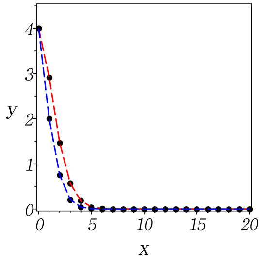
Figure 1: