Electricity price modeling and asset valuation: a multi-fuel structural approach

René Carmona Bendheim Center for Finance
Dept. ORFE, University of Princeton
Princeton NJ 08544, USA
rcarmona@princeton.edu
Michael Coulon ORFE
University of Princeton
Princeton NJ 08544, USA
mcoulon@princeton.edu
 and  Daniel Schwarz Oxford-Man Institute
University of Oxford
Oxford, UK
schwarz@maths.ox.ac.uk
Abstract.

We introduce a new and highly tractable structural model for spot and derivative prices in electricity markets. Using a stochastic model of the bid stack, we translate the demand for power and the prices of generating fuels into electricity spot prices. The stack structure allows for a range of generator efficiencies per fuel type and for the possibility of future changes in the merit order of the fuels. The derived spot price process captures important stylized facts of historical electricity prices, including both spikes and the complex dependence upon its underlying supply and demand drivers. Furthermore, under mild and commonly used assumptions on the distributions of the input factors, we obtain closed-form formulae for electricity forward contracts and for spark and dark spread options. As merit order dynamics and fuel forward prices are embedded into the model, we capture a much richer and more realistic dependence structure than can be achieved by classical reduced-form models. We illustrate these advantages by comparing with Margrabe’s formula and a simple cointegration model, and highlight important implications for the valuation of power plants.

JEL Classification Numbers: C60, G12, G13, Q40

Key words and phrases:
Electricity markets structural model forward prices spread options power plant valuation
Partially supported by NSF - DMS-0739195

1. Introduction

Since the onset of electricity market deregulation in the 1990s, the modeling of prices in these markets has become an important topic of research both in academia and industry. Energy companies own large portfolios of generation units and require sophisticated models of price dynamics in order to manage risk. Asset valuation is also of utmost importance in capital intensive industries and real option theory is typically used to associate the management of a plant to a string of spread options, spanning many years or decades. One of the main thrusts of this paper is to provide new and versatile tools for these valuations which efficiently capture the complex dependencies upon demand and production fuel prices.

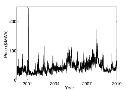
In electricity price modeling, important challenges include prominent seasonalities and mean-reversion at various time scales, sudden spikes and the strong link between the prices of electricity and other energy commodities (see Figures 1b and 5 for sample daily historical spot and forward prices from the PJM market) – features which mostly stem from the non-storability of electricity and the resulting matching of supply and demand at all times. While every model should attempt to capture these properties as well as possible, at the same time there is a need for fast and efficient methods to value power plants and other derivatives on the spot price. To achieve the latter goal of efficiency much literature has ignored or oversimplified the former goal of modeling structural relationships. In this paper, we propose a model that realistically captures the dependency of power prices on their primary drivers; yet we obtain closed-form expressions for spot, forward and option prices.

The existing literature on electricity price modeling can be approximately divided into three categories. At one end of the spectrum are so called full production cost models. These rely on knowledge of all generation units, their corresponding operational constraints and network transmission constraints. Prices are then typically solved for by complex optimization routines (cf. [19]). Although this type of model may provide market insights and forecasts in the short term, it is — due to its complexity — unsuited to handling uncertainty, and hence to derivative pricing or the valuation of physical assets. Other related approaches which share this weakness include models of strategic bidding (cf. [22]) and other equilibrium approaches (cf. [6]). At the other end of the spectrum are reduced form models. These are characterised by an exogenous specification of electricity prices, with either the forward curve (cf. [12] and [5]) or the spot price (cf. [16, 20, 4]) representing the starting point for the model. Reduced form models typically either ignore fuel prices or introduce them as exogenous correlated processes; hence they are not successful at capturing the important afore mentioned dependence structure between fuels and electricity. Further, spikes are usually only obtained through the inclusion of jump processes or regime switches, which provide little insight into the causes that underly these sudden price swings.

In between these two extremes is the structural approach to electricity price modeling, which stems from the seminal work of Barlow [3]. We use the adjective structural to describe models, which — to varying degrees of detail and complexity — explicitly approximate the supply curve in electricity markets (commonly known as the bid stack due to the price-setting auction). The market price is then obtained under the equilibrium assumption that demand and supply must match. In Barlow’s work the bid stack is simply a fixed parametric function, which is evaluated at a random demand level. Later works have refined the modeling of the bid curve and taken into account its dependency on the available capacity (cf. [8, 7, 10]), as well as fuel prices (cf. [27, 14, 1, 2]) and the cost of carbon emissions (cf. [23, 13]). The raison d’être of all structural models is very clear. If the bid curve is chosen appropriately, then observed stylized facts of historic data can be well matched. Moreover, because price formation is explained using fundamental variables and costs of production, these models offer insight into the causal relationships in the market; for example, prices in peak hours are most closely correlated with natural gas prices in markets with many gas ‘peaker’ plants; similarly, price spikes are typically observed to coincide with states of very high demand or low capacity. As a direct consequence, this class of models also performs best at capturing the varied dependencies between electricity, fuel prices, demand and capacity.

The model we propose falls into the category of structural models. Our work breaks from the current status quo by providing closed-form formulae for the prices of a number of derivative products in a market driven by two underlying fuels and featuring a continuum of efficiencies (heat rates). In the considered multi-fuel setting, our model of the bid stack allows the merit order to be dynamic: each fuel can become the marginal fuel and hence set the market price of electricity. Alternatively, several fuels can set the price jointly. Despite this complexity, under only mild assumptions on the distribution, under the pricing measure, of the terminal value of the processes representing electricity demand and fuels, we obtain explicit formulae for spot prices, forwards and spread options, as needed for power plant valuation. Moreover, our formulae capture very clearly and conveniently the dependency of electricity derivatives upon the prices of forward contracts written on the fuels that are used in the production process. This allows the model to easily ‘see’ additional information contained in the fuel forward curves, such as states of contango or backwardation — another feature, which distinguishes it from other approaches.

The parametrization of the bid stack we propose combines an exponential dependency on demand, suggested several times in the literature (cf. [30, 11, 24]), with the need for a heat rate function multiplicative in the fuel price, as stressed by Pirrong and Jermakyan [27]. Eydeland and Geman [18] propose a similar structure for forward prices and note that Black-Scholes like derivative prices are available if the power price is log-normal. However, this requires the assumption of a single marginal fuel type and ignores capacity limits. Coulon and Howison [14] construct the stack by approximating the distribution of the clusters of bids from each technology, but their approach relies heavily on numerical methods when it comes to derivative pricing. In the work of Aid et al [1], the authors simplify the stack construction by allowing only one heat rate (constant heat rate function) per fuel type, a significant oversimplification of spot price dynamics for mathematical convenience. Aid et al [2] extend this approach to improve spot price dynamics and capture spikes, but at the expense of a static merit order, ruling out, among other things, the possibility that coal and gas can change positions in the stack in the future. In both cases the results obtained by the authors only lead to semi-closed form formulae, which still have to be evaluated numerically.

The importance of the features incorporated in our model is supported by prominent developments observed in recent data. In particular, shale gas discoveries have led to a dramatic drop in US natural gas prices in recent years, from a high of over $13 in 2008 to under $3 in January 2012. Such a large price swing has rapidly pushed natural gas generators down the merit order, and highlights the need to account for uncertainty in future merit order changes, particularly for longer term problems like plant valuation. In addition, studying hourly data from 2004 to 2010 on marginal fuels in the PJM market (published by Monitoring Analytics), we observe that the electricity price was fully set by a single technology (only one marginal fuel) in only 16.1 per cent of the hours. For the year 2010 alone, the number drops to less than 5 per cent. Substantial overlap of bids from different fuels therefore exists, and changes in merit order occur gradually as prices move. We believe that our model of the bid stack adheres to many of the true features of the bid stack structure, which leads to a reliable reproduction of observed correlations and price dynamics, while retaining mathematical tractability.

2. Structural approach to electricity pricing

In the following we work on a complete probability space (Ω,,)Ω(\Omega,\mathcal{F},\mathbb{P}). For a fixed time horizon T+𝑇subscriptT\in\mathbb{R}_{+}, we define the (n+1)𝑛1(n+1)-dimensional standard Wiener process (Wt0,𝐖t)t[0,T]subscriptsubscriptsuperscript𝑊0𝑡subscript𝐖𝑡𝑡0𝑇(W^{0}_{t},\mathbf{W}_{t})_{t\in[0,T]}, where 𝐖:=(W1,,Wn)assign𝐖superscript𝑊1superscript𝑊𝑛\mathbf{W}:=(W^{1},\ldots,W^{n}). Let 0:=(t0)assignsuperscript0subscriptsuperscript0𝑡\mathcal{F}^{0}:=(\mathcal{F}^{0}_{t}) denote the filtration generated by W0superscript𝑊0W^{0} and W:=(tW)assignsuperscript𝑊subscriptsuperscript𝑊𝑡\mathcal{F}^{W}:=(\mathcal{F}^{W}_{t}) the filtration generated by 𝐖𝐖\mathbf{W}. Further, we define the market filtration :=0Wassignsuperscript0superscript𝑊\mathcal{F}:=\mathcal{F}^{0}\vee\mathcal{F}^{W}. All relationships between random variables are to be understood in the almost surely sense.

2.1. Price Setting in Electricity Markets

We consider a market in which individual firms generate electricity. All firms submit day-ahead bids to a central market administrator, whose task it is to allocate the production of electricity amongst them. Each firm’s bids take the form of price-quantity pairs representing an amount of electricity the firm is willing to produce, and the price at which the firm is willing to sell it111Alternatively, firms may, in some markets, submit continuous bid curves, which map an amount of electricity to the price at which it is offered. For our purposes this distinction will however not be relevant.. An important part is therefore played by the merit order, a rule by which cheaper production units are called upon before more expensive ones in the electricity generation process. This ultimately guarantees that electricity is supplied at the lowest possible price.222This description is of course a simplification of the market administrator’s complicated unit commitment problem, typically solved by optimization in order to satisfy various operational constraints of generators, as well as transmission constraints. Details vary from market to market and we do not address these issues here, as our goal is to approximate the price setting mechanism and capture the key relationships needed for derivative pricing.

Assumption 1.

The market administrator arranges bids according to the merit order and hence in increasing order of costs of production.

We refer to the resulting map from the total supply of electricity and the factors that influence the bid levels to the price of the marginal unit as the market bid stack and assume that it can be represented by a measurable function

b:[0,ξ¯]×n(ξ,𝐬)b(ξ,𝐬),:𝑏contains0¯𝜉superscript𝑛𝜉𝐬𝑏𝜉𝐬b:[0,\bar{\xi}]\times\mathbb{R}^{n}\ni(\xi,\mathbf{s})\hookrightarrow b(\xi,\mathbf{s})\in\mathbb{R},

which will be assumed to be strictly increasing in its first variable. Here, ξ¯+¯𝜉subscript\bar{\xi}\in\mathbb{R}_{+} represents the combined capacity of all generators in the market, henceforth the market capacity (measured in MW), and 𝐬n𝐬superscript𝑛\mathbf{s}\in\mathbb{R}^{n} represents factors of production which drive firm bids (e.g. fuel prices).

Demand for electricity is assumed to be price-inelastic and given exogenously by an t0subscriptsuperscript0𝑡\mathcal{F}^{0}_{t}-adapted process (Dt)subscript𝐷𝑡(D_{t}) (measured in MW). As we shall see later, the prices of the factors of production used in the electricity generation process will be assumed to be tWsubscriptsuperscript𝑊𝑡\mathcal{F}^{W}_{t}-adapted. So under the objective historical measure \mathbb{P}, the demand is statistically independent of these prices. This is a reasonable assumption as power demand is typically driven predominantly by temperature, which fluctuates at a faster time scale and depends more on local or regional conditions than fuel prices. The market responds to this demand by supplying an amount ξt[0,ξ¯]subscript𝜉𝑡0¯𝜉\xi_{t}\in[0,\bar{\xi}] of electricity. We assume that the market is in equilibrium with respect to the supply of and demand for electricity; i.e.

(1) Dt=ξt,for t[0,T].formulae-sequencesubscript𝐷𝑡subscript𝜉𝑡for 𝑡0𝑇D_{t}=\xi_{t},\quad\text{for }t\in[0,T].

This implies that Dt[0,ξ¯]subscript𝐷𝑡0¯𝜉D_{t}\in[0,\bar{\xi}] for t[0,T]𝑡0𝑇t\in[0,T] and (ξt)subscript𝜉𝑡(\xi_{t}) is t0subscriptsuperscript0𝑡\mathcal{F}^{0}_{t}-adapted.

The market price of electricity (Pt)subscript𝑃𝑡(P_{t}) is now defined as the price at which the last unit that is needed to satisfy demand sells its electricity; i.e. using (1),

(2) Pt:=b(Dt,),for t[0,T].formulae-sequenceassignsubscript𝑃𝑡𝑏subscript𝐷𝑡for 𝑡0𝑇P_{t}:=b(D_{t},\cdot),\quad\text{for }t\in[0,T].

We emphasize the different roles played by the first variable (i.e. demand) and all subsequent variables (i.e. factors driving bid levels) of the bid stack function b𝑏b. Due to the inelasticity assumption, the level of demand fully determines the quantity of electricity that is being generated; all subsequent variables merely impact the merit order arrangement of the bids.

Remark 1.

The price setting mechanism described above applies directly to day-ahead spot prices set by uniform auctions, as in most exchanges today. However, we believe that in a competitive market with rational agents, the day-ahead auction price also serves as the key reference point for real-time and over-the-counter prices.

2.2. Mathematical Model of the Bid Stack

From the previous subsection, it is clear that the price of electricity in a structural model like the one we are proposing depends critically on the construction of the function b𝑏b. Before we explain how this is done in the current setting, we make the following assumption about the formation of firms’ bids.

Assumption 2.

Bids are driven by production costs. Furthermore,

  1. (1)

    costs depend on fuel prices and firm-specific characteristics only;

  2. (2)

    firms’ marginal costs are strictly increasing.
Refer to caption
(a) Sample bid stacks.
Refer to caption
(b) Historical daily average prices.
Figure 1. Historical prices and bids from the PJM market in the North East US

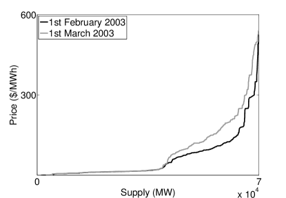
To back up Assumption 2, we briefly consider it in light of historic bid and spot price data. Figure 1a plots the bid stack from the PJM market region in the US on the first day of two consecutive months. Firstly, rapidly increasing marginal costs lead to the steep slope of the stack near the market capacity (70,000 MW); this feature translates directly into spikes in spot prices (see Figure 1b) when demand is high. Between the two sample dates in February and March 2003, the prices of gas increased rapidly. In the PJM market gas fired plants have historically featured mainly in the second half of the bid stack. Therefore, it is precisely the gas price related increase in production costs, which explains the increase in bid levels observed beyond about 40,000MW in Figure 1a (see also §4.2 for a discussion of recent merit order changes).

Production costs are typically linked to a particular fuel price (e.g. coal, natural gas, lignite, oil, etc.). Furthermore, within each fuel class, the cost of production may vary significantly, for example as old generators may have a higher heat rate (lower efficiency) than new units. It is not our aim to provide a mathematical model that explains how to aggregate individual bids or capture strategic bidding. Instead, we group together generators of the same fuel type and assume the resulting bid curve to be exogenously given and to satisfy Assumption 2. From this set of bid curves, the merit order rule then determines the construction of the market bid stack.

Let I={1,,n}𝐼1𝑛I=\{1,\ldots,n\} denote the index set of all the fuels used in the market to generate electricity. We assume that their prices are the only factors influencing the bid stacks. With each iI𝑖𝐼i\in I we associate an tWsubscriptsuperscript𝑊𝑡\mathcal{F}^{W}_{t}-adapted fuel price process (Sti)subscriptsuperscript𝑆𝑖𝑡(S^{i}_{t}) and we define the fuel bid curve for fuel i𝑖i to be a measurable function

bi:[0,ξ¯i]×(ξ,s)bi(ξ,s),:subscript𝑏𝑖contains0subscript¯𝜉𝑖𝜉𝑠subscript𝑏𝑖𝜉𝑠b_{i}:[0,\bar{\xi}_{i}]\times\mathbb{R}\ni(\xi,s)\hookrightarrow b_{i}(\xi,s)\in\mathbb{R},

where the argument ξ𝜉\xi represents the amount of electricity supplied by generators utilizing fuel type i𝑖i, s𝑠s a possible value of the price Stisubscriptsuperscript𝑆𝑖𝑡S^{i}_{t}, and ξ¯i+superscript¯𝜉𝑖subscript\bar{\xi}^{i}\in\mathbb{R}_{+} the aggregate capacity of all the generators utilizing fuel type i𝑖i. We assume that bisubscript𝑏𝑖b_{i} is strictly increasing in its first argument, as required by Assumption 2. Further, also for iI𝑖𝐼i\in I, let the tsubscript𝑡\mathcal{F}_{t}-adapted process (ξti)subscriptsuperscript𝜉𝑖𝑡(\xi^{i}_{t}) represent the amount of electricity supplied by generators utilizing fuel type i𝑖i. It follows that

iIξ¯i=ξ¯,andDt=iIξti,for t[0,T].formulae-sequencesubscript𝑖𝐼superscript¯𝜉𝑖¯𝜉andformulae-sequencesubscript𝐷𝑡subscript𝑖𝐼subscriptsuperscript𝜉𝑖𝑡for 𝑡0𝑇\sum_{i\in I}\bar{\xi}^{i}=\bar{\xi},\quad\text{and}\quad D_{t}=\sum_{i\in I}\xi^{i}_{t},\quad\text{for }t\in[0,T].

In order to simplify the notation below, for iI𝑖𝐼i\in I, and for each s𝑠s\in\mathbb{R} we denote by bi(,s)1subscript𝑏𝑖superscript𝑠1b_{i}(\,\cdot\,,s)^{-1} the generalized (right continuous) inverse of the function ξbi(ξ,s)𝜉subscript𝑏𝑖𝜉𝑠\xi\hookrightarrow b_{i}(\xi,s). Thus

bi(,s)1(p):=ξ¯iinf{ξ(0,ξ¯i]:bi(ξ,s)>p},for (p,s)×,formulae-sequenceassignsubscript𝑏𝑖superscript𝑠1𝑝superscript¯𝜉𝑖infimumconditional-set𝜉0superscript¯𝜉𝑖subscript𝑏𝑖𝜉𝑠𝑝for 𝑝𝑠b_{i}(\,\cdot\,,s)^{-1}(p):=\bar{\xi}^{i}\wedge\inf\left\{\xi\in(0,\bar{\xi}^{i}]:\,b_{i}(\xi,s)>p\right\},\quad\text{for }(p,s)\in\mathbb{R}\times\mathbb{R},

where we use the standard convention inf=+infimum\inf\emptyset=+\infty. Using the notation

b¯i(s):=bi(0,s)andb¯i(s):=bi(ξ¯i,s)formulae-sequenceassignsubscript¯𝑏𝑖𝑠subscript𝑏𝑖0𝑠andassignsubscript¯𝑏𝑖𝑠subscript𝑏𝑖superscript¯𝜉𝑖𝑠\underline{b}_{i}(s):=b_{i}(0,s)\quad\text{and}\quad\bar{b}_{i}(s):=b_{i}(\bar{\xi}^{i},s)

and writing b^i1(p,s)=bi(,s)1(p)superscriptsubscript^𝑏𝑖1𝑝𝑠subscript𝑏𝑖superscript𝑠1𝑝\hat{b}_{i}^{-1}(p,s)=b_{i}(\,\cdot\,,s)^{-1}(p) to ease the notation, we see that b^i1(p,s)=0superscriptsubscript^𝑏𝑖1𝑝𝑠0\hat{b}_{i}^{-1}(p,s)=0 if p(,b¯i(s))𝑝subscript¯𝑏𝑖𝑠p\in(-\infty,\underline{b}_{i}(s)), b^i1(p,s)=ξ¯isuperscriptsubscript^𝑏𝑖1𝑝𝑠superscript¯𝜉𝑖\hat{b}_{i}^{-1}(p,s)=\bar{\xi}^{i} if p[b¯i(s),)𝑝subscript¯𝑏𝑖𝑠p\in[\bar{b}_{i}(s),\infty), and b^i1(p,s)[0,ξ¯i]superscriptsubscript^𝑏𝑖1𝑝𝑠0superscript¯𝜉𝑖\hat{b}_{i}^{-1}(p,s)\in[0,\bar{\xi}^{i}] if p[b¯i(s),b¯i(s))𝑝subscript¯𝑏𝑖𝑠subscript¯𝑏𝑖𝑠p\in[\underline{b}_{i}(s),\bar{b}_{i}(s)). For fuel iI𝑖𝐼i\in I at price Sti=ssubscriptsuperscript𝑆𝑖𝑡𝑠S^{i}_{t}=s and for electricity prices below b¯i(s)subscript¯𝑏𝑖𝑠\underline{b}_{i}(s) no capacity from the i𝑖ith technology will be available. Similarly, once all resources from a technology are exhausted, increases in the electricity price will not lead to further production units being brought online. So defined, the inverse function b^i1superscriptsubscript^𝑏𝑖1\hat{b}_{i}^{-1} maps a given price of electricity and the price of fuel i𝑖i to the amount of electricity supplied by generators relying on this fuel type.

Proposition 1.

For a given vector (Dt,𝐒t)subscript𝐷𝑡subscript𝐒𝑡(D_{t},\mathbf{S}_{t}), where 𝐒t:=(St1,,Stn)assignsubscript𝐒𝑡subscriptsuperscript𝑆1𝑡subscriptsuperscript𝑆𝑛𝑡\mathbf{S}_{t}:=(S^{1}_{t},\ldots,S^{n}_{t}), the market price of electricity (Pt)subscript𝑃𝑡(P_{t}) is determined by

(3) Pt=miniIb¯i(Sti)sup{p:iIb^i1(p,Sti)<Dt},for t[0,T].formulae-sequencesubscript𝑃𝑡subscript𝑖𝐼subscript¯𝑏𝑖subscriptsuperscript𝑆𝑖𝑡supremumconditional-set𝑝subscript𝑖𝐼superscriptsubscript^𝑏𝑖1𝑝subscriptsuperscript𝑆𝑖𝑡subscript𝐷𝑡for 𝑡0𝑇P_{t}=\min_{i\in I}\underline{b}_{i}\left(S^{i}_{t}\right)\vee\sup\left\{p\in\mathbb{R}:\sum_{i\in I}\hat{b}_{i}^{-1}\left(p,S^{i}_{t}\right)<D_{t}\right\},\quad\text{for }t\in[0,T].
Proof.

By the definition of b^i1superscriptsubscript^𝑏𝑖1\hat{b}_{i}^{-1}, the function b~1superscript~𝑏1\tilde{b}^{-1}, defined by

b~1(p,s1,,sn):=iIb^i1(p,si),assignsuperscript~𝑏1𝑝superscript𝑠1superscript𝑠𝑛subscript𝑖𝐼superscriptsubscript^𝑏𝑖1𝑝superscript𝑠𝑖\tilde{b}^{-1}(p,s^{1},\cdots,s^{n}):=\sum_{i\in I}\hat{b}_{i}^{-1}(p,s^{i}),

is, when the prices of all the fuels are fixed, a non-decreasing map taking the electricity price to the corresponding amount of electricity generated by the market. Similarly to the case of one fixed fuel price, for each fixed set of fuel prices, say 𝐬:=(s1,,sn)assign𝐬superscript𝑠1superscript𝑠𝑛\mathbf{s}:=(s^{1},\cdots,s^{n}), we define the bid stack function ξb(ξ,𝐬)𝜉𝑏𝜉𝐬\xi\hookrightarrow b(\xi,\mathbf{s}) as the generalized (left continuous) inverse of the function ξb~1(p,s1,,sn)𝜉superscript~𝑏1𝑝superscript𝑠1superscript𝑠𝑛\xi\hookrightarrow\tilde{b}^{-1}(p,s^{1},\cdots,s^{n}) defined above, namely

b(ξ,𝐬):=miniIb¯i(si)sup{p:iIb^i1(p,si)<ξ},for (ξ,𝐬)[0,ξ¯]×n,formulae-sequenceassign𝑏𝜉𝐬subscript𝑖𝐼subscript¯𝑏𝑖superscript𝑠𝑖supremumconditional-set𝑝subscript𝑖𝐼superscriptsubscript^𝑏𝑖1𝑝superscript𝑠𝑖𝜉for 𝜉𝐬0¯𝜉superscript𝑛b(\xi,\mathbf{s}):=\min_{i\in I}\underline{b}_{i}\left(s^{i}\right)\vee\sup\left\{p\in\mathbb{R}:\sum_{i\in I}\hat{b}_{i}^{-1}\left(p,s^{i}\right)<\xi\right\},\quad\text{for }(\xi,\mathbf{s})\in[0,\bar{\xi}]\times\mathbb{R}^{n},

where we use the convention sup=supremum\sup\emptyset=-\infty.

The desired result follows from the definition of the market price of electricity in (2). ∎

2.3. Defining a Pricing Measure in the Structural Setting

The results presented in this paper do not depend on a particular model for the evolution of the demand for electricity and the prices of fuels. In particular, the concrete bid stack model for the electricity spot price introduced in §3 is simply a deterministic function of the exogenously given factors under the real world measure \mathbb{P}. However, for the pricing of derivatives in §4 and §5 we need to define a pricing measure \mathbb{Q} and the distribution of the random factors at maturity under this new measure will be important for the results that we obtain later.

For an tsubscript𝑡\mathcal{F}_{t}-adapted process 𝜽tsubscript𝜽𝑡\bm{\theta}_{t}, where 𝜽t:=(θt0,θt1,,θtn)assignsubscript𝜽𝑡subscriptsuperscript𝜃0𝑡subscriptsuperscript𝜃1𝑡subscriptsuperscript𝜃𝑛𝑡\bm{\theta}_{t}:=(\theta^{0}_{t},\theta^{1}_{t},\ldots,\theta^{n}_{t}), a measure 𝒬similar-to𝒬\mathcal{Q}\sim\mathbb{P} is characterized by the Radon-Nikodym derivative

(4) d𝒬d:=exp(0T𝜽ud𝐖u120T|𝜽u|2du),assignd𝒬dsuperscriptsubscript0𝑇subscript𝜽𝑢differential-dsubscript𝐖𝑢12superscriptsubscript0𝑇superscriptsubscript𝜽𝑢2differential-d𝑢\frac{\mathrm{d}\mathcal{Q}}{\mathrm{d}\mathbb{P}}:=\exp\left(-\int_{0}^{T}\bm{\theta}_{u}\cdot\ \mathrm{d}\mathbf{W}_{u}-\frac{1}{2}\int_{0}^{T}\left|\bm{\theta}_{u}\right|^{2}\ \mathrm{d}u\right),

where we assume that (𝜽t)subscript𝜽𝑡(\bm{\theta}_{t}) satisfies the so-called Novikov condition

𝔼[exp(120T|𝜽u|2du)]<.𝔼delimited-[]12superscriptsubscript0𝑇superscriptsubscript𝜽𝑢2differential-d𝑢\mathbb{E}\left[\exp\left(\frac{1}{2}\int_{0}^{T}\left|\bm{\theta}_{u}\right|^{2}\ \mathrm{d}u\right)\right]<\infty.

We identify (θt0)subscriptsuperscript𝜃0𝑡(\theta^{0}_{t}) and (θti)subscriptsuperscript𝜃𝑖𝑡(\theta^{i}_{t}) with the market prices of risk for demand and for fuel i𝑖i respectively. We choose to avoid the difficulties of estimating the market price of risk (see for example [19] for several possibilities) and instead make the following assumption.

Assumption 3.

The market chooses a pricing measure similar-to\mathbb{Q}\sim\mathbb{P}, such that

{𝒬:all discounted prices of traded assets are local 𝒬-martingales}.conditional-setsimilar-to𝒬all discounted prices of traded assets are local 𝒬-martingales\mathbb{Q}\in\left\{\mathcal{Q}\sim\mathbb{P}:\text{all discounted prices of traded assets are local $\mathcal{Q}$-martingales}\right\}.

Note that we make no assumption regarding market completeness here. Because of the non-storability condition, certainly electricity cannot be considered a traded asset. Further, there are different approaches to modeling fuel prices; they may be treated as traded assets (hence local martingales under \mathbb{Q}) or — more realistically — assumed to exhibit mean reversion under the pricing measure. Either way, demand is a fundamental factor and the noise (Wt0)subscriptsuperscript𝑊0𝑡(W^{0}_{t}) associated with it means that the joined market of fuels and electricity is bound to be incomplete. Note however, that all derivative products that we price later in the paper (forward contracts and spread options) are clearly traded assets and covered by Assumption 3.

3. Exponential Bid Stack Model

Equation (3) in general cannot be solved explicitly. The reason for this is that any explicit solution essentially requires the inversion of the sum of inverses of individual fuel bid curves.

We now propose a specific form for the individual fuel bid curves, which allows us to obtain a closed form solution for the market bid stack b𝑏b. Here and throughout the rest of the paper, for iI𝑖𝐼i\in I, we define bisubscript𝑏𝑖b_{i} to be explicitly given by

(5) bi(ξ,s):=sexp(ki+miξ),for (ξ,s)[0,ξ¯i]×+,formulae-sequenceassignsubscript𝑏𝑖𝜉𝑠𝑠subscript𝑘𝑖subscript𝑚𝑖𝜉for 𝜉𝑠0superscript¯𝜉𝑖subscriptb_{i}(\xi,s):=s\exp(k_{i}+m_{i}\xi),\quad\text{for }(\xi,s)\in[0,\bar{\xi}^{i}]\times\mathbb{R}_{+},

where kisubscript𝑘𝑖k_{i} and misubscript𝑚𝑖m_{i} are constants and misubscript𝑚𝑖m_{i} is strictly positive. Note that bisubscript𝑏𝑖b_{i} clearly satisfies (1) and since it is strictly increasing on its domain of definition it also satisfies (2).

3.1. The Case of n𝑛n Fuels

For observed (Dt,𝐒t)subscript𝐷𝑡subscript𝐒𝑡(D_{t},\mathbf{S}_{t}), let us define the sets M,CI𝑀𝐶𝐼M,C\subseteq I by

M𝑀\displaystyle M :={iI:generators using fuel i are partially used}assignabsentconditional-set𝑖𝐼generators using fuel i are partially used\displaystyle:=\left\{i\in I:\text{generators using fuel $i$ are partially used}\right\}
andCand𝐶\displaystyle\text{and}\quad C :={iI:the entire capacity ξ¯i of generators using fuel i is used}.assignabsentconditional-set𝑖𝐼the entire capacity ξ¯i of generators using fuel i is used\displaystyle:=\left\{i\in I:\text{the entire capacity $\bar{\xi}^{i}$ of generators using fuel $i$ is used}\right\}.

A possible procedure for establishing the members of M𝑀M and C𝐶C is to order all the values of b¯isubscript¯𝑏𝑖\underline{b}_{i} and b¯isubscript¯𝑏𝑖\bar{b}_{i} and determine the corresponding cumulative amounts of electricity that are supplied at these prices. Then find where demand lies in this ordering.

With the above definition of M𝑀M and C𝐶C we arrive at the following corollary to Proposition 1.

Corollary 1.

For bisubscript𝑏𝑖b_{i} of exponential form, as defined in (5), the market price of electricity is given explicitly by the left continuous version of

(6) Pt=(iM(Sti)αi)exp{β+γ(DtiCξ¯i)},for t[0,T],formulae-sequencesubscript𝑃𝑡subscriptproduct𝑖𝑀superscriptsubscriptsuperscript𝑆𝑖𝑡subscript𝛼𝑖𝛽𝛾subscript𝐷𝑡subscript𝑖𝐶superscript¯𝜉𝑖for 𝑡0𝑇P_{t}=\left(\prod_{i\in M}\left(S^{i}_{t}\right)^{\alpha_{i}}\right)\exp\left\{\beta+\gamma\left(D_{t}-\sum_{i\in C}\bar{\xi}^{i}\right)\right\},\quad\text{for }t\in[0,T],

where

αi:=1ζ(jM,jimj),β:=1ζ(lMkljM,jlmj),formulae-sequenceassignsubscript𝛼𝑖1𝜁subscriptproductformulae-sequence𝑗𝑀𝑗𝑖subscript𝑚𝑗assign𝛽1𝜁subscript𝑙𝑀subscript𝑘𝑙subscriptproductformulae-sequence𝑗𝑀𝑗𝑙subscript𝑚𝑗\displaystyle\alpha_{i}:=\frac{1}{\zeta}\left(\prod_{j\in M,j\neq i}m_{j}\right),\quad\beta:=\frac{1}{\zeta}\left(\sum_{l\in M}k_{l}\prod_{j\in M,j\neq l}m_{j}\right),
γ:=1ζ(jMmj)andζ:=lMjM,jlmj.formulae-sequenceassign𝛾1𝜁subscriptproduct𝑗𝑀subscript𝑚𝑗andassign𝜁subscript𝑙𝑀subscriptproductformulae-sequence𝑗𝑀𝑗𝑙subscript𝑚𝑗\displaystyle\gamma:=\frac{1}{\zeta}\left(\prod_{j\in M}m_{j}\right)\quad\text{and}\quad\zeta:=\sum_{l\in M}\prod_{j\in M,j\neq l}m_{j}.
Proof.

At any time t[0,T]𝑡0𝑇t\in[0,T] the electricity price depends on the composition of the sets M𝑀M and C𝐶C; i.e. the current set of marginal and fully utilized fuel types.

For iM𝑖𝑀i\in M, b^i1=bi1superscriptsubscript^𝑏𝑖1superscriptsubscript𝑏𝑖1\hat{b}_{i}^{-1}=b_{i}^{-1}, for iC𝑖𝐶i\in C, b^i1=ξ¯isuperscriptsubscript^𝑏𝑖1superscript¯𝜉𝑖\hat{b}_{i}^{-1}=\bar{\xi}^{i} and for iI{MC}𝑖𝐼𝑀𝐶i\in I\setminus\{M\cup C\}, b^i1=0superscriptsubscript^𝑏𝑖10\hat{b}_{i}^{-1}=0. Therefore, inside the supremum in (3), we replace I𝐼I with M𝑀M and take iCξ¯isubscript𝑖𝐶superscript¯𝜉𝑖\sum_{i\in C}\bar{\xi}^{i} to the right hand side. By Proposition 1 the electricity price is given by the left continuous inverse of the function iMb^i1subscript𝑖𝑀superscriptsubscript^𝑏𝑖1\sum_{i\in M}\hat{b}_{i}^{-1}, which in the exponential case under consideration, simplifies to a single log\log function and yields (6). ∎

Refer to caption
(a) Fuel bid curves bisubscript𝑏𝑖b_{i}.
Refer to caption
(b) Market bid stack b𝑏b.
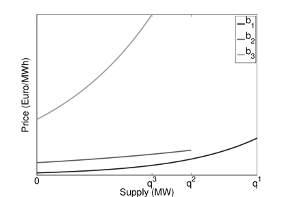
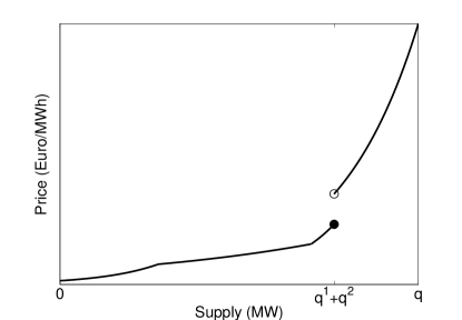
Figure 2. Example of fuel bid curves and resulting market bid stack for I:={1,2,3},q:=ξ¯formulae-sequenceassign𝐼123assign𝑞¯𝜉I:=\{1,2,3\},\ q:=\bar{\xi}

It is clear from equation (6) that the number of possible expressions for the electricity price is fully determined by the different configurations the sets M𝑀M and C𝐶C can take. In fact, fluctuations in demand and fuel prices can lead to

(7) i=1n(ni)[j=0ni(nij)]superscriptsubscript𝑖1𝑛𝑛𝑖delimited-[]superscriptsubscript𝑗0𝑛𝑖𝑛𝑖𝑗\sum_{i=1}^{n}\left(\begin{array}[]{c}n\\ i\end{array}\right)\left[\sum_{j=0}^{n-i}\left(\begin{array}[]{c}n-i\\ j\end{array}\right)\right]

distinct cases for (6). Nonetheless, the market bid stack is always a piece-wise exponential function of demand (see Figure 2) with constantly evolving shape as fuel prices move. This captures in a very tractable way the influence of fuel prices on the merit order and resulting power price dynamics.

3.2. The Case of Two Fuels

For the remainder of the paper, we restrict our attention to the case of a two-fuel market, consisting of coal and natural gas generators. Our results can in principle be extended to the general case of n>2𝑛2n>2 fuels. However, the level of complexity of the formulas increases rapidly, as evidenced by the number of possible expressions given in (7). We also choose to omit the analysis of the one fuel case, which leads to far simpler expressions throughout, but cannot lead to merit order changes. From now on, we set I:={c,g}assign𝐼𝑐𝑔I:=\{c,g\} and carry over all notation introduced in §2 and §3 so far.

From (7) we know that there are five possible expressions for the electricity spot price. We list them in Table 1. Note that fixing Dtsubscript𝐷𝑡D_{t} reduces this list to some subset of three, each of which — depending on the state of 𝐒tsubscript𝐒𝑡\mathbf{S}_{t} — can set the electricity price. (A similar reduction to three expressions occurs by fixing 𝐒tsubscript𝐒𝑡\mathbf{S}_{t}.) We exploit this property to write formula (6) in a form more amenable to calculations, identifying all cases explicitly.

Ptsubscript𝑃𝑡P_{t}, for t[0,T]𝑡0𝑇t\in[0,T] Criterion Composition of
M𝑀M C𝐶C
Stcexp(kc+mcDt)subscriptsuperscript𝑆𝑐𝑡subscript𝑘𝑐subscript𝑚𝑐subscript𝐷𝑡S^{c}_{t}\exp\left(k_{c}+m_{c}D_{t}\right) bc(Dt,Stc)b¯g(Stg)subscript𝑏𝑐subscript𝐷𝑡subscriptsuperscript𝑆𝑐𝑡subscript¯𝑏𝑔subscriptsuperscript𝑆𝑔𝑡b_{c}\left(D_{t},S^{c}_{t}\right)\leq\underline{b}_{g}\left(S^{g}_{t}\right) {c}𝑐\{c\} {}\{\varnothing\}
Stgexp(kg+mgDt)subscriptsuperscript𝑆𝑔𝑡subscript𝑘𝑔subscript𝑚𝑔subscript𝐷𝑡S^{g}_{t}\exp\left(k_{g}+m_{g}D_{t}\right) bg(Dt,Stg)b¯c(Stc)subscript𝑏𝑔subscript𝐷𝑡subscriptsuperscript𝑆𝑔𝑡subscript¯𝑏𝑐subscriptsuperscript𝑆𝑐𝑡b_{g}\left(D_{t},S^{g}_{t}\right)\leq\underline{b}_{c}\left(S^{c}_{t}\right) {g}𝑔\{g\} {}\{\varnothing\}
Stcexp(kc+mc(Dtξ¯g))subscriptsuperscript𝑆𝑐𝑡subscript𝑘𝑐subscript𝑚𝑐subscript𝐷𝑡superscript¯𝜉𝑔S^{c}_{t}\exp\left(k_{c}+m_{c}\left(D_{t}-\bar{\xi}^{g}\right)\right) bc(Dtξ¯g,Stc)>b¯g(Stg)subscript𝑏𝑐subscript𝐷𝑡superscript¯𝜉𝑔subscriptsuperscript𝑆𝑐𝑡subscript¯𝑏𝑔subscriptsuperscript𝑆𝑔𝑡b_{c}\left(D_{t}-\bar{\xi}^{g},S^{c}_{t}\right)>\bar{b}_{g}\left(S^{g}_{t}\right) {c}𝑐\{c\} {g}𝑔\{g\}
Stgexp(kg+mg(Dtξ¯c))subscriptsuperscript𝑆𝑔𝑡subscript𝑘𝑔subscript𝑚𝑔subscript𝐷𝑡superscript¯𝜉𝑐S^{g}_{t}\exp\left(k_{g}+m_{g}\left(D_{t}-\bar{\xi}^{c}\right)\right) bg(Dtξ¯c,Stg)>b¯c(Stc)subscript𝑏𝑔subscript𝐷𝑡superscript¯𝜉𝑐subscriptsuperscript𝑆𝑔𝑡subscript¯𝑏𝑐subscriptsuperscript𝑆𝑐𝑡b_{g}\left(D_{t}-\bar{\xi}^{c},S^{g}_{t}\right)>\bar{b}_{c}\left(S^{c}_{t}\right) {g}𝑔\{g\} {c}𝑐\{c\}
(Stc)αc(Stg)αgexp(β+γDt)superscriptsubscriptsuperscript𝑆𝑐𝑡subscript𝛼𝑐superscriptsubscriptsuperscript𝑆𝑔𝑡subscript𝛼𝑔𝛽𝛾subscript𝐷𝑡\left(S^{c}_{t}\right)^{\alpha_{c}}\left(S^{g}_{t}\right)^{\alpha_{g}}\exp\left(\beta+\gamma D_{t}\right) otherwise {c,g}𝑐𝑔\{c,g\} {}\{\varnothing\}
Table 1. Distinct cases for the electricity price (6) in the two fuel case

To simplify the presentation in the text below, we define

bcg(ξ,𝐬):=(sc)αc(sg)αgexp(β+γξ),for (ξ,𝐬)[0,ξ¯]×+2,formulae-sequenceassignsubscript𝑏𝑐𝑔𝜉𝐬superscriptsuperscript𝑠𝑐subscript𝛼𝑐superscriptsuperscript𝑠𝑔subscript𝛼𝑔𝛽𝛾𝜉for 𝜉𝐬0¯𝜉superscriptsubscript2b_{cg}\left(\xi,\mathbf{s}\right):=\left(s^{c}\right)^{\alpha_{c}}\left(s^{g}\right)^{\alpha_{g}}\exp\left(\beta+\gamma\xi\right),\quad\text{for }\left(\xi,\mathbf{s}\right)\in[0,\bar{\xi}]\times\mathbb{R}_{+}^{2},

where αcsubscript𝛼𝑐\alpha_{c}, αgsubscript𝛼𝑔\alpha_{g}, β𝛽\beta and γ𝛾\gamma are defined in Corollary 1 and simplify for two fuels to

αc=mgmc+mg,αg=1αc=mcmc+mg,β=kcmg+kgmcmc+mg,γ=mcmgmc+mg.formulae-sequenceformulae-sequencesubscript𝛼𝑐subscript𝑚𝑔subscript𝑚𝑐subscript𝑚𝑔subscript𝛼𝑔1subscript𝛼𝑐subscript𝑚𝑐subscript𝑚𝑐subscript𝑚𝑔formulae-sequence𝛽subscript𝑘𝑐subscript𝑚𝑔subscript𝑘𝑔subscript𝑚𝑐subscript𝑚𝑐subscript𝑚𝑔𝛾subscript𝑚𝑐subscript𝑚𝑔subscript𝑚𝑐subscript𝑚𝑔\alpha_{c}=\frac{m_{g}}{m_{c}+m_{g}},\quad\alpha_{g}=1-\alpha_{c}=\frac{m_{c}}{m_{c}+m_{g}},\quad\beta=\frac{k_{c}m_{g}+k_{g}m_{c}}{m_{c}+m_{g}},\quad\gamma=\frac{m_{c}m_{g}}{m_{c}+m_{g}}.

Further, we set i:=argmin{ξ¯c,ξ¯g}assignsubscript𝑖argminsuperscript¯𝜉𝑐superscript¯𝜉𝑔i_{-}:=\operatornamewithlimits{argmin}\left\{\bar{\xi}^{c},\bar{\xi}^{g}\right\} and i+:=argmax{ξ¯c,ξ¯g}assignsubscript𝑖argmaxsuperscript¯𝜉𝑐superscript¯𝜉𝑔i_{+}:=\operatornamewithlimits{argmax}\left\{\bar{\xi}^{c},\bar{\xi}^{g}\right\}.

Corollary 2.

With I:={c,g}assign𝐼𝑐𝑔I:=\{c,g\}, for t[0,T]𝑡0𝑇t\in[0,T], the electricity spot price is given by

Pt=blow(Dt,𝐒t)𝕀[0,ξ¯i](Dt)+bmid(Dt,𝐒t)𝕀(ξ¯i,ξ¯i+](Dt)+bhigh(Dt,𝐒t)𝕀(ξ¯i+,ξ¯](Dt),subscript𝑃𝑡subscript𝑏lowsubscript𝐷𝑡subscript𝐒𝑡subscript𝕀0superscript¯𝜉subscript𝑖subscript𝐷𝑡subscript𝑏midsubscript𝐷𝑡subscript𝐒𝑡subscript𝕀superscript¯𝜉subscript𝑖superscript¯𝜉subscript𝑖subscript𝐷𝑡subscript𝑏highsubscript𝐷𝑡subscript𝐒𝑡subscript𝕀superscript¯𝜉subscript𝑖¯𝜉subscript𝐷𝑡P_{t}=b_{\text{low}}\left(D_{t},\mathbf{S}_{t}\right)\mathbb{I}_{\left[0,\bar{\xi}^{i_{-}}\right]}(D_{t})+b_{\text{mid}}\left(D_{t},\mathbf{S}_{t}\right)\mathbb{I}_{\left(\bar{\xi}^{i_{-}},\bar{\xi}^{i_{+}}\right]}(D_{t})+b_{\text{high}}\left(D_{t},\mathbf{S}_{t}\right)\mathbb{I}_{\left(\bar{\xi}^{i_{+}},\bar{\xi}\right]}(D_{t}),

where, for (ξ,𝐬)[0,ξ¯]×+2𝜉𝐬0¯𝜉superscriptsubscript2(\xi,\mathbf{s})\in[0,\bar{\xi}]\times\mathbb{R}_{+}^{2},

blow(ξ,𝐬):=bc(ξ,sc)𝕀{bc(ξ,sc)<b¯g(sg)}+bg(ξ,sg)𝕀{bg(ξ,sg)<b¯c(sc)}+bcg(ξ,𝐬)𝕀{bc(ξ,sc)b¯g(sg),bg(ξ,sg)b¯c(sc)},assignsubscript𝑏low𝜉𝐬subscript𝑏𝑐𝜉superscript𝑠𝑐subscript𝕀subscript𝑏𝑐𝜉superscript𝑠𝑐subscript¯𝑏𝑔superscript𝑠𝑔subscript𝑏𝑔𝜉superscript𝑠𝑔subscript𝕀subscript𝑏𝑔𝜉superscript𝑠𝑔subscript¯𝑏𝑐superscript𝑠𝑐subscript𝑏𝑐𝑔𝜉𝐬subscript𝕀formulae-sequencesubscript𝑏𝑐𝜉superscript𝑠𝑐subscript¯𝑏𝑔superscript𝑠𝑔subscript𝑏𝑔𝜉superscript𝑠𝑔subscript¯𝑏𝑐superscript𝑠𝑐b_{\text{low}}\left(\xi,\mathbf{s}\right):=b_{c}\left(\xi,s^{c}\right)\mathbb{I}_{\left\{b_{c}\left(\xi,s^{c}\right)<\underline{b}_{g}\left(s^{g}\right)\right\}}+b_{g}\left(\xi,s^{g}\right)\mathbb{I}_{\left\{b_{g}\left(\xi,s^{g}\right)<\underline{b}_{c}\left(s^{c}\right)\right\}}\\ +b_{cg}\left(\xi,\mathbf{s}\right)\mathbb{I}_{\left\{b_{c}\left(\xi,s^{c}\right)\geq\underline{b}_{g}\left(s^{g}\right),b_{g}\left(\xi,s^{g}\right)\geq\underline{b}_{c}\left(s^{c}\right)\right\}},
bmid(ξ,𝐬):=bi+(ξ,si+)𝕀{bi+(ξ,si+)<b¯i(si)}+bi+(ξξ¯i,si+)𝕀{bi+(ξξ¯i+,si+)>b¯i(si)}+bcg(ξ,𝐬)𝕀{bi+(ξ,si+)b¯i(si),bi+(ξξ¯i,si+)b¯i(si)},assignsubscript𝑏mid𝜉𝐬subscript𝑏subscript𝑖𝜉superscript𝑠subscript𝑖subscript𝕀subscript𝑏subscript𝑖𝜉superscript𝑠subscript𝑖subscript¯𝑏subscript𝑖superscript𝑠subscript𝑖subscript𝑏subscript𝑖𝜉superscript¯𝜉subscript𝑖superscript𝑠subscript𝑖subscript𝕀subscript𝑏subscript𝑖𝜉superscript¯𝜉subscript𝑖superscript𝑠subscript𝑖subscript¯𝑏subscript𝑖superscript𝑠subscript𝑖subscript𝑏𝑐𝑔𝜉𝐬subscript𝕀formulae-sequencesubscript𝑏subscript𝑖𝜉superscript𝑠subscript𝑖subscript¯𝑏subscript𝑖superscript𝑠subscript𝑖subscript𝑏subscript𝑖𝜉superscript¯𝜉subscript𝑖superscript𝑠subscript𝑖subscript¯𝑏subscript𝑖superscript𝑠subscript𝑖b_{\text{mid}}\left(\xi,\mathbf{s}\right):=b_{i_{+}}\left(\xi,s^{i_{+}}\right)\mathbb{I}_{\left\{b_{i_{+}}\left(\xi,s^{i_{+}}\right)<\underline{b}_{i_{-}}\left(s^{i_{-}}\right)\right\}}+b_{i_{+}}\left(\xi-\bar{\xi}^{i_{-}},s^{i_{+}}\right)\mathbb{I}_{\left\{b_{i_{+}}\left(\xi-\bar{\xi}^{i_{+}},s^{i_{+}}\right)>\bar{b}_{i_{-}}\left(s^{i_{-}}\right)\right\}}\\ +b_{cg}\left(\xi,\mathbf{s}\right)\mathbb{I}_{\left\{b_{i_{+}}\left(\xi,s^{i_{+}}\right)\geq\underline{b}_{i_{-}}\left(s^{i_{-}}\right),b_{i_{+}}\left(\xi-\bar{\xi}^{i_{-}},s^{i_{+}}\right)\leq\bar{b}_{i_{-}}\left(s^{i_{-}}\right)\right\}},
bhigh(ξ,𝐬):=bc(ξξ¯g,sc)𝕀{bc(ξξ¯g,sc)>b¯g(sg)}+bg(ξξ¯c,sg)𝕀{bg(ξξ¯c,sg)>b¯c(sc)}+bcg(ξ,𝐬)𝕀{bc(ξξ¯g,sc)b¯g(sg),bg(ξξ¯c,sg)b¯c(sc)}.assignsubscript𝑏high𝜉𝐬subscript𝑏𝑐𝜉superscript¯𝜉𝑔superscript𝑠𝑐subscript𝕀subscript𝑏𝑐𝜉superscript¯𝜉𝑔superscript𝑠𝑐subscript¯𝑏𝑔superscript𝑠𝑔subscript𝑏𝑔𝜉superscript¯𝜉𝑐superscript𝑠𝑔subscript𝕀subscript𝑏𝑔𝜉superscript¯𝜉𝑐superscript𝑠𝑔subscript¯𝑏𝑐superscript𝑠𝑐subscript𝑏𝑐𝑔𝜉𝐬subscript𝕀formulae-sequencesubscript𝑏𝑐𝜉superscript¯𝜉𝑔superscript𝑠𝑐subscript¯𝑏𝑔superscript𝑠𝑔subscript𝑏𝑔𝜉superscript¯𝜉𝑐superscript𝑠𝑔subscript¯𝑏𝑐superscript𝑠𝑐b_{\text{high}}\left(\xi,\mathbf{s}\right):=b_{c}\left(\xi-\bar{\xi}^{g},s^{c}\right)\mathbb{I}_{\left\{b_{c}\left(\xi-\bar{\xi}^{g},s^{c}\right)>\bar{b}_{g}\left(s^{g}\right)\right\}}+b_{g}\left(\xi-\bar{\xi}^{c},s^{g}\right)\mathbb{I}_{\left\{b_{g}\left(\xi-\bar{\xi}^{c},s^{g}\right)>\bar{b}_{c}\left(s^{c}\right)\right\}}\\ +b_{cg}\left(\xi,\mathbf{s}\right)\mathbb{I}_{\left\{b_{c}\left(\xi-\bar{\xi}^{g},s^{c}\right)\leq\bar{b}_{g}\left(s^{g}\right),b_{g}\left(\xi-\bar{\xi}^{c},s^{g}\right)\leq\bar{b}_{c}\left(s^{c}\right)\right\}}.
Proof.

The expressions for blowsubscript𝑏lowb_{\text{low}}, bmidsubscript𝑏midb_{\text{mid}}, bhighsubscript𝑏highb_{\text{high}} are obtained from (6) by fixing Dtsubscript𝐷𝑡D_{t} in the intervals (0,ξ¯i]0superscript¯𝜉subscript𝑖(0,\bar{\xi}^{i_{-}}], (ξ¯i,ξ¯i+]superscript¯𝜉subscript𝑖superscript¯𝜉subscript𝑖(\bar{\xi}^{i_{-}},\bar{\xi}^{i_{+}}], (ξ¯i+,ξ¯]superscript¯𝜉subscript𝑖¯𝜉(\bar{\xi}^{i_{+}},\bar{\xi}] respectively and considering the different scenarios for M𝑀M and C𝐶C. ∎

Refer to caption
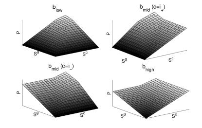
(a) Surface plots of blowsubscript𝑏lowb_{\text{low}}, bmidsubscript𝑏midb_{\text{mid}} and bhighsubscript𝑏highb_{\text{high}}
Refer to caption
(b) blowsubscript𝑏lowb_{\text{low}}, bmidsubscript𝑏midb_{\text{mid}}, bhighsubscript𝑏highb_{\text{high}} for fixed Scsuperscript𝑆𝑐S^{c} (ξ¯c>ξ¯gsuperscript¯𝜉𝑐superscript¯𝜉𝑔\bar{\xi}^{c}>\bar{\xi}^{g}).
Figure 3. Illustration of the dependence of power spot price on fuel prices and demand

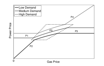
Figure 3 illustrates the dependence of the power price on the input factors, namely the prices of coal and gas and the demand for electricity. For the purpose of these plots we assumed throughout that ξ¯c>ξ¯gsuperscript¯𝜉𝑐superscript¯𝜉𝑔\bar{\xi}^{c}>\bar{\xi}^{g}. The surfaces in Figure 3a represent the functions blowsubscript𝑏lowb_{\text{low}}, bmidsubscript𝑏midb_{\text{mid}} and bhighsubscript𝑏highb_{\text{high}} for demand fixed in the corresponding intervals. In Figure 3b we aggregate the information contained in Figure 3a for a fixed coal price; i.e. we compare the dependency of the electricity price on the gas price for each of the three relevant demand levels. In all three cases electricity is non-decreasing in fuel price and is constant against Stisubscriptsuperscript𝑆𝑖𝑡S^{i}_{t} if fuel i𝑖i is not at the margin (i.e., iM𝑖𝑀i\notin M). Furthermore, in each case Ptsubscript𝑃𝑡P_{t} is linear in the sole marginal fuel for sufficiently low or high gas price, and non-linear in both fuels in the quadrilateral in the middle. This characterises the region of coal-gas overlap, where both technologies jointly set the price. Finally, note that labels P1 to P5 indicate regions corresponding to rows one to five of Table 1.

3.3. Extension to Capture Spikes and Negative Prices

In this section we suggest a simple extension of the bid stack model in order to more accurately capture the spot price density in markets that are prone to dramatic price spikes during peak hours or sudden negative prices at off-peak times. Importantly, this modification does not impact the availability of closed-form solutions for forwards or spread options, which we introduce in §4 and §5.

Let (Xt)subscript𝑋𝑡(X_{t}) be a stochastic process adpated to the filtration t0superscriptsubscript𝑡0\mathcal{F}_{t}^{0}, as is Dtsubscript𝐷𝑡D_{t}. Further, we assume that the relationship between the two processes satisfies

{Xt0}={ωΩ:Dt=0}and{Xt0}={Dt=ξ¯}.formulae-sequencesubscript𝑋𝑡0conditional-set𝜔Ωsubscript𝐷𝑡0andsubscript𝑋𝑡0subscript𝐷𝑡¯𝜉\{X_{t}\leq 0\}=\{\omega\in\Omega:D_{t}=0\}\quad\text{and}\quad\{X_{t}\geq 0\}=\left\{D_{t}=\bar{\xi}\right\}.

The difference between (Dt)subscript𝐷𝑡(D_{t}) and (Xt)subscript𝑋𝑡(X_{t}) is that (Dt)subscript𝐷𝑡(D_{t}) is restricted to take values in [0,ξ¯]0¯𝜉[0,\bar{\xi}] only, whereas the process (Xt)subscript𝑋𝑡(X_{t}) can potentially take values on the entire real line.

In the event that demand hits zero or ξ¯¯𝜉\bar{\xi}, we say that the market is in a negative price regime (for which negative prices are possible, but not guaranteed) or a spike regime and we redefine the electricity price at these points to be given respectively by

bn(x,𝐬)subscript𝑏𝑛𝑥𝐬\displaystyle b_{n}\left(x,\mathbf{s}\right) :=b(0,𝐬)exp(mnx)+1,assignabsent𝑏0𝐬subscript𝑚𝑛𝑥1\displaystyle:=b(0,\mathbf{s})-\exp(-m_{n}x)+1, for (x,𝐬)(,0]×+2,for 𝑥𝐬0superscriptsubscript2\displaystyle\text{for }(x,\mathbf{s})\in(-\infty,0]\times\mathbb{R}_{+}^{2},
andbs(x,𝐬)andsubscript𝑏𝑠𝑥𝐬\displaystyle\text{and}\quad b_{s}\left(x,\mathbf{s}\right) :=b(ξ¯,𝐬)+exp(ms(xξ¯))1,assignabsent𝑏¯𝜉𝐬subscript𝑚𝑠𝑥¯𝜉1\displaystyle:=b\left(\bar{\xi},\mathbf{s}\right)+\exp\left(m_{s}\left(x-\bar{\xi}\right)\right)-1, for (x,𝐬)[ξ¯,)×+2.for 𝑥𝐬¯𝜉superscriptsubscript2\displaystyle\text{for }(x,\mathbf{s})\in\left[\bar{\xi},\infty\right)\times\mathbb{R}_{+}^{2}.

Under this extension, the power price expression from Corollary 2 is therefore replaced by

P^t:=bn(Xt,𝐒t)𝕀{0}(Dt)+blow(Dt,𝐒t)𝕀(0,ξ¯i](Dt)+bmid(Dt,𝐒t)𝕀(ξ¯i,ξ¯j](Dt)+bhigh(Dt,𝐒t)𝕀(ξ¯j,ξ¯)(Dt)+bs(Xt,𝐒t)𝕀{ξ¯}(Dt),assignsubscript^𝑃𝑡subscript𝑏𝑛subscript𝑋𝑡subscript𝐒𝑡subscript𝕀0subscript𝐷𝑡subscript𝑏lowsubscript𝐷𝑡subscript𝐒𝑡subscript𝕀0superscript¯𝜉𝑖subscript𝐷𝑡subscript𝑏midsubscript𝐷𝑡subscript𝐒𝑡subscript𝕀superscript¯𝜉𝑖superscript¯𝜉𝑗subscript𝐷𝑡subscript𝑏highsubscript𝐷𝑡subscript𝐒𝑡subscript𝕀superscript¯𝜉𝑗¯𝜉subscript𝐷𝑡subscript𝑏𝑠subscript𝑋𝑡subscript𝐒𝑡subscript𝕀¯𝜉subscript𝐷𝑡\hat{P}_{t}:=b_{n}\left(X_{t},\mathbf{S}_{t}\right)\mathbb{I}_{\{0\}}(D_{t})+b_{\text{low}}\left(D_{t},\mathbf{S}_{t}\right)\mathbb{I}_{\left(0,\bar{\xi}^{i}\right]}(D_{t})\\ +b_{\text{mid}}\left(D_{t},\mathbf{S}_{t}\right)\mathbb{I}_{\left(\bar{\xi}^{i},\bar{\xi}^{j}\right]}(D_{t})+b_{\text{high}}\left(D_{t},\mathbf{S}_{t}\right)\mathbb{I}_{\left(\bar{\xi}^{j},\bar{\xi}\right)}(D_{t})+b_{s}\left(X_{t},\mathbf{S}_{t}\right)\mathbb{I}_{\left\{\bar{\xi}\right\}}(D_{t}),

where blowsubscript𝑏lowb_{\text{low}}, bmidsubscript𝑏midb_{\text{mid}}, bhighsubscript𝑏highb_{\text{high}} are defined in Corollary 2.

Note that the constants mn,ms>0subscript𝑚𝑛subscript𝑚𝑠0m_{n},m_{s}>0 determine how volatile prices are in these two regimes. In such cases, the price of electricity may now be interpreted as being set by a thin tail of miscellaneous bids, which correspond to no particular technology. Therefore, the difference between the electricity price implied by the bid stack and that defined by the negative price or spike regime is independent of fuel prices.

Remark 2.

It is possible to generate realistic spikes even in the base model (without the inclusion of the spike regime), simply by choosing one of the exponential fuel bid curves to be very steep (large misubscript𝑚𝑖m_{i}). However, this would come at the expense of realistically capturing changes in the merit order, as it artificially stretches the bids associated with that technology.

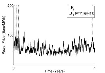
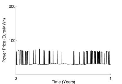
Figure 4 displays the electricity price through time as generated by the stack model for three different choices of parameters, for the same scenario. In Figure 4b we show a typical price path in the case that mcsubscript𝑚𝑐m_{c}, mgsubscript𝑚𝑔m_{g}, mssubscript𝑚𝑠m_{s} and mnsubscript𝑚𝑛m_{n} are very small. This corresponds to a step function bid stack and has been suggested by Aid et al [1]. Clearly, the prices do not exhibit enough variation to match observed time series. The solid line in Figure 4a corresponds to more realistic values of mcsubscript𝑚𝑐m_{c} and mgsubscript𝑚𝑔m_{g}; the dashed line illustrates the modification of this path due to the choice of larger values for mssubscript𝑚𝑠m_{s} and mnsubscript𝑚𝑛m_{n}. Both paths capture the stylized facts of electricity price time series reasonably well. For the purpose of this simulation the prices of coal and gas have been modeled as exponential Ornstein-Uhlenbeck (OU) processes, and demand as an OU process with seasonality truncated at zero and ξ¯¯𝜉\bar{\xi} (with (Xt)subscript𝑋𝑡(X_{t}) its untruncated version). However, the choice of model for these factors is secondary at this stage, as we are emphasizing the consequences of our choice for the bid stack itself.
Refer to caption
(a) Ptsubscript𝑃𝑡P_{t} and P^tsubscript^𝑃𝑡\hat{P}_{t} with mc,mg>0subscript𝑚𝑐subscript𝑚𝑔0m_{c},m_{g}>0.
Refer to caption
(b) Ptsubscript𝑃𝑡P_{t} with mc,mgsubscript𝑚𝑐subscript𝑚𝑔m_{c},m_{g} small.
Figure 4. Simulation of the power price for typical parameters

4. Forward Contracts

We now turn to the analysis of forward contracts in our structural framework. For the sake of simplicity, we ignore delivery periods and suggest that T𝑇T be considered as a representative date in a typical monthly delivery period (see [4] for more on handling delivery periods). For the purpose of the present discussion, a forward contract with maturity T𝑇T is defined by the payoff

PTFtp,subscript𝑃𝑇superscriptsubscript𝐹𝑡𝑝P_{T}-F_{t}^{p},

where Ftpsuperscriptsubscript𝐹𝑡𝑝F_{t}^{p} is the delivery price agreed at the initial date t𝑡t, and paid by the holder of the long position at T𝑇T. Simple arbitrage arguments (cf. [26]) imply that

Ftp=𝔼[PT|t].superscriptsubscript𝐹𝑡𝑝superscript𝔼delimited-[]conditionalsubscript𝑃𝑇subscript𝑡F_{t}^{p}=\mathbb{E}^{\mathbb{Q}}\left[P_{T}|\mathcal{F}_{t}\right].

The result of Corollary 2 shows that the payoff of the forward is a function of demand and fuels, so that the electricity forward contract becomes a derivative on fuel prices and demand.

4.1. Closed Form Forward Prices

For the explicit calculation of forward prices the following property of Gaussian densities will be useful (see [21] for an application of this result to pricing compound options). Let φ1subscript𝜑1\varphi_{1} denote the density of the standard univariate Gaussian distribution, and Φ1()subscriptΦ1\Phi_{1}(\cdot) and Φ2(,;ρ)subscriptΦ2𝜌\Phi_{2}(\cdot,\cdot;\rho) the cumulative distribution functions (cdfs) of the univariate and bivariate (correlation ρ𝜌\rho) standard Gaussian distributions respectively.

Lemma 1.

The following relationship holds between φ1subscript𝜑1\varphi_{1}, Φ1subscriptΦ1\Phi_{1} and Φ2subscriptΦ2\Phi_{2}:

(8) aexp(l1+q1x)φ1(x)Φ1(l2+q2x)dx=exp(l1+q122)Φ2(aq1,l2+q1q21+q22;q21+q22),superscriptsubscript𝑎subscript𝑙1subscript𝑞1𝑥subscript𝜑1𝑥subscriptΦ1subscript𝑙2subscript𝑞2𝑥differential-d𝑥subscript𝑙1superscriptsubscript𝑞122subscriptΦ2𝑎subscript𝑞1subscript𝑙2subscript𝑞1subscript𝑞21superscriptsubscript𝑞22subscript𝑞21superscriptsubscript𝑞22\int_{-\infty}^{a}\exp\left(l_{1}+q_{1}x\right)\varphi_{1}(x)\Phi_{1}(l_{2}+q_{2}x)\ \mathrm{d}x=\exp\left(l_{1}+\frac{q_{1}^{2}}{2}\right)\Phi_{2}\left(a-q_{1},\frac{l_{2}+q_{1}q_{2}}{\sqrt{1+q_{2}^{2}}};\frac{-q_{2}}{\sqrt{1+q_{2}^{2}}}\right),

for all l1,l2,q1,q2subscript𝑙1subscript𝑙2subscript𝑞1subscript𝑞2l_{1},l_{2},q_{1},q_{2}\in\mathbb{R} and a{}𝑎a\in\mathbb{R}\cup\{\infty\}.

Proof.

In equation (8) combine the explicit exponential term with the one contained in φ1subscript𝜑1\varphi_{1} and complete the square. Then, define the change of variable (x,y)(z,w)𝑥𝑦𝑧𝑤(x,y)\to(z,w) by

x=z+q1,y=w1+q22+q2(xq1).formulae-sequence𝑥𝑧subscript𝑞1𝑦𝑤1superscriptsubscript𝑞22subscript𝑞2𝑥subscript𝑞1x=z+q_{1},\quad y=w\sqrt{1+q_{2}^{2}}+q_{2}(x-q_{1}).

The determinant of the Jacobian matrix J𝐽J associated with this transformation is |J|=1+q22𝐽1superscriptsubscript𝑞22|J|=\sqrt{1+q_{2}^{2}}. Performing the change of variable leads to the right hand side of (8). ∎

For the main result in this section we denote by Ftisubscriptsuperscript𝐹𝑖𝑡F^{i}_{t}, iI𝑖𝐼i\in I, the delivery price of a forward contract on fuel i𝑖i with maturity T𝑇T and write 𝐅t:=(Ftc,Ftc)assignsubscript𝐅𝑡subscriptsuperscript𝐹𝑐𝑡subscriptsuperscript𝐹𝑐𝑡\mathbf{F}_{t}:=(F^{c}_{t},F^{c}_{t}).

Proposition 2.

Given I={c,g}𝐼𝑐𝑔I=\{c,g\}, if under \mathbb{Q}, the random variables log(STc)subscriptsuperscript𝑆𝑐𝑇\log(S^{c}_{T}) and log(STg)subscriptsuperscript𝑆𝑔𝑇\log(S^{g}_{T}) are jointly Gaussian with means μcsubscript𝜇𝑐\mu_{c} and μgsubscript𝜇𝑔\mu_{g}, variances σc2superscriptsubscript𝜎𝑐2\sigma_{c}^{2} and σg2superscriptsubscript𝜎𝑔2\sigma_{g}^{2} and correlation ρ𝜌\rho, and if the demand DTsubscript𝐷𝑇D_{T} at maturity is independent of TWsubscriptsuperscript𝑊𝑇\mathcal{F}^{W}_{T}, then for t[0,T]𝑡0𝑇t\in[0,T], the delivery price of a forward contract on electricity is given by:

(9) Ftp=0ξ¯iflow(D,𝐅t)ϕd(D)dD+ξ¯iξ¯i+fmid(D,𝐅t)ϕd(D)dD+ξ¯i+ξ¯fhigh(D,𝐅t)ϕd(D)dD,superscriptsubscript𝐹𝑡𝑝superscriptsubscript0superscript¯𝜉subscript𝑖subscript𝑓low𝐷subscript𝐅𝑡subscriptitalic-ϕ𝑑𝐷differential-d𝐷superscriptsubscriptsuperscript¯𝜉subscript𝑖superscript¯𝜉subscript𝑖subscript𝑓mid𝐷subscript𝐅𝑡subscriptitalic-ϕ𝑑𝐷differential-d𝐷superscriptsubscriptsuperscript¯𝜉subscript𝑖¯𝜉subscript𝑓high𝐷subscript𝐅𝑡subscriptitalic-ϕ𝑑𝐷differential-d𝐷F_{t}^{p}=\int_{0}^{\bar{\xi}^{i_{-}}}f_{\text{low}}\left(D,\mathbf{F}_{t}\right)\phi_{d}(D)\ \mathrm{d}D+\int_{\bar{\xi}^{i_{-}}}^{\bar{\xi}^{i_{+}}}f_{\text{mid}}\left(D,\mathbf{F}_{t}\right)\phi_{d}(D)\ \mathrm{d}D+\int_{\bar{\xi}^{i_{+}}}^{\bar{\xi}}f_{\text{high}}\left(D,\mathbf{F}_{t}\right)\phi_{d}(D)\ \mathrm{d}D,

where ϕdsubscriptitalic-ϕ𝑑\phi_{d} denotes the density of the random variable DTsubscript𝐷𝑇D_{T} and, for (ξ,𝐱)[0,ξ¯]×+2𝜉𝐱0¯𝜉superscriptsubscript2(\xi,\mathbf{x})\in[0,\bar{\xi}]\times\mathbb{R}_{+}^{2}:

flow(ξ,𝐱)=iIbi(ξ,xi)Φ1(Ri(ξ,0)/σ)+bcg(ξ,𝐱)exp(αcαgσ2/2)[1iIΦ1(Ri(ξ,0)/σ+αjσ)],subscript𝑓low𝜉𝐱subscript𝑖𝐼subscript𝑏𝑖𝜉superscript𝑥𝑖subscriptΦ1subscript𝑅𝑖𝜉0𝜎subscript𝑏𝑐𝑔𝜉𝐱subscript𝛼𝑐subscript𝛼𝑔superscript𝜎22delimited-[]1subscript𝑖𝐼subscriptΦ1subscript𝑅𝑖𝜉0𝜎subscript𝛼𝑗𝜎f_{\text{low}}\left(\xi,\mathbf{x}\right)=\sum_{i\in I}b_{i}\left(\xi,x^{i}\right)\Phi_{1}\left(R_{i}(\xi,0)/\sigma\right)\\ +b_{cg}(\xi,\mathbf{x})\exp\left(-\alpha_{c}\alpha_{g}\sigma^{2}/2\right)\left[1-\sum_{i\in I}\Phi_{1}\left(R_{i}(\xi,0)/\sigma+\alpha_{j}\sigma\right)\right],
fmid(ξ,𝐱)=bi+(ξξ¯i,xi+)Φ1(Ri+(ξξ¯i,ξ¯i)/σ)+bi+(ξ,xi+)Φ1(Ri+(ξ,0)/σ)+bcg(ξ,𝐱)exp(αcαgσ2/2)[Φ1(Ri+(ξξ¯i,ξ¯i)/σ+αiσ)Φ1(Ri+(ξ,0)/σ+αiσ)],subscript𝑓mid𝜉𝐱subscript𝑏subscript𝑖𝜉superscript¯𝜉subscript𝑖superscript𝑥subscript𝑖subscriptΦ1subscript𝑅subscript𝑖𝜉superscript¯𝜉subscript𝑖superscript¯𝜉subscript𝑖𝜎subscript𝑏subscript𝑖𝜉superscript𝑥subscript𝑖subscriptΦ1subscript𝑅subscript𝑖𝜉0𝜎subscript𝑏𝑐𝑔𝜉𝐱subscript𝛼𝑐subscript𝛼𝑔superscript𝜎22delimited-[]subscriptΦ1subscript𝑅subscript𝑖𝜉superscript¯𝜉subscript𝑖superscript¯𝜉subscript𝑖𝜎subscript𝛼subscript𝑖𝜎subscriptΦ1subscript𝑅subscript𝑖𝜉0𝜎subscript𝛼subscript𝑖𝜎f_{\text{mid}}\left(\xi,\mathbf{x}\right)=b_{i_{+}}\left(\xi-\bar{\xi}^{i_{-}},x^{i_{+}}\right)\Phi_{1}\left(-R_{i_{+}}\left(\xi-\bar{\xi}^{i_{-}},\bar{\xi}^{i_{-}}\right)/\sigma\right)+b_{i_{+}}\left(\xi,x^{i_{+}}\right)\Phi_{1}\left(R_{i_{+}}(\xi,0)/\sigma\right)\\ +b_{cg}(\xi,\mathbf{x})\exp\left(-\alpha_{c}\alpha_{g}\sigma^{2}/2\right)\left[\Phi_{1}\left(R_{i_{+}}\left(\xi-\bar{\xi}^{i_{-}},\bar{\xi}^{i_{-}}\right)/\sigma+\alpha_{i_{-}}\sigma\right)-\Phi_{1}\left(R_{i_{+}}\left(\xi,0\right)/\sigma+\alpha_{i_{-}}\sigma\right)\right],
fhigh(ξ,𝐱)=iIbi(ξξ¯j,xi)Φ1(Ri(ξξ¯j,ξ¯j)/σ)+bcg(ξ,𝐱)exp(αcαgσ2/2)[1+iIΦ1(Ri(ξξ¯j,ξ¯j)/σ+αjσ)],subscript𝑓high𝜉𝐱subscript𝑖𝐼subscript𝑏𝑖𝜉superscript¯𝜉𝑗superscript𝑥𝑖subscriptΦ1subscript𝑅𝑖𝜉superscript¯𝜉𝑗superscript¯𝜉𝑗𝜎subscript𝑏𝑐𝑔𝜉𝐱subscript𝛼𝑐subscript𝛼𝑔superscript𝜎22delimited-[]1subscript𝑖𝐼subscriptΦ1subscript𝑅𝑖𝜉superscript¯𝜉𝑗superscript¯𝜉𝑗𝜎subscript𝛼𝑗𝜎f_{\text{high}}\left(\xi,\mathbf{x}\right)=\sum_{i\in I}b_{i}\left(\xi-\bar{\xi}^{j},x^{i}\right)\Phi_{1}\left(-R_{i}\left(\xi-\bar{\xi}^{j},\bar{\xi}^{j}\right)/\sigma\right)\\ +b_{cg}(\xi,\mathbf{x})\exp\left(-\alpha_{c}\alpha_{g}\sigma^{2}/2\right)\left[-1+\sum_{i\in I}\Phi_{1}\left(R_{i}\left(\xi-\bar{\xi}^{j},\bar{\xi}^{j}\right)/\sigma+\alpha_{j}\sigma\right)\right],

where j=I{i}𝑗𝐼𝑖j=I\setminus\{i\}, the constants αc,αg,β,γsubscript𝛼𝑐subscript𝛼𝑔𝛽𝛾\alpha_{c},\alpha_{g},\beta,\gamma are as defined in Corollary 2, and

σ2superscript𝜎2\displaystyle\sigma^{2} :=σc22ρσcσg+σg2,assignabsentsuperscriptsubscript𝜎𝑐22𝜌subscript𝜎𝑐subscript𝜎𝑔superscriptsubscript𝜎𝑔2\displaystyle:=\sigma_{c}^{2}-2\rho\sigma_{c}\sigma_{g}+\sigma_{g}^{2},
Ri(ξi,ξj)subscript𝑅𝑖subscript𝜉𝑖subscript𝜉𝑗\displaystyle R_{i}\left(\xi_{i},\xi_{j}\right) :=kj+mjξjkimiξi+log(Ftj)log(Fti)12σ2.assignabsentsubscript𝑘𝑗subscript𝑚𝑗subscript𝜉𝑗subscript𝑘𝑖subscript𝑚𝑖subscript𝜉𝑖subscriptsuperscript𝐹𝑗𝑡subscriptsuperscript𝐹𝑖𝑡12superscript𝜎2\displaystyle:=k_{j}+m_{j}\xi_{j}-k_{i}-m_{i}\xi_{i}+\log\left(F^{j}_{t}\right)-\log\left(F^{i}_{t}\right)-\frac{1}{2}\sigma^{2}.
Proof.

By iterated conditioning, for t[0,T]𝑡0𝑇t\in[0,T], the price of the electricity forward Ftpsuperscriptsubscript𝐹𝑡𝑝F_{t}^{p} is given by

(10) Ftp:=𝔼[PT|t]=𝔼[𝔼[b(DT,𝐒T)|T0tW]|t].assignsuperscriptsubscript𝐹𝑡𝑝superscript𝔼delimited-[]conditionalsubscript𝑃𝑇subscript𝑡superscript𝔼delimited-[]conditionalsuperscript𝔼delimited-[]conditional𝑏subscript𝐷𝑇subscript𝐒𝑇subscriptsuperscript0𝑇subscriptsuperscript𝑊𝑡subscript𝑡F_{t}^{p}:=\mathbb{E}^{\mathbb{Q}}\left[\left.P_{T}\right|\mathcal{F}_{t}\right]=\mathbb{E}^{\mathbb{Q}}\left.\left[\left.\mathbb{E}^{\mathbb{Q}}\left[b(D_{T},\mathbf{S}_{T})\right|\mathcal{F}^{0}_{T}\vee\mathcal{F}^{W}_{t}\right]\right|\mathcal{F}_{t}\right].

The outer expectation can be written as the sum of three integrals corresponding to the cases DT[0,ξ¯i]subscript𝐷𝑇0superscript¯𝜉subscript𝑖D_{T}\in[0,\bar{\xi}^{i_{-}}], DT[ξ¯i,ξ¯i+]subscript𝐷𝑇superscript¯𝜉subscript𝑖superscript¯𝜉subscript𝑖D_{T}\in[\bar{\xi}^{i_{-}},\bar{\xi}^{i_{+}}] and DT[ξ¯i+,0]subscript𝐷𝑇superscript¯𝜉subscript𝑖0D_{T}\in[\bar{\xi}^{i_{+}},0] respectively. We consider the first case and derive the flowsubscript𝑓lowf_{\text{low}} term. The other cases corresponding to fmidsubscript𝑓midf_{\text{mid}} and fhighsubscript𝑓highf_{\text{high}} are proven similarly.

From Corollary 2 we know that b=blow𝑏subscript𝑏lowb=b_{\text{low}} for DT[0,ξ¯i]subscript𝐷𝑇0superscript¯𝜉subscript𝑖D_{T}\in[0,\bar{\xi}^{i_{-}}]. This expression for PTsubscript𝑃𝑇P_{T} is easily written in terms of independent standard Gaussian variables 𝐙:=(Z1,Z2)assign𝐙subscript𝑍1subscript𝑍2\mathbf{Z}:=(Z_{1},Z_{2}) by using the identity

(log(STc)log(STg))=(μcμg)+(σc2ρσcσgρσcσgσg2)(Z1Z2).subscriptsuperscript𝑆𝑐𝑇subscriptsuperscript𝑆𝑔𝑇subscript𝜇𝑐subscript𝜇𝑔superscriptsubscript𝜎𝑐2𝜌subscript𝜎𝑐subscript𝜎𝑔𝜌subscript𝜎𝑐subscript𝜎𝑔superscriptsubscript𝜎𝑔2subscript𝑍1subscript𝑍2\left(\begin{array}[]{c}\log\left(S^{c}_{T}\right)\\ \log\left(S^{g}_{T}\right)\end{array}\right)=\left(\begin{array}[]{c}\mu_{c}\\ \mu_{g}\end{array}\right)+\left(\begin{array}[]{cc}\sigma_{c}^{2}&\rho\sigma_{c}\sigma_{g}\\ \rho\sigma_{c}\sigma_{g}&\sigma_{g}^{2}\end{array}\right)\left(\begin{array}[]{c}Z_{1}\\ Z_{2}\end{array}\right).

Defining d^:=𝔼[DT|T0]assign^𝑑superscript𝔼delimited-[]conditionalsubscript𝐷𝑇subscriptsuperscript0𝑇\hat{d}:=\mathbb{E}^{\mathbb{Q}}[D_{T}|\mathcal{F}^{0}_{T}], the inner expectation can now be written in integral form as

𝔼[b~low(d^,𝐙)]=Ic+Ig+Icg,𝔼delimited-[]subscript~𝑏low^𝑑𝐙subscript𝐼𝑐subscript𝐼𝑔subscript𝐼𝑐𝑔\mathbb{E}\left[\tilde{b}_{\text{low}}\left(\hat{d},\mathbf{Z}\right)\right]=I_{c}+I_{g}+I_{cg},

where b~low(ξ,𝐙):=blow(ξ,𝐒)assignsubscript~𝑏low𝜉𝐙subscript𝑏low𝜉𝐒\tilde{b}_{\text{low}}(\xi,\mathbf{Z}):=b_{\text{low}}(\xi,\mathbf{S}) and the expectation is computed with respect to the law of 𝐙𝐙\mathbf{Z}. For example, after completing the square in z1subscript𝑧1z_{1},

Ic=exp(l1+q1z2)ϕ1(z2)Φ1(l2+q2z2)dz2,subscript𝐼𝑐superscriptsubscriptsubscript𝑙1subscript𝑞1subscript𝑧2subscriptitalic-ϕ1subscript𝑧2subscriptΦ1subscript𝑙2subscript𝑞2subscript𝑧2differential-dsubscript𝑧2I_{c}=\int_{-\infty}^{\infty}\exp\left(l_{1}+q_{1}z_{2}\right)\phi_{1}(z_{2})\Phi_{1}(l_{2}+q_{2}z_{2})\ \mathrm{d}z_{2},

with

l1subscript𝑙1\displaystyle l_{1} :=μc+kc+mcd^+σc42,assignabsentsubscript𝜇𝑐subscript𝑘𝑐subscript𝑚𝑐^𝑑superscriptsubscript𝜎𝑐42\displaystyle:=\mu_{c}+k_{c}+m_{c}\hat{d}+\frac{\sigma_{c}^{4}}{2}, l2::subscript𝑙2absent\displaystyle l_{2}: =σc2μc+kc+mcd^+μgσc(σcρσg),absentsuperscriptsubscript𝜎𝑐2subscript𝜇𝑐subscript𝑘𝑐subscript𝑚𝑐^𝑑subscript𝜇𝑔subscript𝜎𝑐subscript𝜎𝑐𝜌subscript𝜎𝑔\displaystyle=-\sigma_{c}^{2}-\frac{\mu_{c}+k_{c}+m_{c}\hat{d}+\mu_{g}}{\sigma_{c}(\sigma_{c}-\rho\sigma_{g})},
q1subscript𝑞1\displaystyle q_{1} :=ρσcσg,assignabsent𝜌subscript𝜎𝑐subscript𝜎𝑔\displaystyle:=\rho\sigma_{c}\sigma_{g}, q2subscript𝑞2\displaystyle q_{2} :=σg(σgρσc)σc(σcρσg).assignabsentsubscript𝜎𝑔subscript𝜎𝑔𝜌subscript𝜎𝑐subscript𝜎𝑐subscript𝜎𝑐𝜌subscript𝜎𝑔\displaystyle:=\frac{\sigma_{g}(\sigma_{g}-\rho\sigma_{c})}{\sigma_{c}(\sigma_{c}-\rho\sigma_{g})}.

Lemma 1 now applies with a=𝑎a=\infty. Igsubscript𝐼𝑔I_{g} and Icgsubscript𝐼𝑐𝑔I_{cg} are computed similarly. In all terms, we substitute for μisubscript𝜇𝑖\mu_{i} using the following standard result. For iI𝑖𝐼i\in I,

(11) Fti=𝔼[STi|t]=exp(μi+12σi2), for t[0,T].formulae-sequencesubscriptsuperscript𝐹𝑖𝑡superscript𝔼delimited-[]conditionalsubscriptsuperscript𝑆𝑖𝑇subscript𝑡subscript𝜇𝑖12superscriptsubscript𝜎𝑖2 for 𝑡0𝑇F^{i}_{t}=\mathbb{E}^{\mathbb{Q}}\left[\left.S^{i}_{T}\right|\mathcal{F}_{t}\right]=\exp\left(\mu_{i}+\frac{1}{2}\sigma_{i}^{2}\right),\quad\text{ for }t\in[0,T].

Substituting the resulting expression for the inner expectation into the outer expectation in (10) yields the first term in the proposition. ∎

Remark 3.

The assumption of lognormal fuel prices in Proposition 2 is a very common and natural choice for modeling energy (non-power) prices. Geometric Brownian Motion (GBM) with constant convenience yield, the classical exponential OU model of Schwartz [28], and the two-factor version of Schwartz and Smith [29] all satisfy the lognormality assumption.

The above result does not depend upon any assumption on the distribution of the demand at maturity, and as a result, it can easily be computed numerically for any distribution. In markets where reasonably reliable load forecasts exist, one may consider demand to be a deterministic function, in which case the integrals in (9) are not needed and the forward price becomes explicit. For cases when load forecasts are not reliable, we introduce another convenient special case below, where demand at maturity has a Gaussian distribution truncated at zero and ξ¯¯𝜉\bar{\xi}.

To simplify and shorten the notation we introduce the following shorthand notation:

Φ22×1([x1x2],y;ρ):=Φ2(x1,y;ρ)Φ2(x2,y;ρ).assignsuperscriptsubscriptΦ221delimited-[]subscript𝑥1subscript𝑥2𝑦𝜌subscriptΦ2subscript𝑥1𝑦𝜌subscriptΦ2subscript𝑥2𝑦𝜌\Phi_{2}^{2\times 1}\left(\left[\begin{array}[]{c}x_{1}\\ x_{2}\end{array}\right],y;\rho\right):=\Phi_{2}(x_{1},y;\rho)-\Phi_{2}(x_{2},y;\rho).
Corollary 3.

In addition to the assumptions in Proposition 2 let demand at maturity satisfy

DT=max(0,min(ξ¯,XT)),subscript𝐷𝑇0¯𝜉subscript𝑋𝑇D_{T}=\max\left(0,\min\left(\bar{\xi},X_{T}\right)\right),

where XTN(μd,σd2)similar-tosubscript𝑋𝑇𝑁subscript𝜇𝑑superscriptsubscript𝜎𝑑2X_{T}\sim N(\mu_{d},\sigma_{d}^{2}) is independent of 𝐒Tsubscript𝐒𝑇\mathbf{S}_{T} under \mathbb{Q}. Then for t[0,T]𝑡0𝑇t\in[0,T], the delivery price of a forward contract is given explicitly by

Ftp=iIexp(mi2σd22){bi(μd,Fti)Φ22×1([ξ¯iμdσdmiσdμdσdmiσd],Ri(μd,0)mi2σd2σi,d;miσdσi,d)+bi(μdξ¯j,Fti)Φ22×1([ξ¯μdσdmiσdξ¯jμdσdmiσd],Ri(μdξ¯j,ξ¯j)+mi2σd2σi,d;miσdσi,d)}+iIδiexp(η)bcg(μd,𝐅t){Φ22×1([ξ¯iμdσdγσdμdσdγσd],Ri(μd,0)+αjσ2γmiσd2δiσi,d;miσdδiσi,d)+Φ22×1([ξ¯μdσdγσdξ¯jμdσdγσd],Ri(μdξ¯j,ξ¯j)+αjσ2γmiσd2δiσi,d;miσdδiσi,d)}+Φ1(μdσd)iIbi(0,Fti)Φ1(Ri(0,0)σ)+Φ1(μdξ¯σd)iIbi(ξ¯i,Fti)Φ1(Ri(ξ¯i,ξ¯j)σ),superscriptsubscript𝐹𝑡𝑝subscript𝑖𝐼superscriptsubscript𝑚𝑖2superscriptsubscript𝜎𝑑22subscript𝑏𝑖subscript𝜇𝑑superscriptsubscript𝐹𝑡𝑖superscriptsubscriptΦ221delimited-[]superscript¯𝜉𝑖subscript𝜇𝑑subscript𝜎𝑑subscript𝑚𝑖subscript𝜎𝑑subscript𝜇𝑑subscript𝜎𝑑subscript𝑚𝑖subscript𝜎𝑑subscript𝑅𝑖subscript𝜇𝑑0superscriptsubscript𝑚𝑖2superscriptsubscript𝜎𝑑2subscript𝜎𝑖𝑑subscript𝑚𝑖subscript𝜎𝑑subscript𝜎𝑖𝑑subscript𝑏𝑖subscript𝜇𝑑superscript¯𝜉𝑗subscriptsuperscript𝐹𝑖𝑡superscriptsubscriptΦ221delimited-[]¯𝜉subscript𝜇𝑑subscript𝜎𝑑subscript𝑚𝑖subscript𝜎𝑑superscript¯𝜉𝑗subscript𝜇𝑑subscript𝜎𝑑subscript𝑚𝑖subscript𝜎𝑑subscript𝑅𝑖subscript𝜇𝑑superscript¯𝜉𝑗superscript¯𝜉𝑗superscriptsubscript𝑚𝑖2superscriptsubscript𝜎𝑑2subscript𝜎𝑖𝑑subscript𝑚𝑖subscript𝜎𝑑subscript𝜎𝑖𝑑subscript𝑖𝐼subscript𝛿𝑖𝜂subscript𝑏𝑐𝑔subscript𝜇𝑑subscript𝐅𝑡superscriptsubscriptΦ221delimited-[]superscript¯𝜉𝑖subscript𝜇𝑑subscript𝜎𝑑𝛾subscript𝜎𝑑subscript𝜇𝑑subscript𝜎𝑑𝛾subscript𝜎𝑑subscript𝑅𝑖subscript𝜇𝑑0subscript𝛼𝑗superscript𝜎2𝛾subscript𝑚𝑖superscriptsubscript𝜎𝑑2subscript𝛿𝑖subscript𝜎𝑖𝑑subscript𝑚𝑖subscript𝜎𝑑subscript𝛿𝑖subscript𝜎𝑖𝑑superscriptsubscriptΦ221delimited-[]¯𝜉subscript𝜇𝑑subscript𝜎𝑑𝛾subscript𝜎𝑑superscript¯𝜉𝑗subscript𝜇𝑑subscript𝜎𝑑𝛾subscript𝜎𝑑subscript𝑅𝑖subscript𝜇𝑑superscript¯𝜉𝑗superscript¯𝜉𝑗subscript𝛼𝑗superscript𝜎2𝛾subscript𝑚𝑖superscriptsubscript𝜎𝑑2subscript𝛿𝑖subscript𝜎𝑖𝑑subscript𝑚𝑖subscript𝜎𝑑subscript𝛿𝑖subscript𝜎𝑖𝑑subscriptΦ1subscript𝜇𝑑subscript𝜎𝑑subscript𝑖𝐼subscript𝑏𝑖0subscriptsuperscript𝐹𝑖𝑡subscriptΦ1subscript𝑅𝑖00𝜎subscriptΦ1subscript𝜇𝑑¯𝜉subscript𝜎𝑑subscript𝑖𝐼subscript𝑏𝑖superscript¯𝜉𝑖subscriptsuperscript𝐹𝑖𝑡subscriptΦ1subscript𝑅𝑖superscript¯𝜉𝑖superscript¯𝜉𝑗𝜎F_{t}^{p}=\sum_{i\in I}\exp\left(\frac{m_{i}^{2}\sigma_{d}^{2}}{2}\right)\left\{b_{i}\left(\mu_{d},F_{t}^{i}\right)\Phi_{2}^{2\times 1}\left(\left[\begin{array}[]{c}\frac{\bar{\xi}^{i}-\mu_{d}}{\sigma_{d}}-m_{i}\sigma_{d}\\ \frac{-\mu_{d}}{\sigma_{d}}-m_{i}\sigma_{d}\end{array}\right],\frac{R_{i}(\mu_{d},0)-m_{i}^{2}\sigma_{d}^{2}}{\sigma_{i,d}};\frac{m_{i}\sigma_{d}}{\sigma_{i,d}}\right)\right.\\ +\left.b_{i}\left(\mu_{d}-\bar{\xi}^{j},F^{i}_{t}\right)\Phi_{2}^{2\times 1}\left(\left[\begin{array}[]{c}\frac{\bar{\xi}-\mu_{d}}{\sigma_{d}}-m_{i}\sigma_{d}\\ \frac{\bar{\xi}^{j}-\mu_{d}}{\sigma_{d}}-m_{i}\sigma_{d}\end{array}\right],\frac{-R_{i}\left(\mu_{d}-\bar{\xi}^{j},\bar{\xi}^{j}\right)+m_{i}^{2}\sigma_{d}^{2}}{\sigma_{i,d}};\frac{-m_{i}\sigma_{d}}{\sigma_{i,d}}\right)\right\}\\ +\sum_{i\in I}\delta_{i}\exp\left(\eta\right)b_{cg}(\mu_{d},\mathbf{F}_{t})\left\{-\Phi_{2}^{2\times 1}\left(\left[\begin{array}[]{c}\frac{\bar{\xi}^{i}-\mu_{d}}{\sigma_{d}}-\gamma\sigma_{d}\\ \frac{-\mu_{d}}{\sigma_{d}}-\gamma\sigma_{d}\end{array}\right],\frac{R_{i}(\mu_{d},0)+\alpha_{j}\sigma^{2}-\gamma m_{i}\sigma_{d}^{2}}{\delta_{i}\sigma_{i,d}};\frac{m_{i}\sigma_{d}}{\delta_{i}\sigma_{i,d}}\right)\right.\\ +\left.\Phi_{2}^{2\times 1}\left(\left[\begin{array}[]{c}\frac{\bar{\xi}-\mu_{d}}{\sigma_{d}}-\gamma\sigma_{d}\\ \frac{\bar{\xi}^{j}-\mu_{d}}{\sigma_{d}}-\gamma\sigma_{d}\end{array}\right],\frac{R_{i}\left(\mu_{d}-\bar{\xi}^{j},\bar{\xi}^{j}\right)+\alpha_{j}\sigma^{2}-\gamma m_{i}\sigma_{d}^{2}}{\delta_{i}\sigma_{i,d}};\frac{m_{i}\sigma_{d}}{\delta_{i}\sigma_{i,d}}\right)\right\}\\ +\Phi_{1}\left(\frac{-\mu_{d}}{\sigma_{d}}\right)\sum_{i\in I}b_{i}\left(0,F^{i}_{t}\right)\Phi_{1}\left(\frac{R_{i}(0,0)}{\sigma}\right)+\Phi_{1}\left(\frac{\mu_{d}-\bar{\xi}}{\sigma_{d}}\right)\sum_{i\in I}b_{i}\left(\bar{\xi}^{i},F^{i}_{t}\right)\Phi_{1}\left(\frac{-R_{i}\left(\bar{\xi}^{i},\bar{\xi}^{j}\right)}{\sigma}\right),

where j=I{i}𝑗𝐼𝑖j=I\setminus\{i\}, δi=(1)𝕀{i=i+}subscript𝛿𝑖superscript1subscript𝕀𝑖subscript𝑖\delta_{i}=(-1)^{\mathbb{I}_{\{i=i_{+}\}}} and

σi,d2:=mi2σd2+σ2andη:=γ2σd2αcαgσ22.formulae-sequenceassignsuperscriptsubscript𝜎𝑖𝑑2superscriptsubscript𝑚𝑖2superscriptsubscript𝜎𝑑2superscript𝜎2andassign𝜂superscript𝛾2superscriptsubscript𝜎𝑑2subscript𝛼𝑐subscript𝛼𝑔superscript𝜎22\sigma_{i,d}^{2}:=m_{i}^{2}\sigma_{d}^{2}+\sigma^{2}\quad\text{and}\quad\eta:=\frac{\gamma^{2}\sigma_{d}^{2}-\alpha_{c}\alpha_{g}\sigma^{2}}{2}.
Proof.

We use Lemma 1 with a<𝑎a<\infty. After integrating over demand, each of the terms in flowsubscript𝑓lowf_{\text{low}}, fmidsubscript𝑓midf_{\text{mid}} and fhighsubscript𝑓highf_{\text{high}} turns into the difference between two bivariate Gaussian distribution functions. Simplifying the resulting terms leads to the result. ∎

Although the expression in Corollary 3 may appear quite involved, each of the terms can be readily identified with one of the five cases listed in Table 1, along with four terms (the last line of Ftpsuperscriptsubscript𝐹𝑡𝑝F_{t}^{p}) corresponding to the endpoints of the stack. Furthermore, it is noteworthy that as compared to Corollary 2, the fuel forward prices now replace the fuel spot prices in the bid stack curves bisubscript𝑏𝑖b_{i}, while μdsubscript𝜇𝑑\mu_{d} replaces demand. The Gaussian cdfs essentially weight these terms according to the probability of the various bid stack permutations. Thus Ftpsuperscriptsubscript𝐹𝑡𝑝F_{t}^{p} can become asymptotically linear in Ftcsuperscriptsubscript𝐹𝑡𝑐F_{t}^{c} or Ftgsuperscriptsubscript𝐹𝑡𝑔F_{t}^{g} when the probability of a single fuel being marginal goes to one. Finally, we note that a very similar closed-form expression is available for higher moments of PTsubscript𝑃𝑇P_{T} and given in Appendix A. Convenient expressions can also be found for covariances with fuels and for the Greeks (sensitivities with respect to underlying factors or parameters), but are not included.

Remark 4.

Under the extended model introduced in §3.3 to capture spikes, forward prices are given by the same expression as in Proposition 3 plus the following simple terms

exp(ms(μdξ¯)+12ms2σd2)Φ1(μdξ¯σd+msσd)Φ1(μdξ¯σd)exp(mnμd+12mn2σd2)Φ1(mnσdμdσd)+Φ1(μdσd)subscript𝑚𝑠subscript𝜇𝑑¯𝜉12superscriptsubscript𝑚𝑠2superscriptsubscript𝜎𝑑2subscriptΦ1subscript𝜇𝑑¯𝜉subscript𝜎𝑑subscript𝑚𝑠subscript𝜎𝑑subscriptΦ1subscript𝜇𝑑¯𝜉subscript𝜎𝑑subscript𝑚𝑛subscript𝜇𝑑12superscriptsubscript𝑚𝑛2superscriptsubscript𝜎𝑑2subscriptΦ1subscript𝑚𝑛subscript𝜎𝑑subscript𝜇𝑑subscript𝜎𝑑subscriptΦ1subscript𝜇𝑑subscript𝜎𝑑\exp\left(m_{s}(\mu_{d}-\bar{\xi})+\frac{1}{2}m_{s}^{2}\sigma_{d}^{2}\right)\Phi_{1}\left(\frac{\mu_{d}-\bar{\xi}}{\sigma_{d}}+m_{s}\sigma_{d}\right)-\Phi_{1}\left(\frac{\mu_{d}-\bar{\xi}}{\sigma_{d}}\right)\\ -\exp\left(-m_{n}\mu_{d}+\frac{1}{2}m_{n}^{2}\sigma_{d}^{2}\right)\Phi_{1}\left(m_{n}\sigma_{d}-\frac{\mu_{d}}{\sigma_{d}}\right)+\Phi_{1}\left(\frac{-\mu_{d}}{\sigma_{d}}\right)
Remark 5.

In most electricity markets, available capacity is often uncertain, due for example to the risk of generator outages. Since ξ¯isuperscript¯𝜉𝑖\bar{\xi}^{i} enters linearly in the exponential function in (6) like demand, an extension to stochastic capacity levels should be feasible, though rather involved. However, if capacity shocks are similar for both fuel types, this additional randomness could more easily be accounted for by adjusting demand parameters μdsubscript𝜇𝑑\mu_{d} and σdsubscript𝜎𝑑\sigma_{d}. More generally, we note that these parameters could in practice be chosen to calibrate the model to observed power forward (or option) prices, thus using the random variable DTsubscript𝐷𝑇D_{T} as a proxy for demand, capacity, and all other non fuel-related risk, along with corresponding risk premia.

4.2. Correlation Between Electricity and Fuel Forwards

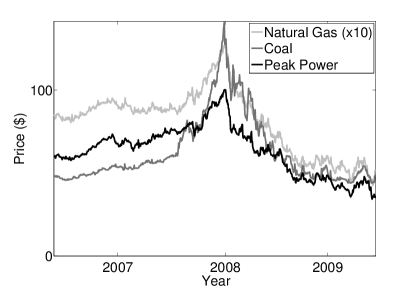
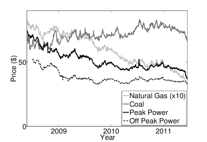
In the American PJM market, coal and gas are the fuel types most likely to be at the margin, with coal historically below gas in the merit order. Therefore PJM provides a suitable case study for analyzing the dependence structure suggested by our model. In Figure 5 we observe the historical co-movement of forward (futures) prices for PJM electricity (both peak and off-peak), Henry Hub natural gas (scaled up by a factor of ten) and Central Appalachian coal. We pick maturities December 2009 and 2011, and plot futures prices over the two years just prior to maturity. Figure 5a covers the period 2007-09, characterized by a peak during the summer of 2008, when most commodities set new record highs. Gas, coal and power all moved fairly similarly during this two-year period, although the correlation between power and gas forward prices is most striking.
Refer to caption
(a) Dec 2009 forward price dynamics.
Refer to caption
(b) Dec 2011 forward price dynamics.
Figure 5. Comparison of power, gas and coal futures prices for two delivery dates

Figure 5b depicts the period 2009-2011, during which, due primarily to shale gas discoveries, gas prices declined steadily through 2010 and 2011, while coal prices held steady and even increased a little. As a result, this period is more revealing, as it corresponds to a time of gradual change in the merit order. Our bid stack model implies that the level of power prices should have been impacted both by the strengthening coal price and the falling gas price, leading to a relatively flat power price trajectory. This is precisely what Figure 5b reveals, with very stable forward power prices during 2010-2011. The close correlation with gas is still visible, but power prices did not fall as much as gas, as they were supported by the price of coal. Finally, we can also see that the spread between peak and off-peak forwards for Dec 2011 delivery has narrowed significantly, as we would also expect when there is more overlap between coal and gas bids in the stack. This subtle change in price dynamics is crucial for many companies exposed to multi-commodity risk, and is one which is very difficult to capture in a typical reduced-form approach, or indeed in a stack model without a flexible merit order and overlapping fuel types.

5. Spread Options

This section deals with the pricing of spread options in the structural setting presented above. We are concerned with spread options whose payoff is defined to be the positive part of the difference between the market spot price of electricity and the cost of the amount of fuel needed by a particular power plant to generate one MWh. If coal (gas) is the fuel featured in the payoff then the option is known as a dark (spark) spread. Denoting by hc,hg>0subscript𝑐subscript𝑔0h_{c},h_{g}>0 the heat rate of coal or gas, dark and spark spread options with maturity T𝑇T have payoffs

(12) (PThcSTc)+and(PThgSTg)+,superscriptsubscript𝑃𝑇subscript𝑐subscriptsuperscript𝑆𝑐𝑇andsuperscriptsubscript𝑃𝑇subscript𝑔subscriptsuperscript𝑆𝑔𝑇\left(P_{T}-h_{c}S^{c}_{T}\right)^{+}\quad\text{and}\quad\left(P_{T}-h_{g}S^{g}_{T}\right)^{+},

respectively. We only consider the dark spread but point out that all results in this section apply to spark spreads if one interchanges c𝑐c and g𝑔g. Further, since spread options are typically traded to hedge physical assets (generating units) the heat rates that feature in the option payoff are usually in line with the efficiency of power plants in the market. Based on the range of market heat rates implied by our stack model, we require333Explicit formulae for cases of hcsubscript𝑐h_{c} outside of this range are also available, but not included here.

(13) exp(kc)hcexp(kc+mcξ¯c).subscript𝑘𝑐subscript𝑐subscript𝑘𝑐subscript𝑚𝑐superscript¯𝜉𝑐\exp\left(k_{c}\right)\leq h_{c}\leq\exp\left(k_{c}+m_{c}\bar{\xi}^{c}\right).

Then, as usually, the value (Vt)subscript𝑉𝑡(V_{t}) of a dark spread is given by the conditional expectation under the pricing measure of the discounted payoff; i.e.

Vt=exp(r(Tt))𝔼[(PThcSTc)+|t],subscript𝑉𝑡𝑟𝑇𝑡superscript𝔼delimited-[]conditionalsuperscriptsubscript𝑃𝑇subscript𝑐subscriptsuperscript𝑆𝑐𝑇subscript𝑡V_{t}=\exp\left(-r(T-t)\right)\mathbb{E}^{\mathbb{Q}}\left[\left.\left(P_{T}-h_{c}S^{c}_{T}\right)^{+}\right|\mathcal{F}_{t}\right],

which thanks to Corollary 2 is understood to be a derivative written on demand and fuels.

Remark 6.

While spread option contracts are often written on forwards, we consider spread options on spot prices, as required for our goal of power plant valuation. In addition, as we are interested in closed-form expressions, we limit our attention to the payoffs with strike zero, corresponding to a plant for which fixed operating costs are negligible or relatively small. Including a positive strike, one requires approximation techniques to price a spread option explicitly (such as perturbation of the strike zero case), analogously to approaches proposed for when both commodities are lognormal (cf. [9]).

5.1. Closed Form Spread Option Prices

The results derived in this section mirror those in §4.1 derived for the forward contract. Firstly, conditioning on demand, we obtain an explicit formula for the price of the spread. Secondly, we extend this result to give a closed form formula in the case of truncated Gaussian demand.

We keep our earlier notation for the dominant and subordinate technology i+subscript𝑖i_{+} and isubscript𝑖i_{-}, and define

ξh:=loghckcmc,assignsuperscript𝜉subscript𝑐subscript𝑘𝑐subscript𝑚𝑐\xi^{h}:=\frac{\log h_{c}-k_{c}}{m_{c}},

where 0ξhξ¯c0superscript𝜉superscript¯𝜉𝑐0\leq\xi^{h}\leq\bar{\xi}^{c}. By its definition, ξhsuperscript𝜉\xi^{h} represents the amount of electricity that can be supplied in the market from coal generators whose heat rate is smaller than or equal to hcsubscript𝑐h_{c}.

Proposition 3.

Given I={c,g}𝐼𝑐𝑔I=\{c,g\}, if, under \mathbb{Q}, the random variables log(STc)subscriptsuperscript𝑆𝑐𝑇\log(S^{c}_{T}) and log(STg)subscriptsuperscript𝑆𝑔𝑇\log(S^{g}_{T}) are jointly Gaussian distributed with means μcsubscript𝜇𝑐\mu_{c} and μgsubscript𝜇𝑔\mu_{g}, variances σc2superscriptsubscript𝜎𝑐2\sigma_{c}^{2} and σg2superscriptsubscript𝜎𝑔2\sigma_{g}^{2} and correlation ρ𝜌\rho, then, for t[0,T]𝑡0𝑇t\in[0,T], the price of a dark spread option with maturity T𝑇T is given by

(14) Vt=exp(r(Tt)){0min(ξ¯g,ξh)vlow,2(D,𝐅t)ϕd(D)dD+min(ξ¯g,ξh)ξ¯ivlow,1(D,𝐅t)ϕd(D)dD+ξ¯imax(ξ¯g,ξh)vmid,3(D,𝐅t)ϕd(D)dD+max(ξ¯g,ξh)min(ξ¯g+ξh,ξ¯c)vmid,2,i+(D,𝐅t)ϕd(D)dD+min(ξ¯g+ξh,ξ¯c)ξ¯i+vmid,1(D,𝐅t)ϕd(D)dD+ξ¯i+max(ξ¯c,ξ¯g+ξh)vhigh,2(D,𝐅t)ϕd(D)dD+max(ξ¯c,ξ¯g+ξh)ξ¯vhigh,1(D,𝐅t)ϕd(D)dD},subscript𝑉𝑡𝑟𝑇𝑡superscriptsubscript0superscript¯𝜉𝑔superscript𝜉subscript𝑣low2𝐷subscript𝐅𝑡subscriptitalic-ϕ𝑑𝐷d𝐷superscriptsubscriptsuperscript¯𝜉𝑔superscript𝜉superscript¯𝜉subscript𝑖subscript𝑣low1𝐷subscript𝐅𝑡subscriptitalic-ϕ𝑑𝐷differential-d𝐷superscriptsubscriptsuperscript¯𝜉subscript𝑖superscript¯𝜉𝑔superscript𝜉subscript𝑣mid3𝐷subscript𝐅𝑡subscriptitalic-ϕ𝑑𝐷differential-d𝐷superscriptsubscriptsuperscript¯𝜉𝑔superscript𝜉superscript¯𝜉𝑔superscript𝜉superscript¯𝜉𝑐subscript𝑣mid2subscript𝑖𝐷subscript𝐅𝑡subscriptitalic-ϕ𝑑𝐷differential-d𝐷superscriptsubscriptsuperscript¯𝜉𝑔superscript𝜉superscript¯𝜉𝑐superscript¯𝜉subscript𝑖subscript𝑣mid1𝐷subscript𝐅𝑡subscriptitalic-ϕ𝑑𝐷differential-d𝐷superscriptsubscriptsuperscript¯𝜉subscript𝑖superscript¯𝜉𝑐superscript¯𝜉𝑔superscript𝜉subscript𝑣high2𝐷subscript𝐅𝑡subscriptitalic-ϕ𝑑𝐷d𝐷superscriptsubscriptsuperscript¯𝜉𝑐superscript¯𝜉𝑔superscript𝜉¯𝜉subscript𝑣high1𝐷subscript𝐅𝑡subscriptitalic-ϕ𝑑𝐷d𝐷V_{t}=\exp\left(-r(T-t)\right)\left\{\int_{0}^{\min\left(\bar{\xi}^{g},\xi^{h}\right)}v_{\text{low},2}\left(D,\mathbf{F}_{t}\right)\phi_{d}(D)\ \mathrm{d}D\right.\\ +\int_{\min\left(\bar{\xi}^{g},\xi^{h}\right)}^{\bar{\xi}^{i_{-}}}v_{\text{low},1}\left(D,\mathbf{F}_{t}\right)\phi_{d}(D)\ \mathrm{d}D+\int_{\bar{\xi}^{i_{-}}}^{\max\left(\bar{\xi}^{g},\xi^{h}\right)}v_{\text{mid},3}\left(D,\mathbf{F}_{t}\right)\phi_{d}(D)\ \mathrm{d}D\\ +\int_{\max\left(\bar{\xi}^{g},\xi^{h}\right)}^{\min\left(\bar{\xi}^{g}+\xi^{h},\bar{\xi}^{c}\right)}v_{\text{mid},2,i_{+}}\left(D,\mathbf{F}_{t}\right)\phi_{d}(D)\ \mathrm{d}D+\int_{\min\left(\bar{\xi}^{g}+\xi^{h},\bar{\xi}^{c}\right)}^{\bar{\xi}^{i_{+}}}v_{\text{mid},1}\left(D,\mathbf{F}_{t}\right)\phi_{d}(D)\ \mathrm{d}D\\ +\int_{\bar{\xi}^{i_{+}}}^{\max\left(\bar{\xi}^{c},\bar{\xi}^{g}+\xi^{h}\right)}v_{\text{high},2}\left(D,\mathbf{F}_{t}\right)\phi_{d}(D)\ \mathrm{d}D+\left.\int_{\max\left(\bar{\xi}^{c},\bar{\xi}^{g}+\xi^{h}\right)}^{\bar{\xi}}v_{\text{high},1}\left(D,\mathbf{F}_{t}\right)\phi_{d}(D)\ \mathrm{d}D\right\},

where the integrands are given in Appendix B and discussed in some detail.

Proof.

As in the proof of Proposition 2, by iterated conditioning, for t[0,T]𝑡0𝑇t\in[0,T], the price of the dark spread Vtsubscript𝑉𝑡V_{t} is given by

Vt::subscript𝑉𝑡absent\displaystyle V_{t}: =exp(r(Tt))𝔼[(PThcSTc)+|t]absent𝑟𝑇𝑡superscript𝔼delimited-[]conditionalsuperscriptsubscript𝑃𝑇subscript𝑐subscriptsuperscript𝑆𝑐𝑇subscript𝑡\displaystyle=\exp\left(-r(T-t)\right)\mathbb{E}^{\mathbb{Q}}\left[\left.\left(P_{T}-h_{c}S^{c}_{T}\right)^{+}\right|\mathcal{F}_{t}\right]
=exp(r(Tt))𝔼[𝔼[(b(DT,𝐒T)hcSTc)+|T0tW]t].absent𝑟𝑇𝑡superscript𝔼delimited-[]superscript𝔼delimited-[]conditionalsuperscript𝑏subscript𝐷𝑇subscript𝐒𝑇subscript𝑐subscriptsuperscript𝑆𝑐𝑇subscriptsuperscript0𝑇subscriptsuperscript𝑊𝑡subscript𝑡\displaystyle=\exp\left(-r(T-t)\right)\mathbb{E}^{\mathbb{Q}}\left[\mathbb{E}^{\mathbb{Q}}\left[\left.\left(b(D_{T},\mathbf{S}_{T})-h_{c}S^{c}_{T}\right)^{+}\right|\mathcal{F}^{0}_{T}\vee\mathcal{F}^{W}_{t}\right]\mathcal{F}_{t}\right].

Again we write the outer expectation as the sum of integrals corresponding to the different forms the payoff can take, since the functional form of b𝑏b is different for DTsubscript𝐷𝑇D_{T} lying in the intervals [0,ξ¯i]0superscript¯𝜉subscript𝑖[0,\bar{\xi}^{i_{-}}], [ξ¯i,ξ¯i+]superscript¯𝜉subscript𝑖superscript¯𝜉subscript𝑖[\bar{\xi}^{i_{-}},\bar{\xi}^{i_{+}}], and [ξ¯i+,ξ¯]superscript¯𝜉subscript𝑖¯𝜉[\bar{\xi}^{i_{+}},\bar{\xi}]. In addition the functional form of the payoff now depends on whether DTξhsubscript𝐷𝑇superscript𝜉D_{T}\leq\xi^{h} or DTξhsubscript𝐷𝑇superscript𝜉D_{T}\geq\xi^{h} and on the magnitude of ξhsuperscript𝜉\xi^{h} relative to ξ¯csuperscript¯𝜉𝑐\bar{\xi}^{c} and ξ¯gsuperscript¯𝜉𝑔\bar{\xi}^{g}. Therefore, the first case is subdivided into the intervals [0,min(ξ¯g,ξh)]0superscript¯𝜉𝑔superscript𝜉[0,\min(\bar{\xi}^{g},\xi^{h})], and [min(ξ¯g,ξh),ξ¯i]superscript¯𝜉𝑔superscript𝜉superscript¯𝜉subscript𝑖[\min(\bar{\xi}^{g},\xi^{h}),\bar{\xi}^{i_{-}}]; the second case is subdivided into [ξ¯i,max(ξ¯g,ξh)]superscript¯𝜉subscript𝑖superscript¯𝜉𝑔superscript𝜉[\bar{\xi}^{i_{-}},\max(\bar{\xi}^{g},\xi^{h})], [max(ξ¯g,ξh),min(ξ¯g+ξh,ξ¯c)]superscript¯𝜉𝑔superscript𝜉superscript¯𝜉𝑔superscript𝜉superscript¯𝜉𝑐[\max(\bar{\xi}^{g},\xi^{h}),\min(\bar{\xi}^{g}+\xi^{h},\bar{\xi}^{c})], and [min(ξ¯g+ξh,ξ¯c),ξ¯i+]superscript¯𝜉𝑔superscript𝜉superscript¯𝜉𝑐superscript¯𝜉subscript𝑖[\min(\bar{\xi}^{g}+\xi^{h},\bar{\xi}^{c}),\bar{\xi}^{i_{+}}]; the third case is subdivided into [ξ¯i+,max(ξ¯c,ξ¯g+ξh)]superscript¯𝜉subscript𝑖superscript¯𝜉𝑐superscript¯𝜉𝑔superscript𝜉[\bar{\xi}^{i_{+}},\max(\bar{\xi}^{c},\bar{\xi}^{g}+\xi^{h})], and [max(ξ¯c,ξ¯g+ξh),ξ¯]superscript¯𝜉𝑐superscript¯𝜉𝑔superscript𝜉¯𝜉[\max(\bar{\xi}^{c},\bar{\xi}^{g}+\xi^{h}),\bar{\xi}].

The integrands v𝑣v in (14) are obtained by calculating the inner expectation for each demand interval listed above, in a similar fashion as in Proposition 2. ∎

Note that (14) requires seven terms in order to cover all possible values of hcsubscript𝑐h_{c} within the range given by (13), as well as the two cases c=i+𝑐subscript𝑖c=i_{+} and c=i𝑐subscript𝑖c=i_{-}. However, only five of the seven terms appear at once, with only the second or third appearing (depending on hcexp(kc+mcξ¯g)less-than-or-greater-thansubscript𝑐subscript𝑘𝑐subscript𝑚𝑐superscript¯𝜉𝑔h_{c}\lessgtr\exp(k_{c}+m_{c}\bar{\xi}^{g})) and only the fifth or sixth (depending on hcexp(kc+mc(ξ¯cξ¯g))less-than-or-greater-thansubscript𝑐subscript𝑘𝑐subscript𝑚𝑐superscript¯𝜉𝑐superscript¯𝜉𝑔h_{c}\lessgtr\exp(k_{c}+m_{c}(\bar{\xi}^{c}-\bar{\xi}^{g}))). These conditions can equivalently be written as ξhξ¯gless-than-or-greater-thansuperscript𝜉superscript¯𝜉𝑔\xi^{h}\lessgtr\bar{\xi}^{g} and ξhξ¯cξ¯gless-than-or-greater-thansuperscript𝜉superscript¯𝜉𝑐superscript¯𝜉𝑔\xi^{h}\lessgtr\bar{\xi}^{c}-\bar{\xi}^{g}. Notice that if c=i𝑐subscript𝑖c=i_{-}, we deduce that ξh<ξ¯gsuperscript𝜉superscript¯𝜉𝑔\xi^{h}<\bar{\xi}^{g} and ξh>ξ¯cξ¯gsuperscript𝜉superscript¯𝜉𝑐superscript¯𝜉𝑔\xi^{h}>\bar{\xi}^{c}-\bar{\xi}^{g} irrespective of hcsubscript𝑐h_{c}, while for c=i+𝑐subscript𝑖c=i_{+} several cases are possible.

Similar to the analysis of the forward contract earlier, if demand is assumed to be deterministic, then the spread option price is given explicitly by choosing the appropriate integrand from Proposition 2. To now obtain a convenient closed-form result for unknown demand, we extend our earlier notational tool for combining Gaussian distribution functions. For any integer n𝑛n, let

Φ22×n([x11x12x1nx21x22x2n],y;ρ)=i=1n[Φ2(x1i,y;ρ)Φ2(x2i,y;ρ)].superscriptsubscriptΦ22𝑛delimited-[]subscript𝑥11subscript𝑥12subscript𝑥1𝑛subscript𝑥21subscript𝑥22subscript𝑥2𝑛𝑦𝜌superscriptsubscript𝑖1𝑛delimited-[]subscriptΦ2subscript𝑥1𝑖𝑦𝜌subscriptΦ2subscript𝑥2𝑖𝑦𝜌\Phi_{2}^{2\times n}\left(\left[\begin{array}[]{cccc}x_{11}&x_{12}&\cdots&x_{1n}\\ x_{21}&x_{22}&\cdots&x_{2n}\end{array}\right],y;\rho\right)=\sum_{i=1}^{n}\left[\Phi_{2}(x_{1i},y;\rho)-\Phi_{2}(x_{2i},y;\rho)\right].

In addition, we introduce the following notation to capture all the relevant limits of integration. Define the vector 𝐚:=(a1,,a8)assign𝐚subscript𝑎1subscript𝑎8\mathbf{a}:=(a_{1},\ldots,a_{8}) by

𝐚:=1σd[(0,ξ¯gξh,ξ¯i,ξ¯gξh,ξ¯c(ξ¯g+ξh),ξ¯i+,ξ¯c(ξ¯g+ξh),ξ¯)μd].assign𝐚1subscript𝜎𝑑delimited-[]0superscript¯𝜉𝑔superscript𝜉superscript¯𝜉subscript𝑖superscript¯𝜉𝑔superscript𝜉superscript¯𝜉𝑐superscript¯𝜉𝑔superscript𝜉superscript¯𝜉subscript𝑖superscript¯𝜉𝑐superscript¯𝜉𝑔superscript𝜉¯𝜉subscript𝜇𝑑\mathbf{a}:=\frac{1}{\sigma_{d}}\left[\left(\begin{array}[]{cccccccc}0,&\bar{\xi}^{g}\wedge\xi^{h},&\bar{\xi}^{i_{-}},&\bar{\xi}^{g}\vee\xi^{h},&\bar{\xi}^{c}\wedge(\bar{\xi}^{g}+\xi^{h}),&\bar{\xi}^{i_{+}},&\bar{\xi}^{c}\vee(\bar{\xi}^{g}+\xi^{h}),&\bar{\xi}\end{array}\right)-\mu_{d}\right].

Notice that the components of 𝐚𝐚\mathbf{a} are in increasing order and correspond to the limits of integration in equation (14). In the case that c=i+𝑐subscript𝑖c=i_{+}, all of these values are needed, while the case c=i𝑐subscript𝑖c=i_{-} is somewhat simpler because a3=a4subscript𝑎3subscript𝑎4a_{3}=a_{4} and a5=a6subscript𝑎5subscript𝑎6a_{5}=a_{6} (since by (13), ξh<ξ¯csuperscript𝜉superscript¯𝜉𝑐\xi^{h}<\bar{\xi}^{c}). However, the result below is valid in both cases as various terms simply drop out in the latter case.

Corollary 4.

In addition to the assumptions in Proposition 3 let demand at maturity satisfy

DT=max(0,min(ξ¯,XT)),subscript𝐷𝑇0¯𝜉subscript𝑋𝑇D_{T}=\max\left(0,\min\left(\bar{\xi},X_{T}\right)\right),

where XTN(μd,σd2)similar-tosubscript𝑋𝑇𝑁subscript𝜇𝑑superscriptsubscript𝜎𝑑2X_{T}\sim N(\mu_{d},\sigma_{d}^{2}) is independent of 𝐒Tsubscript𝐒𝑇\mathbf{S}_{T}. Then for t[0,T]𝑡0𝑇t\in[0,T], the price of a dark spread is given explicitly by

Vt=exp(r(Tt)){bc(μd,Ftc)exp(mc2σd22)Φ22×2([ξ¯ca3a4a2],Rc(μd,0)mc2σd2σc,d;mcσdσc,d)+bc(μdξ¯g,Ftc)exp(mc2σd22)Φ22×2([a8a6a7a5],Rc(μdξ¯g,ξ¯g)+mc2σd2σc,d;mcσdσc,d)+bg(μdξ¯c,Ftg)exp(mg2σd22)Φ22×1([a8ξ¯c],Rg(μdξ¯c,ξ¯c)+mg2σd2σg,d;mgσdσg,d)hcFtcΦ22×3([a7a5a3a6a4a2],R~c((loghcβγμd)/αg)σg,γ;γσdαgσg,γ)+bcg(μd,𝐅t)exp(η){Φ22×2([ξ¯ca3a4a2],Rc(μd,0)αgσ2+γmcσd2σc,d;mcσdσc,d)Φ22×2([a8a6a7a5],Rc(μdξ¯g,ξ¯g)αgσ2+γmcσd2σc,d;mcσdσc,d)+Φ22×1([a8ξ¯c],Rg(μdξ¯c,ξ¯c)+αcσ2γmgσd2σg,d;mgσdσg,d)Φ22×3([a7a5a3a6a4a2],R~c((logHβγμd)/αg)αgσ2γ2σd2/αgσg,γ;γσdαgσg,γ)}+Φ1(a8)iIbi(ξ¯i,Fti)Φ1(Ri(ξ¯i,ξ¯j)σ)hcFtc(1Φ1(a7)+Φ1(a6)Φ1(a5))},subscript𝑉𝑡𝑟𝑇𝑡subscript𝑏𝑐subscript𝜇𝑑superscriptsubscript𝐹𝑡𝑐superscriptsubscript𝑚𝑐2superscriptsubscript𝜎𝑑22superscriptsubscriptΦ222delimited-[]superscript¯𝜉𝑐subscript𝑎3subscript𝑎4subscript𝑎2subscript𝑅𝑐subscript𝜇𝑑0superscriptsubscript𝑚𝑐2superscriptsubscript𝜎𝑑2subscript𝜎𝑐𝑑subscript𝑚𝑐subscript𝜎𝑑subscript𝜎𝑐𝑑subscript𝑏𝑐subscript𝜇𝑑superscript¯𝜉𝑔superscriptsubscript𝐹𝑡𝑐superscriptsubscript𝑚𝑐2superscriptsubscript𝜎𝑑22superscriptsubscriptΦ222delimited-[]subscript𝑎8subscript𝑎6subscript𝑎7subscript𝑎5subscript𝑅𝑐subscript𝜇𝑑superscript¯𝜉𝑔superscript¯𝜉𝑔superscriptsubscript𝑚𝑐2superscriptsubscript𝜎𝑑2subscript𝜎𝑐𝑑subscript𝑚𝑐subscript𝜎𝑑subscript𝜎𝑐𝑑subscript𝑏𝑔subscript𝜇𝑑superscript¯𝜉𝑐superscriptsubscript𝐹𝑡𝑔superscriptsubscript𝑚𝑔2superscriptsubscript𝜎𝑑22superscriptsubscriptΦ221delimited-[]subscript𝑎8superscript¯𝜉𝑐subscript𝑅𝑔subscript𝜇𝑑superscript¯𝜉𝑐superscript¯𝜉𝑐superscriptsubscript𝑚𝑔2superscriptsubscript𝜎𝑑2subscript𝜎𝑔𝑑subscript𝑚𝑔subscript𝜎𝑑subscript𝜎𝑔𝑑subscript𝑐superscriptsubscript𝐹𝑡𝑐superscriptsubscriptΦ223delimited-[]subscript𝑎7subscript𝑎5subscript𝑎3subscript𝑎6subscript𝑎4subscript𝑎2subscript~𝑅𝑐subscript𝑐𝛽𝛾subscript𝜇𝑑subscript𝛼𝑔subscript𝜎𝑔𝛾𝛾subscript𝜎𝑑subscript𝛼𝑔subscript𝜎𝑔𝛾subscript𝑏𝑐𝑔subscript𝜇𝑑subscript𝐅𝑡𝜂superscriptsubscriptΦ222delimited-[]superscript¯𝜉𝑐subscript𝑎3subscript𝑎4subscript𝑎2subscript𝑅𝑐subscript𝜇𝑑0subscript𝛼𝑔superscript𝜎2𝛾subscript𝑚𝑐superscriptsubscript𝜎𝑑2subscript𝜎𝑐𝑑subscript𝑚𝑐subscript𝜎𝑑subscript𝜎𝑐𝑑superscriptsubscriptΦ222delimited-[]subscript𝑎8subscript𝑎6subscript𝑎7subscript𝑎5subscript𝑅𝑐subscript𝜇𝑑superscript¯𝜉𝑔superscript¯𝜉𝑔subscript𝛼𝑔superscript𝜎2𝛾subscript𝑚𝑐superscriptsubscript𝜎𝑑2subscript𝜎𝑐𝑑subscript𝑚𝑐subscript𝜎𝑑subscript𝜎𝑐𝑑superscriptsubscriptΦ221delimited-[]subscript𝑎8superscript¯𝜉𝑐subscript𝑅𝑔subscript𝜇𝑑superscript¯𝜉𝑐superscript¯𝜉𝑐subscript𝛼𝑐superscript𝜎2𝛾subscript𝑚𝑔superscriptsubscript𝜎𝑑2subscript𝜎𝑔𝑑subscript𝑚𝑔subscript𝜎𝑑subscript𝜎𝑔𝑑superscriptsubscriptΦ223delimited-[]subscript𝑎7subscript𝑎5subscript𝑎3subscript𝑎6subscript𝑎4subscript𝑎2subscript~𝑅𝑐𝐻𝛽𝛾subscript𝜇𝑑subscript𝛼𝑔subscript𝛼𝑔superscript𝜎2superscript𝛾2superscriptsubscript𝜎𝑑2subscript𝛼𝑔subscript𝜎𝑔𝛾𝛾subscript𝜎𝑑subscript𝛼𝑔subscript𝜎𝑔𝛾subscriptΦ1subscript𝑎8subscript𝑖𝐼subscript𝑏𝑖superscript¯𝜉𝑖subscriptsuperscript𝐹𝑖𝑡subscriptΦ1subscript𝑅𝑖superscript¯𝜉𝑖superscript¯𝜉𝑗𝜎subscript𝑐superscriptsubscript𝐹𝑡𝑐1subscriptΦ1subscript𝑎7subscriptΦ1subscript𝑎6subscriptΦ1subscript𝑎5V_{t}=\exp\left(-r(T-t)\right)\left\{b_{c}\left(\mu_{d},F_{t}^{c}\right)\exp\left(\frac{m_{c}^{2}\sigma_{d}^{2}}{2}\right)\Phi_{2}^{2\times 2}\left(\left[\begin{array}[]{cc}\bar{\xi}^{c}&a_{3}\\ a_{4}&a_{2}\end{array}\right],\frac{R_{c}(\mu_{d},0)-m_{c}^{2}\sigma_{d}^{2}}{\sigma_{c,d}};\frac{m_{c}\sigma_{d}}{\sigma_{c,d}}\right)\right.\\ +b_{c}\left(\mu_{d}-\bar{\xi}^{g},F_{t}^{c}\right)\exp\left(\frac{m_{c}^{2}\sigma_{d}^{2}}{2}\right)\Phi_{2}^{2\times 2}\left(\left[\begin{array}[]{cc}a_{8}&a_{6}\\ a_{7}&a_{5}\end{array}\right],\frac{-R_{c}\left(\mu_{d}-\bar{\xi}^{g},\bar{\xi}^{g}\right)+m_{c}^{2}\sigma_{d}^{2}}{\sigma_{c,d}};\frac{-m_{c}\sigma_{d}}{\sigma_{c,d}}\right)\\ +b_{g}\left(\mu_{d}-\bar{\xi}^{c},F_{t}^{g}\right)\exp\left(\frac{m_{g}^{2}\sigma_{d}^{2}}{2}\right)\Phi_{2}^{2\times 1}\left(\left[\begin{array}[]{c}a_{8}\\ \bar{\xi}^{c}\end{array}\right],\frac{-R_{g}\left(\mu_{d}-\bar{\xi}^{c},\bar{\xi}^{c}\right)+m_{g}^{2}\sigma_{d}^{2}}{\sigma_{g,d}};\frac{-m_{g}\sigma_{d}}{\sigma_{g,d}}\right)\\ -h_{c}F_{t}^{c}\Phi_{2}^{2\times 3}\left(\left[\begin{array}[]{ccc}a_{7}&a_{5}&a_{3}\\ a_{6}&a_{4}&a_{2}\end{array}\right],\frac{\tilde{R}_{c}\left(\left(\log h_{c}-\beta-\gamma\mu_{d}\right)/\alpha_{g}\right)}{\sigma_{g,\gamma}};\frac{-\gamma\sigma_{d}}{\alpha_{g}\sigma_{g,\gamma}}\right)\\ +b_{cg}\left(\mu_{d},\mathbf{F}_{t}\right)\exp\left(\eta\right)\left\{\Phi_{2}^{2\times 2}\left(\left[\begin{array}[]{cc}\bar{\xi}^{c}&a_{3}\\ a_{4}&a_{2}\end{array}\right],\frac{-R_{c}(\mu_{d},0)-\alpha_{g}\sigma^{2}+\gamma m_{c}\sigma_{d}^{2}}{\sigma_{c,d}};\frac{-m_{c}\sigma_{d}}{\sigma_{c,d}}\right)\right.\\ -\Phi_{2}^{2\times 2}\left(\left[\begin{array}[]{cc}a_{8}&a_{6}\\ a_{7}&a_{5}\end{array}\right],\frac{-R_{c}\left(\mu_{d}-\bar{\xi}^{g},\bar{\xi}^{g}\right)-\alpha_{g}\sigma^{2}+\gamma m_{c}\sigma_{d}^{2}}{\sigma_{c,d}};\frac{-m_{c}\sigma_{d}}{\sigma_{c,d}}\right)\\ +\Phi_{2}^{2\times 1}\left(\left[\begin{array}[]{c}a_{8}\\ \bar{\xi}^{c}\end{array}\right],\frac{R_{g}\left(\mu_{d}-\bar{\xi}^{c},\bar{\xi}^{c}\right)+\alpha_{c}\sigma^{2}-\gamma m_{g}\sigma_{d}^{2}}{\sigma_{g,d}};\frac{m_{g}\sigma_{d}}{\sigma_{g,d}}\right)\\ -\left.\Phi_{2}^{2\times 3}\left(\left[\begin{array}[]{ccc}a_{7}&a_{5}&a_{3}\\ a_{6}&a_{4}&a_{2}\end{array}\right],\frac{-\tilde{R}_{c}\left((\log H-\beta-\gamma\ \mu_{d})/\alpha_{g}\right)-\alpha_{g}\sigma^{2}-\gamma^{2}\sigma_{d}^{2}/\alpha_{g}}{\sigma_{g,\gamma}};\frac{\gamma\sigma_{d}}{\alpha_{g}\sigma_{g,\gamma}}\right)\right\}\\ +\left.\Phi_{1}\left(-a_{8}\right)\sum_{i\in I}b_{i}\left(\bar{\xi}^{i},F^{i}_{t}\right)\Phi_{1}\left(\frac{-R_{i}\left(\bar{\xi}^{i},\bar{\xi}^{j}\right)}{\sigma}\right)-h_{c}F_{t}^{c}\left(1-\Phi_{1}\left(a_{7}\right)+\Phi_{1}(a_{6})-\Phi_{1}(a_{5})\right)\right\},

where

Ri~(z):=z+log(Ftj)log(Fti)12σ2andσi,γ2:=γ2σd2/αi2+σ2.formulae-sequenceassign~subscript𝑅𝑖𝑧𝑧subscriptsuperscript𝐹𝑗𝑡subscriptsuperscript𝐹𝑖𝑡12superscript𝜎2andassignsuperscriptsubscript𝜎𝑖𝛾2superscript𝛾2superscriptsubscript𝜎𝑑2superscriptsubscript𝛼𝑖2superscript𝜎2\tilde{R_{i}}(z):=z+\log\left(F^{j}_{t}\right)-\log\left(F^{i}_{t}\right)-\frac{1}{2}\sigma^{2}\quad\text{and}\quad\sigma_{i,\gamma}^{2}:=\gamma^{2}\sigma_{d}^{2}/\alpha_{i}^{2}+\sigma^{2}.
Proof.

All terms in (14) have the same form as those in Proposition 2 for forwards: demand appears linearly inside each Gaussian distribution function and in the exponential function multiplying it. Hence, applying Lemma 1 and simplifying lead to the result in the corollary. ∎

Remark 7.

Under the extended model introduced in §3.3 to capture spikes, spread prices are given by the same expression as in Proposition 4 plus the following simple terms444We require only two of the four extra terms in Remark 4 due to our assumption on hcsubscript𝑐h_{c} in (13), which guarantees that for the spike regime, the option is always in the money, while for the negative price regime, it never is. Hence, if we were to consider put spread options instead of calls, the other two terms would be needed instead.

exp(ms(μdξ¯)+12ms2σd2)Φ1(μdξ¯σd+msσd)Φ1(μdξ¯σd).subscript𝑚𝑠subscript𝜇𝑑¯𝜉12superscriptsubscript𝑚𝑠2superscriptsubscript𝜎𝑑2subscriptΦ1subscript𝜇𝑑¯𝜉subscript𝜎𝑑subscript𝑚𝑠subscript𝜎𝑑subscriptΦ1subscript𝜇𝑑¯𝜉subscript𝜎𝑑\exp\left(m_{s}(\mu_{d}-\bar{\xi})+\frac{1}{2}m_{s}^{2}\sigma_{d}^{2}\right)\Phi_{1}\left(\frac{\mu_{d}-\bar{\xi}}{\sigma_{d}}+m_{s}\sigma_{d}\right)-\Phi_{1}\left(\frac{\mu_{d}-\bar{\xi}}{\sigma_{d}}\right).

6. Numerical Analysis of Spread Option Prices

In this section, we investigate the implications of the two-fuel exponential stack model of §3.2 on spread option prices and power plant valuation, as compared to two common alternative approaches. We analyse prices for various parameter choices and option characteristics, as well as fuel forward curve scenarios.

Recall that the closed-form spread option prices given by Corollary 4 required no specification of a stochastic model for fuel prices, but instead imposed only a lognormality condition at maturity T𝑇T. However, for the purpose of comparing prices across maturities and across modeling approaches, we select a simple example of fuel price dynamics consistent with Corollary 4. We assume coal (Stc)subscriptsuperscript𝑆𝑐𝑡(S^{c}_{t}) and gas (Stg)subscriptsuperscript𝑆𝑔𝑡(S^{g}_{t}) follow correlated exponential OU processes under the measure \mathbb{Q}. i.e., for iI𝑖𝐼i\in I and t[0,T]𝑡0𝑇t\in[0,T],

(15) d(logSti)dsubscriptsuperscript𝑆𝑖𝑡\displaystyle\mathrm{d}(\log S^{i}_{t}) =\displaystyle= κi(λi(logSti))dt+νidWti,S0i=sisubscript𝜅𝑖subscript𝜆𝑖subscriptsuperscript𝑆𝑖𝑡d𝑡subscript𝜈𝑖dsubscriptsuperscript𝑊𝑖𝑡subscriptsuperscript𝑆𝑖0superscript𝑠𝑖\displaystyle\kappa_{i}\left(\lambda_{i}-(\log S^{i}_{t})\right)\mathrm{d}t+\nu_{i}\mathrm{d}W^{i}_{t},\quad S^{i}_{0}=s^{i}

where dWc,Wgt=ϱdtdsubscriptsuperscript𝑊𝑐superscript𝑊𝑔𝑡italic-ϱd𝑡\mathrm{d}\left<W^{c},W^{g}\right>_{t}=\varrho\mathrm{d}t. As gas and coal are treated identically in the bid stack model, we consider the symmetric case in which all coal and gas parameters are equal,555While it is of course not realistic for gas and coal to have identical prices (typically differ by a magnitude of about ten and trade in different units), it is plausible that after adjusting for different heat rates, the coal and gas bids could indeed coincide and have similar volatility, make our symmetric case less hypothetical. including both the parameters in (15) and in the exponential fuel bid curves, defined in (5). All are listed in Table 2, with the exception of ϱitalic-ϱ\varrho, which we vary throughout our analysis. All prices are calculated for time t=0𝑡0t=0. Note that for a given maturity T𝑇T, the parameters μcsubscript𝜇𝑐\mu_{c}, μgsubscript𝜇𝑔\mu_{g}, σcsubscript𝜎𝑐\sigma_{c}, σgsubscript𝜎𝑔\sigma_{g}, and ρ𝜌\rho appearing in §4 and §5 are related to those in (15) by the following standard results (for iI𝑖𝐼i\in I):

μisubscript𝜇𝑖\displaystyle\mu_{i} =\displaystyle= siexp(κiT)+λi(1exp(κiT)),superscript𝑠𝑖subscript𝜅𝑖𝑇subscript𝜆𝑖1subscript𝜅𝑖𝑇\displaystyle s^{i}\exp\left(-\kappa_{i}T\right)+\lambda_{i}\left(1-\exp\left(-\kappa_{i}T\right)\right),
σi2superscriptsubscript𝜎𝑖2\displaystyle\sigma_{i}^{2} =\displaystyle= νi22κi(1exp(2κiT)),superscriptsubscript𝜈𝑖22subscript𝜅𝑖12subscript𝜅𝑖𝑇\displaystyle\frac{\nu_{i}^{2}}{2\kappa_{i}}\left(1-\exp\left(-2\kappa_{i}T\right)\right),
ρσcσg𝜌subscript𝜎𝑐subscript𝜎𝑔\displaystyle\rho\sigma_{c}\sigma_{g} =\displaystyle= ϱνcνgκc+κg(1exp(κcTκgT)).italic-ϱsubscript𝜈𝑐subscript𝜈𝑔subscript𝜅𝑐subscript𝜅𝑔1subscript𝜅𝑐𝑇subscript𝜅𝑔𝑇\displaystyle\frac{\varrho\nu_{c}\nu_{g}}{\kappa_{c}+\kappa_{g}}\left(1-\exp\left(-\kappa_{c}T-\kappa_{g}T\right)\right).

As for fuel prices, recall that no particular process is required for electricity demand in our model. Typically driven by temperature, demand is often modelled as rapidly mean-reverting to a seasonal level. Hence, in our examples, we assume (Xt)subscript𝑋𝑡(X_{t}), as introduced in Corollary 4, to be an independent OU process, with a high value for mean-reversion speed (e.g. 100 or more). For our aim of pricing options with maturities of several months or even years, the values of these parameters are insignificant, as DTsubscript𝐷𝑇D_{T} is always well approximated by its stationary distribution. Hence, in Table 2 we list only the values μdsubscript𝜇𝑑\mu_{d} and σdsubscript𝜎𝑑\sigma_{d}. We also assume the interest rate r=0𝑟0r=0 throughout. This completes the base parameter set to be used throughout this section unless otherwise stated.

Bid curves Fuel price processes Demand Rate
kisubscript𝑘𝑖k_{i} misubscript𝑚𝑖m_{i} ξ¯isuperscript¯𝜉𝑖\bar{\xi}^{i} κisubscript𝜅𝑖\kappa_{i} νisubscript𝜈𝑖\nu_{i} λisubscript𝜆𝑖\lambda_{i} sisuperscript𝑠𝑖s^{i} μdsubscript𝜇𝑑\mu_{d} σdsubscript𝜎𝑑\sigma_{d} r
2 1 0.5 1 0.5 log(10)10\log(10) 101010 0.5 0.2 0
Table 2. Parameters used throughout §6 (for iI𝑖𝐼i\in I)

Next, we introduce three scenarios designed to assess the role of observed fuel forward curves and corresponding implications for bid stack structure. Fuel forward curves reveal crucial information about the probability of future merit order changes. For example, if bids from coal and gas are currently at similar levels (as in our parameter set) but one fuel is in backwardation (forwards decreasing in T𝑇T), while the other is in contango (increasing in T𝑇T), then the future dynamics of power prices (under \mathbb{Q}) should reflect the high chance of the coal and gas bids separating. We compare the following scenarios:

  1. (I)

    No fuel forward inputs (forward prices implied from (15))

  2. (II)

    Gas in contango; coal in backwardation (linear with stepsize of 0.2 per month)

  3. (III)

    No fuel forwards, but gas bids above coal (λc=log(sc)=log(7)subscript𝜆𝑐superscript𝑠𝑐7\lambda_{c}=\log(s^{c})=\log(7), λg=log(sg)=log(13)subscript𝜆𝑔superscript𝑠𝑔13\lambda_{g}=\log(s^{g})=\log(13))

Note that in Scenario II, fuel forward curves are inputs assumed to be observed from the market, instead of being generated by a model. The standard approach to resolving the inconsistency between the market and the model in (15) is to calibrate to fuel forwards for each T𝑇T via a shift in the mean level μisubscript𝜇𝑖\mu_{i} (or more formally via a time dependent long-term mean λisubscript𝜆𝑖\lambda_{i}).

6.1. Spread Option Price Comparison

To test our model’s prices for spark and dark spread options, we compare with two other typical approaches to spread option pricing: Margrabe’s formula (cf. [25]) and a simple cointegration model (cf. [17], [15] for discussions of cointegration between electricity and fuels).

6.1.1. Margrabe’s Formula

Assume that under the measure \mathbb{Q}, the electricity price PTsubscript𝑃𝑇P_{T} and fuel price STisubscriptsuperscript𝑆𝑖𝑇S^{i}_{T}, iI𝑖𝐼i\in I, are jointly lognormal, with correlation ρp,isubscript𝜌𝑝𝑖\rho_{p,i}. Writing μpsubscript𝜇𝑝\mu_{p} and σp2superscriptsubscript𝜎𝑝2\sigma_{p}^{2} for the mean and variance of log(PT)subscript𝑃𝑇\log(P_{T}), then for t[0,T]𝑡0𝑇t\in[0,T], the price of a spread option with payoff (12) is given by

Vtm=exp(r(Tt))[FtpΦ1(log(Ftp/hiFti)+σp,i2/2σp,i)hiFtiΦ1(log(Ftp/hiFti)σp,i2/2σp,i)],subscriptsuperscript𝑉𝑚𝑡𝑟𝑇𝑡delimited-[]subscriptsuperscript𝐹𝑝𝑡subscriptΦ1superscriptsubscript𝐹𝑡𝑝subscript𝑖superscriptsubscript𝐹𝑡𝑖superscriptsubscript𝜎𝑝𝑖22subscript𝜎𝑝𝑖subscript𝑖subscriptsuperscript𝐹𝑖𝑡subscriptΦ1superscriptsubscript𝐹𝑡𝑝subscript𝑖superscriptsubscript𝐹𝑡𝑖superscriptsubscript𝜎𝑝𝑖22subscript𝜎𝑝𝑖V^{m}_{t}=\exp\left(-r(T-t)\right)\left[F^{p}_{t}\Phi_{1}\left(\frac{\log\left(F_{t}^{p}/h_{i}F_{t}^{i}\right)+\sigma_{p,i}^{2}/2}{\sigma_{p,i}}\right)-h_{i}F^{i}_{t}\Phi_{1}\left(\frac{\log\left(F_{t}^{p}/h_{i}F_{t}^{i}\right)-\sigma_{p,i}^{2}/2}{\sigma_{p,i}}\right)\right],

where σp,i2=σp22ρp,iσpσi+σi2superscriptsubscript𝜎𝑝𝑖2superscriptsubscript𝜎𝑝22subscript𝜌𝑝𝑖subscript𝜎𝑝subscript𝜎𝑖superscriptsubscript𝜎𝑖2\sigma_{p,i}^{2}=\sigma_{p}^{2}-2\rho_{p,i}\sigma_{p}\sigma_{i}+\sigma_{i}^{2}, and all other notation is as before.

6.1.2. Cointegration Model

Let YTsubscript𝑌𝑇Y_{T} be an independent Gaussian random variable under \mathbb{Q}, with mean μysubscript𝜇𝑦\mu_{y} and variance σy2superscriptsubscript𝜎𝑦2\sigma_{y}^{2}. Then for constant weights wc,wg>0subscript𝑤𝑐subscript𝑤𝑔0w_{c},w_{g}>0 (the cointegrating vector), we define PTsubscript𝑃𝑇P_{T} by

PT:=wcSTc+wgSTg+YT.assignsubscript𝑃𝑇subscript𝑤𝑐subscriptsuperscript𝑆𝑐𝑇subscript𝑤𝑔subscriptsuperscript𝑆𝑔𝑇subscript𝑌𝑇P_{T}:=w_{c}S^{c}_{T}+w_{g}S^{g}_{T}+Y_{T}.

No closed form results are available for spread options, so prices are determined by simulation.

6.1.3. Comments on Comparison Methodology

In order to achieve a sensible comparison between the stack model and either Margrabe or the cointegration model, the mean and variance of PTsubscript𝑃𝑇P_{T} should be chosen appropriately, for each maturity. For a single fixed T𝑇T this simply requires choosing parameters μpsubscript𝜇𝑝\mu_{p} and σpsubscript𝜎𝑝\sigma_{p} (in the case of Margrabe) or μysubscript𝜇𝑦\mu_{y} and σysubscript𝜎𝑦\sigma_{y} (in the case of the cointegration model) to exactly match the mean and the variance of PTsubscript𝑃𝑇P_{T} produced by the stack model. As we shall often compare models simultaneously across many maturities, we use a variation of this idea, finding the best fit of an OU process for log(Pt)subscript𝑃𝑡\log(P_{t}) or (Yt)subscript𝑌𝑡(Y_{t}). For Margrabe,

d(logPt)=κp(λp(logPt))dt+νpdWtp,P0=p0,formulae-sequencedsubscript𝑃𝑡subscript𝜅𝑝subscript𝜆𝑝subscript𝑃𝑡d𝑡subscript𝜈𝑝dsubscriptsuperscript𝑊𝑝𝑡subscript𝑃0subscript𝑝0\mathrm{d}(\log P_{t})=\kappa_{p}\left(\lambda_{p}-(\log P_{t})\right)\mathrm{d}t+\nu_{p}\mathrm{d}W^{p}_{t},\qquad P_{0}=p_{0},

where dWp,Wit=ϱp,idtdsubscriptsuperscript𝑊𝑝superscript𝑊𝑖𝑡subscriptitalic-ϱ𝑝𝑖d𝑡\mathrm{d}\left<W^{p},W^{i}\right>_{t}=\varrho_{p,i}\mathrm{d}t for iI𝑖𝐼i\in I, while for the cointegration case (Yt)subscript𝑌𝑡(Y_{t}) is an independent OU process. In all cases we utilize the closed form expression for the variance of PTsubscript𝑃𝑇P_{T} in the stack model, given in Appendix A.

Finally, to reflect the symmetry between coal and gas in our parameter set, in the cointegration model we set wc=wg=1/2exp(kc+mc(μdξ¯c))subscript𝑤𝑐subscript𝑤𝑔12subscript𝑘𝑐subscript𝑚𝑐subscript𝜇𝑑superscript¯𝜉𝑐w_{c}=w_{g}=1/2\exp(k_{c}+m_{c}(\mu_{d}\bar{\xi}^{c})), such that the power price has equal dependence on each fuel, with a price level linked to the most likely marginal bid levels of coal and gas. Note that since both underlying fuels appear in the cointegration model like in the stack model, a comparison across values of fuel price correlation ϱitalic-ϱ\varrho is quite natural. On the other hand, the correlation parameter which we vary in the Margrabe approach is ϱp,isubscriptitalic-ϱ𝑝𝑖\varrho_{p,i}, which correlates electricity and fuel. Hence the choices of ϱitalic-ϱ\varrho or ϱp,isubscriptitalic-ϱ𝑝𝑖\varrho_{p,i} in the following plots are not perfect comparisons, but rather illustrate the role of correlation in generating a range of prices for each model. Due to variations across maturities, there is no direct link between a chosen value ϱitalic-ϱ\varrho and an appropriate ϱp,isubscriptitalic-ϱ𝑝𝑖\varrho_{p,i} short of estimating these from data.

Refer to caption
(a) All models (Scenario I)
Refer to caption
(b) Stack model (μd=0.3subscript𝜇𝑑0.3\mu_{d}=0.3,σd=0.12subscript𝜎𝑑0.12\sigma_{d}=0.12)
Figure 6. Spread option prices against hisubscript𝑖h_{i} for different correlations and demand levels

6.2. Spread Option Parameter Analysis

6.2.1. Spread prices versus heat rate hisubscript𝑖h_{i}

For a fixed maturity T=1𝑇1T=1, we plot dark spread option prices as a function of heat rate hcsubscript𝑐h_{c} (over a range corresponding to (13)). Figure 6a illustrates the Scenario I results for each of the three models considered, for two different correlation parameters, ϱ=±0.8italic-ϱplus-or-minus0.8\varrho=\pm 0.8. In all three models, negative correlation logically raises the option price, as it increases the volatility of the spread. The stack model generally predicts lower spread option prices than Margrabe, and a smaller gap between different correlation levels. This is because the strong structural link keeps long-term levels of power and gas close together, thus narrowing the spread distribution relative to the weaker case of correlated Brownian Motions. The gap between Margrabe and the stack model widens with negative correlation, while for extreme positive correlation (not plotted), Margrabe can underprice the stack model. Another way of understanding this phenomenon is to notice that the bid stack automatically imposes a positive dependence structure between electricity and its underlying fuels, which can only be somewhat weakened or strengthened by varying fuel price correlation through ϱitalic-ϱ\varrho. The cointegration approach shares this characteristic, and therefore prices much closer to the stack model than Margrabe, but still somewhat higher for ϱ=0.8italic-ϱ0.8\varrho=0.8.

Unlike for Margrabe, Figure 6b reveals interestingly that the dependence on correlation ϱitalic-ϱ\varrho does not hold strictly for the stack model, as exceptions can be found. Considering a market with very low demand (μd=0.3,σd=0.12)\mu_{d}=0.3,\sigma_{d}=0.12), we observe that the relationship with ϱitalic-ϱ\varrho is reversed for low values of hcsubscript𝑐h_{c}. Since demand is so low, the price is typically set by the cheaper fuel and hence only in the money for coal bids generally below gas. Hence for negative ϱitalic-ϱ\varrho, we do not receive the typical high payoffs from high gas and low coal states, and get zero payoff when coal moves above gas in the stack. Figure 6b also confirms that this reversal is most pronounced if coal bids are shifted to be below gas bids, as described by Scenario III.
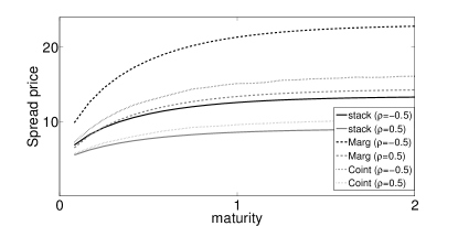
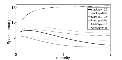
Refer to caption
(a) Scenario I: Spark or dark spread
Refer to caption
(b) Scenario II: Spark spread
Figure 7. Option prices against T𝑇T for different correlations and fuel forward scenarios

6.2.2. Spread prices versus maturity T𝑇T

We next investigate spread option prices against maturity T𝑇T, and for this purpose fix hi=exp(ki+miξ¯i/2)subscript𝑖subscript𝑘𝑖subscript𝑚𝑖superscript¯𝜉𝑖2h_{i}=\exp(k_{i}+m_{i}\bar{\xi}^{i}/2) in option payoffs, matching the median heat rate in the market. We again compare several correlation levels for all three models, and now include Scenario II to test the impact of fuel forward curves. In Figure 7a (Scenario I), spread options are typically increasing in maturity as expected, and flatten out as the price processes approach their stationary distributions, with an ordering of the three models resembling Figure 6a. More interestingly, in Scenario II (Figure 7b), longer term spark spread options drop significantly in value in stack model, are thus greatly overpriced by Margrabe, and significantly overpriced by the cointegration model as well. As the gas forward curve is now in contango, while coal is in backwardation, coal will almost always be below gas in the future bid stack, especially for very long maturities. Hence, a spark spread option has relatively little chance of being in the money, as this would require unusually high demand. This is a good example of a dependency which cannot be captured by Margrabe or other reduced-form models, but is automatically captured by the merit order built into the stack model. Moreover, fuel forward prices are direct inputs into our expressions for spread options, avoiding the need for an additional calibration step to first match observed fuel forwards, as is the case for the other approaches.
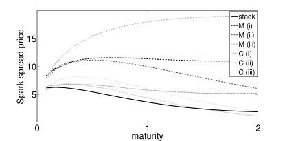
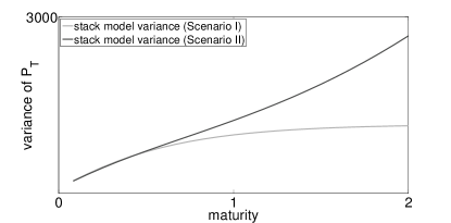
Refer to caption
(a) Scenario II: Spark Spread Comparison
Refer to caption
(b) Comparison of variances
Figure 8. Analysis of impact of matching mean and variance of PTsubscript𝑃𝑇P_{T} for Scenario II

So far all plots have assumed that both the mean and variance of the power price distributions are matched in all three models, via the procedure described in Section 6.1.3. One might question whether this is realistic. In practice, we only have history (and possibly observed forward curves) to calibrate each model, and thus should not be borrowing extra information about the future from the stack model’s structure when calibrating the other approaches. While matching the mean is reasonable as it is analogous to matching observed power forwards, matching the variance is less justifiable. In Figure 8a, we compare spark spread option prices for Margrabe and the cointegration model in Scenario II (as in Figure 7b but now ρ=0𝜌0\rho=0) for three different calibration assumptions: full matching as earlier; matching means but not variances; matching neither means nor variances. Here ‘not matched’ implies that means and/or variances are instead fitted to Scenario I levels (a proxy for history). We note significant differences between all cases. Failing to match the mean implies a greater overpricing of spark spreads in this case, while failing to match the variances acts in the opposite direction here, lowering the price since the forward looking variance (implied by the stack in Scenario II) is higher than the variance in Scenario I (see Figure 8b). While other scenarios could lead to different patterns, it is clear that significant price differences can occur due to the likely changes in the merit order. In Margrabe, no information is transmitted from fuel forward prices to the distribution of PTsubscript𝑃𝑇P_{T}, while in the cointegration model limited information is transmitted, since the relative dependence on coal and gas is fixed initially by wc,wgsubscript𝑤𝑐subscript𝑤𝑔w_{c},w_{g}, instead of dynamically adapting to fuel price movements (and demand). In contrast, the stack model produces highly state-dependent power price volatility and correlations reflecting known information about the future market structure.
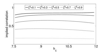
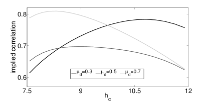
Refer to caption
(a) Implied correlation varying ξ¯gsuperscript¯𝜉𝑔\bar{\xi}^{g}
Refer to caption
(b) Implied correlation varying μdsubscript𝜇𝑑\mu_{d}
Refer to caption
(c) ϱimpsuperscriptitalic-ϱ𝑖𝑚𝑝\varrho^{imp} surface (Scenario I)
Refer to caption
(d) ϱimpsuperscriptitalic-ϱ𝑖𝑚𝑝\varrho^{imp} surface (Scenario II)
Figure 9. Implied correlation analysis for various parameters and scenarios

6.3. Implied Correlation Analysis

We next analyse ‘implied correlation’ ϱp,iimpsubscriptsuperscriptitalic-ϱ𝑖𝑚𝑝𝑝𝑖\varrho^{imp}_{p,i}, meaning the value of ϱp,isubscriptitalic-ϱ𝑝𝑖\varrho_{p,i} for which Margrabe’s formula reproduces the stack model price. As Figures 6 and 7 suggest, for high (positive) values of ϱitalic-ϱ\varrho in the stack, it may be impossible for Margrabe to reproduce the price, for any ϱp,i[1,1]subscriptitalic-ϱ𝑝𝑖11\varrho_{p,i}\in[-1,1]. In such cases, implied correlation does not exist. However, ϱp,iimpsubscriptsuperscriptitalic-ϱ𝑖𝑚𝑝𝑝𝑖\varrho^{imp}_{p,i} typically exists for most values of ϱitalic-ϱ\varrho, and can be understood as a convenient way of measuring (or quoting) the gap between Margrabe and the stack model price.

In Figures 9a-9b, we investigate implied correlation ‘smiles’ (against hcsubscript𝑐h_{c}) for a dark spread option in Scenario I and with ϱ=0italic-ϱ0\varrho=0. In Figure 9a we first vary the relative capacities of coal and gas (with ξ¯=1¯𝜉1\bar{\xi}=1 throughout). In all cases Margrabe overprices the spread since ϱp,cimp>0subscriptsuperscriptitalic-ϱ𝑖𝑚𝑝𝑝𝑐0\varrho^{imp}_{p,c}>0, but the difference is much larger when coal is the dominant technology. As we approach the case of a dark spread in a fully gas driven market (ξ¯gsuperscript¯𝜉𝑔\bar{\xi}^{g} near 1), Margrabe approaches the stack price (ρimpsuperscript𝜌𝑖𝑚𝑝\rho^{imp} near 0). In Figure 9b we assume ξ¯c=ξ¯g=0.5superscript¯𝜉𝑐superscript¯𝜉𝑔0.5\bar{\xi}^{c}=\bar{\xi}^{g}=0.5, but instead vary μdsubscript𝜇𝑑\mu_{d} (with σdsubscript𝜎𝑑\sigma_{d} now 0.12). We see that the implied correlation has a slight downward (upward) skew if demand is high (low), and a fairly symmetric ‘frown’ for μd=0.5subscript𝜇𝑑0.5\mu_{d}=0.5. Figures 9c-9d plot implied correlation as a function of both hh and T𝑇T for Scenarios I and II. When given fuel forward curves as inputs (Scenario II), we can observe a distinctive tilt in the implied correlation surface for long maturities.

6.4. Power Plant Valuation

We conclude this analysis with an investigation into the bid stack model’s predictions for power plant valuation under our chosen scenarios. A generating unit of fuel type iI𝑖𝐼i\in I, with heat rate hisubscript𝑖h_{i}, can be approximated as a sum of spread options on spot power (cf. [19])). Letting {Tj:jJ}conditional-setsubscript𝑇𝑗𝑗𝐽\{T_{j}:j\in J\} represent all future hours of production over the plant’s life, the plant value (VPt)𝑉subscript𝑃𝑡(VP_{t}) for t[0,T]𝑡0𝑇t\in[0,T] is then

VPt=jJexp(r(Tjt))𝔼[(PTjhiSTji)+|t]𝑉subscript𝑃𝑡subscript𝑗𝐽𝑟subscript𝑇𝑗𝑡superscript𝔼delimited-[]conditionalsuperscriptsubscript𝑃subscript𝑇𝑗subscript𝑖subscriptsuperscript𝑆𝑖subscript𝑇𝑗subscript𝑡VP_{t}=\sum_{j\in J}\exp\left(-r(T_{j}-t)\right)\mathbb{E}^{\mathbb{Q}}\left[\left.\left(P_{T_{j}}-h_{i}S^{i}_{T_{j}}\right)^{+}\right|\mathcal{F}_{t}\right]

While this approximation technique ignores complicated operational constraints, it is consistent with our approximation of the electricity price setting mechanism itself, since a plant bidding at cost every day receives exactly this string of payoffs in our model.
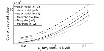
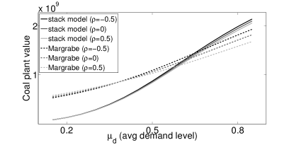
Refer to caption
(a) Scenario I
Refer to caption
(b) Scenario II (Coal Plant)
Refer to caption
(c) Scenario III (Coal Plant)
Refer to caption
(d) Scenario III (Gas Plant)
Figure 10. Power Plant Value (3yrs, 1000MW) as a function of μdsubscript𝜇𝑑\mu_{d} for various scenarios

In Figure 10 we value a 1000 MW power plant with a life of three years in the Margrabe case and stack model, exploiting our closed-form formulas for reasonable computation time. Instead of making an arbitrary assumption about the important periodicities of power demand (which vary from market to market) we use a fixed mean μdsubscript𝜇𝑑\mu_{d} for all hours in each calculation, but investigate the resulting plant value as a function of μdsubscript𝜇𝑑\mu_{d}. We also fix hi=exp(ki+miξ¯i/2)subscript𝑖subscript𝑘𝑖subscript𝑚𝑖superscript¯𝜉𝑖2h_{i}=\exp(k_{i}+m_{i}\bar{\xi}^{i}/2) throughout. In Scenario I (Figure 10a), Margrabe prices consistently higher than the stack model as expected. Figure 10b considers Scenario II where fuel forward prices pull future gas and coal bids in opposite directions, and Margrabe matches the distribution of PTsubscript𝑃𝑇P_{T} only from history. Remarkably, for long enough maturities and high enough μdsubscript𝜇𝑑\mu_{d}, Margrabe sometimes underprices a coal power plant relative to the stack model. Here the stack captures that gas is likely to be the marginal fuel in the future, with coal plants operating near full capacity.

Another interesting case to consider is Scenario III, in which there is very little overlap between coal and gas bids to begin with, and coal is likely to remain below gas in the merit order. Figures 10c-10d reveal the result of this change. Unsurprisingly, for a gas power plant (Figure 10d) the deviation between the stack model and Margrabe is large, since the gas plant has little chance of being called upon to produce power. On the other hand, the difference between Margrabe and the stack model is much less for the coal plant, and the stack model price appears to converge to Margrabe for high demand (similarly to Figure 9a for high ξ¯gsuperscript¯𝜉𝑔\bar{\xi}^{g}). The reason for this is that when coal is always below gas in the stack and demand always high, then the power price can be approximated by the gas stack alone. Hence, power price should be close to lognormal and the correlation between power and coal close to that of gas and coal. Furthermore, as there is no mismatch of mean or variance (as there was in 10b), under such a scenario, Margrabe’s formula should give a very similar price to the stack model.

Finally, it is important to remember the heavy-tailed nature of most electricity spot prices, which makes a lognormal distribution for PTsubscript𝑃𝑇P_{T} highly questionable. As discussed in Section 3.3, the bid stack model allows for a straightforward extension to capture spikes (or negative prices) consistently without limiting the availability of derivative pricing formulae. To illustrate the impact of spikes, Figure 11 plots the same scenarios as in Figures 10a and 10d, except using our extended stack model666This implies a spike of about $150 in the event Xt=1.1ξ¯subscript𝑋𝑡1.1¯𝜉X_{t}=1.1\,\bar{\xi}, and so is a fairly conservative choice. Note also that we still match the mean of the Margrabe formula (i.e., calibrate to the stack model’s electricity forward curve), but only match the variance to the case of no spikes, since otherwise the fit to the new variance (with spikes) becomes infeasible for large μdsubscript𝜇𝑑\mu_{d}. with parameter ms=50subscript𝑚𝑠50m_{s}=50 (and σdsubscript𝜎𝑑\sigma_{d} reduced from 0.2 to 0.1). The impact of spikes is to shift the stack model valuation closer to Margrabe, but only in the case of high μdsubscript𝜇𝑑\mu_{d}. This is intuitive of course because spikes are only present for high enough demand. Since the stack model produces a heavier-tailed distribution for PTsubscript𝑃𝑇P_{T} than the lognormal, very high μdsubscript𝜇𝑑\mu_{d} can lead to stack model valuation even above Margrabe.
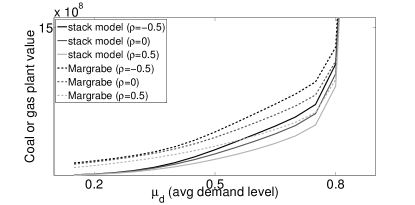
Refer to caption
(a) Scenario I
Refer to caption
(b) Scenario III (Gas Plant)
Figure 11. Power plant value with stack model extended to include spike regime

7. Conclusion

The valuation and hedging of both physical and financial assets in electricity markets is a complex and highly state-dependent challenge, particularly for medium to long term problems in markets driven by multiple underlying fuels. As we have seen in the examples of §6, it is important to be aware of the current merit order and resulting bid stack shape, as well as likely or possible changes to this order in the future. Observed fuel forward curves can provide valuable information for this purpose, but cannot be incorporated easily into traditional reduced-form models for power prices. On the other hand, a structural approach maintains a close link with the physical characteristics of the electricity market, allowing for the inclusion of a variety of forward looking information, such as demand forecasts, or changes in the generation mix of the market, a pertinent issue in many countries nowadays. The piecewise exponential bid stack model proposed here achieves this link, while crucially retaining closed-form expressions for forwards and spread options, as presented in Sections 4 and 5. In this way, it enjoys the benefits of a simple reduced-form model, while mimicking the complex dependence structure produced by a full production cost optimization model, for which derivative pricing is typically a computationally infeasible task. Furthermore, the availability of explicit expressions for forwards and options is highly beneficial for many other practical purposes, such as calibration to observed market quotes, the calculation of Greeks and for risk management applications (e.g. simulating price changes for a portfolio of physical assets). Although we focused primarily here on a simple coal and gas based market, we believe that our general framework has the flexibility to be adapted to various market conditions, as illustrated for example by our simple extension to capture extreme spikes at times of high demand, an important feature of most power markets. As we have shown through many examples, the delicate interplay between demand, capacity, and multiple fuel prices is embedded into our approach, thus providing an intuitive framework for understanding complicated interdependencies, while also helping to bridge the prevalent gap between mathematical tractability and the economics of supply and demand.

Appendix A Moments and Covariances

If demand at maturity satisfies

DT=max(0,min(ξ¯,XT)),subscript𝐷𝑇0¯𝜉subscript𝑋𝑇D_{T}=\max\left(0,\min\left(\bar{\xi},X_{T}\right)\right),

with XTN(μd,σd2)similar-tosubscript𝑋𝑇𝑁subscript𝜇𝑑superscriptsubscript𝜎𝑑2X_{T}\sim N(\mu_{d},\sigma_{d}^{2}) independent of 𝐒Tsubscript𝐒𝑇\mathbf{S}_{T}, then for t[0,T]𝑡0𝑇t\in[0,T], the n𝑛n-th moment of PTsubscript𝑃𝑇P_{T} is given by

𝔼[PTn|t]=Φ1(μdσd)iIbin(0,Fti)exp(12(n2n)σi2)Φ1(Ri(n)(0,0)σ)+Φ1(μdξ¯σd)iIbin(ξ¯i,Fti)exp(12(n2n)σi2)Φ1(Ri(n)(ξ¯i,ξ¯i)σ)+iIbin(μd,Fti)exp(ζi(n))Φ22×1([ξ¯iμdσdnmiσdμdσdnmiσd],Ri(n)(μd,0)nmi2σd2σi,d;miσdσi,d)+iIbin(μdξ¯j,Fti)exp(ζi(n))Φ22×1([ξ¯μdσdnmiσdξ¯jμdσdnmiσd],Ri(n)(μdξ¯j,ξ¯j)+nmi2σd2σi,d;miσdσi,d)+iIδibcgn(μd,𝐅t)exp(η(n)){Φ22×1([ξ¯iμdσdnγσdμdσdnγσd],Ri(μd,0)+nαjσ2nγmiσd2δiσi,d;miσdδiσi,d)+Φ22×1([ξ¯μdσdnγσdξ¯jμdσdnγσd],Ri(μdξ¯j,ξ¯j)+nαjσ2nγmiσd2δiσi,d;miσdδiσi,d)},𝔼delimited-[]conditionalsuperscriptsubscript𝑃𝑇𝑛subscript𝑡subscriptΦ1subscript𝜇𝑑subscript𝜎𝑑subscript𝑖𝐼subscriptsuperscript𝑏𝑛𝑖0subscriptsuperscript𝐹𝑖𝑡12superscript𝑛2𝑛superscriptsubscript𝜎𝑖2subscriptΦ1subscriptsuperscript𝑅𝑛𝑖00𝜎subscriptΦ1subscript𝜇𝑑¯𝜉subscript𝜎𝑑subscript𝑖𝐼subscriptsuperscript𝑏𝑛𝑖superscript¯𝜉𝑖subscriptsuperscript𝐹𝑖𝑡12superscript𝑛2𝑛superscriptsubscript𝜎𝑖2subscriptΦ1subscriptsuperscript𝑅𝑛𝑖superscript¯𝜉𝑖superscript¯𝜉𝑖𝜎subscript𝑖𝐼subscriptsuperscript𝑏𝑛𝑖subscript𝜇𝑑superscriptsubscript𝐹𝑡𝑖superscriptsubscript𝜁𝑖𝑛superscriptsubscriptΦ221delimited-[]superscript¯𝜉𝑖subscript𝜇𝑑subscript𝜎𝑑𝑛subscript𝑚𝑖subscript𝜎𝑑subscript𝜇𝑑subscript𝜎𝑑𝑛subscript𝑚𝑖subscript𝜎𝑑subscriptsuperscript𝑅𝑛𝑖subscript𝜇𝑑0𝑛superscriptsubscript𝑚𝑖2superscriptsubscript𝜎𝑑2subscript𝜎𝑖𝑑subscript𝑚𝑖subscript𝜎𝑑subscript𝜎𝑖𝑑subscript𝑖𝐼subscriptsuperscript𝑏𝑛𝑖subscript𝜇𝑑superscript¯𝜉𝑗subscriptsuperscript𝐹𝑖𝑡superscriptsubscript𝜁𝑖𝑛superscriptsubscriptΦ221delimited-[]¯𝜉subscript𝜇𝑑subscript𝜎𝑑𝑛subscript𝑚𝑖subscript𝜎𝑑superscript¯𝜉𝑗subscript𝜇𝑑subscript𝜎𝑑𝑛subscript𝑚𝑖subscript𝜎𝑑subscriptsuperscript𝑅𝑛𝑖subscript𝜇𝑑superscript¯𝜉𝑗superscript¯𝜉𝑗𝑛superscriptsubscript𝑚𝑖2superscriptsubscript𝜎𝑑2subscript𝜎𝑖𝑑subscript𝑚𝑖subscript𝜎𝑑subscript𝜎𝑖𝑑subscript𝑖𝐼subscript𝛿𝑖subscriptsuperscript𝑏𝑛𝑐𝑔subscript𝜇𝑑subscript𝐅𝑡superscript𝜂𝑛superscriptsubscriptΦ221delimited-[]superscript¯𝜉𝑖subscript𝜇𝑑subscript𝜎𝑑𝑛𝛾subscript𝜎𝑑subscript𝜇𝑑subscript𝜎𝑑𝑛𝛾subscript𝜎𝑑subscript𝑅𝑖subscript𝜇𝑑0𝑛subscript𝛼𝑗superscript𝜎2𝑛𝛾subscript𝑚𝑖superscriptsubscript𝜎𝑑2subscript𝛿𝑖subscript𝜎𝑖𝑑subscript𝑚𝑖subscript𝜎𝑑subscript𝛿𝑖subscript𝜎𝑖𝑑superscriptsubscriptΦ221delimited-[]¯𝜉subscript𝜇𝑑subscript𝜎𝑑𝑛𝛾subscript𝜎𝑑superscript¯𝜉𝑗subscript𝜇𝑑subscript𝜎𝑑𝑛𝛾subscript𝜎𝑑subscript𝑅𝑖subscript𝜇𝑑superscript¯𝜉𝑗superscript¯𝜉𝑗𝑛subscript𝛼𝑗superscript𝜎2𝑛𝛾subscript𝑚𝑖superscriptsubscript𝜎𝑑2subscript𝛿𝑖subscript𝜎𝑖𝑑subscript𝑚𝑖subscript𝜎𝑑subscript𝛿𝑖subscript𝜎𝑖𝑑\mathbb{E}[P_{T}^{n}|\mathcal{F}_{t}]=\Phi_{1}\left(\frac{-\mu_{d}}{\sigma_{d}}\right)\sum_{i\in I}b^{n}_{i}\left(0,F^{i}_{t}\right)\exp\left(\frac{1}{2}(n^{2}-n)\sigma_{i}^{2}\right)\Phi_{1}\left(\frac{R^{(n)}_{i}(0,0)}{\sigma}\right)\\ +\Phi_{1}\left(\frac{\mu_{d}-\bar{\xi}}{\sigma_{d}}\right)\sum_{i\in I}b^{n}_{i}\left(\bar{\xi}^{i},F^{i}_{t}\right)\exp\left(\frac{1}{2}(n^{2}-n)\sigma_{i}^{2}\right)\Phi_{1}\left(\frac{-R^{(n)}_{i}\left(\bar{\xi}^{i},\bar{\xi}^{i}\right)}{\sigma}\right)\\ +\sum_{i\in I}b^{n}_{i}\left(\mu_{d},F_{t}^{i}\right)\exp\left(\zeta_{i}^{(n)}\right)\Phi_{2}^{2\times 1}\left(\left[\begin{array}[]{c}\frac{\bar{\xi}^{i}-\mu_{d}}{\sigma_{d}}-nm_{i}\sigma_{d}\\ \frac{-\mu_{d}}{\sigma_{d}}-nm_{i}\sigma_{d}\end{array}\right],\frac{R^{(n)}_{i}(\mu_{d},0)-nm_{i}^{2}\sigma_{d}^{2}}{\sigma_{i,d}};\frac{m_{i}\sigma_{d}}{\sigma_{i,d}}\right)\\ +\sum_{i\in I}b^{n}_{i}\left(\mu_{d}-\bar{\xi}^{j},F^{i}_{t}\right)\exp\left(\zeta_{i}^{(n)}\right)\Phi_{2}^{2\times 1}\left(\left[\begin{array}[]{c}\frac{\bar{\xi}-\mu_{d}}{\sigma_{d}}-nm_{i}\sigma_{d}\\ \frac{\bar{\xi}^{j}-\mu_{d}}{\sigma_{d}}-nm_{i}\sigma_{d}\end{array}\right],\frac{-R^{(n)}_{i}(\mu_{d}-\bar{\xi}^{j},\bar{\xi}^{j})+nm_{i}^{2}\sigma_{d}^{2}}{\sigma_{i,d}};\frac{-m_{i}\sigma_{d}}{\sigma_{i,d}}\right)\\ +\sum_{i\in I}\delta_{i}b^{n}_{cg}\left(\mu_{d},\mathbf{F}_{t}\right)\exp\left(\eta^{(n)}\right)\left\{-\Phi_{2}^{2\times 1}\left(\left[\begin{array}[]{c}\frac{\bar{\xi}^{i}-\mu_{d}}{\sigma_{d}}-n\gamma\sigma_{d}\\ \frac{-\mu_{d}}{\sigma_{d}}-n\gamma\sigma_{d}\end{array}\right],\frac{R_{i}(\mu_{d},0)+n\alpha_{j}\sigma^{2}-n\gamma m_{i}\sigma_{d}^{2}}{\delta_{i}\sigma_{i,d}};\frac{m_{i}\sigma_{d}}{\delta_{i}\sigma_{i,d}}\right)\right.\\ +\left.\Phi_{2}^{2\times 1}\left(\left[\begin{array}[]{c}\frac{\bar{\xi}-\mu_{d}}{\sigma_{d}}-n\gamma\sigma_{d}\\ \frac{\bar{\xi}^{j}-\mu_{d}}{\sigma_{d}}-n\gamma\sigma_{d}\end{array}\right],\frac{R_{i}(\mu_{d}-\bar{\xi}^{j},\bar{\xi}^{j})+n\alpha_{j}\sigma^{2}-n\gamma m_{i}\sigma_{d}^{2}}{\delta_{i}\sigma_{i,d}};\frac{m_{i}\sigma_{d}}{\delta_{i}\sigma_{i,d}}\right)\right\},

where j=I{i}𝑗𝐼𝑖j=I\setminus\{i\}, δi=(1)𝕀{i=i+}subscript𝛿𝑖superscript1subscript𝕀𝑖subscript𝑖\delta_{i}=(-1)^{\mathbb{I}_{\{i=i_{+}\}}} as before and

Ri(n)(ξi,ξj)superscriptsubscript𝑅𝑖𝑛subscript𝜉𝑖subscript𝜉𝑗\displaystyle R_{i}^{(n)}(\xi_{i},\xi_{j}) :=kj+mjξjkimiξi+log(Ftj)log(Fti)(n12)σi212σj2+nρσiσj,assignabsentsubscript𝑘𝑗subscript𝑚𝑗subscript𝜉𝑗subscript𝑘𝑖subscript𝑚𝑖subscript𝜉𝑖subscriptsuperscript𝐹𝑗𝑡subscriptsuperscript𝐹𝑖𝑡𝑛12superscriptsubscript𝜎𝑖212superscriptsubscript𝜎𝑗2𝑛𝜌subscript𝜎𝑖subscript𝜎𝑗\displaystyle:=k_{j}+m_{j}\xi_{j}-k_{i}-m_{i}\xi_{i}+\log(F^{j}_{t})-\log(F^{i}_{t})-(n-\frac{1}{2})\sigma_{i}^{2}-\frac{1}{2}\sigma_{j}^{2}+n\rho\sigma_{i}\sigma_{j},
η(n)superscript𝜂𝑛\displaystyle\eta^{(n)} :=n22(γ2σd2αcαgσ2),andζi(n):=12(n2n)σi2+12n2mi2σd2.formulae-sequenceassignabsentsuperscript𝑛22superscript𝛾2superscriptsubscript𝜎𝑑2subscript𝛼𝑐subscript𝛼𝑔superscript𝜎2andassignsuperscriptsubscript𝜁𝑖𝑛12superscript𝑛2𝑛superscriptsubscript𝜎𝑖212superscript𝑛2superscriptsubscript𝑚𝑖2superscriptsubscript𝜎𝑑2\displaystyle:=\frac{n^{2}}{2}\left(\gamma^{2}\sigma_{d}^{2}-\alpha_{c}\alpha_{g}\sigma^{2}\right),\qquad\text{and}\qquad\zeta_{i}^{(n)}:=\frac{1}{2}(n^{2}-n)\sigma_{i}^{2}+\frac{1}{2}n^{2}m_{i}^{2}\sigma_{d}^{2}.

A more general formula for 𝔼[PTn(STc)nc(STg)ng|t]𝔼delimited-[]conditionalsuperscriptsubscript𝑃𝑇𝑛superscriptsuperscriptsubscript𝑆𝑇𝑐subscript𝑛𝑐superscriptsuperscriptsubscript𝑆𝑇𝑔subscript𝑛𝑔subscript𝑡\mathbb{E}[P_{T}^{n}(S_{T}^{c})^{n_{c}}(S_{T}^{g})^{n_{g}}|\mathcal{F}_{t}] can be obtained similarly, allowing us to calculate for example covariances between electricity and fuels.

Appendix B Terms in Spread Formula

The integrands in Proposition 4 correspond to the dark spread price in various demand intervals, in the case of a given or known demand value. These terms resemble those for forwards in Proposition 2, but can be categorized by whether the option is always, never or sometimes in the money for each case. For the last of these three cases, we have

vlow,1(ξ,𝐱)=bc(ξ,xc)Φ1(Rc(ξ,0)/σ)hcxcΦ1(R~c(h(ξ))/σ)subscript𝑣low1𝜉𝐱subscript𝑏𝑐𝜉superscript𝑥𝑐subscriptΦ1subscript𝑅𝑐𝜉0𝜎subscript𝑐superscript𝑥𝑐subscriptΦ1subscript~𝑅𝑐𝜉𝜎\displaystyle v_{\text{low},1}\left(\xi,\mathbf{x}\right)=b_{c}\left(\xi,x^{c}\right)\Phi_{1}\left(R_{c}(\xi,0)/\sigma\right)-h_{c}x^{c}\Phi_{1}\left(\tilde{R}_{c}\left(h(\xi)\right)/\sigma\right)
+bcg(ξ,𝐱)exp(σαcαg2)[1Φ1(Rc(ξ,0)/σαgσ)Φ1(R~g(h(ξ))/σαcσ)],subscript𝑏𝑐𝑔𝜉𝐱subscriptsuperscript𝜎2subscript𝛼𝑐subscript𝛼𝑔delimited-[]1subscriptΦ1subscript𝑅𝑐𝜉0𝜎subscript𝛼𝑔𝜎subscriptΦ1subscript~𝑅𝑔𝜉𝜎subscript𝛼𝑐𝜎\displaystyle\qquad+b_{cg}\left(\xi,\mathbf{x}\right)\exp\left(\sigma^{2}_{\alpha_{c}\alpha_{g}}\right)\left[1-\Phi_{1}\left(R_{c}(\xi,0)/\sigma-\alpha_{g}\sigma\right)-\Phi_{1}\left(\tilde{R}_{g}\left(h(\xi)\right)/\sigma-\alpha_{c}\sigma\right)\right],
vhigh,2(ξ,𝐱)=bg(ξξ¯c,xg)Φ1(Rg(ξξ¯c,ξ¯c)/σ)hcxcΦ1(R~c(h(ξ))/σ)subscript𝑣high2𝜉𝐱subscript𝑏𝑔𝜉superscript¯𝜉𝑐superscript𝑥𝑔subscriptΦ1subscript𝑅𝑔𝜉superscript¯𝜉𝑐superscript¯𝜉𝑐𝜎subscript𝑐superscript𝑥𝑐subscriptΦ1subscript~𝑅𝑐𝜉𝜎\displaystyle v_{\text{high},2}\left(\xi,\mathbf{x}\right)=b_{g}(\xi-\bar{\xi}^{c},x^{g})\Phi_{1}\left(-R_{g}\left(\xi-\bar{\xi}^{c},\bar{\xi}^{c}\right)/\sigma\right)-h_{c}x^{c}\Phi_{1}\left(\tilde{R}_{c}\left(h(\xi)\right)/\sigma\right)
+bcg(ξ,𝐱)exp(αcαgσ22)[Φ1(Rg(ξξ¯c,ξ¯c)/σαcσ)Φ1(R~g(h(ξ))/σαcσ)],subscript𝑏𝑐𝑔𝜉𝐱subscript𝛼𝑐subscript𝛼𝑔superscript𝜎22delimited-[]subscriptΦ1subscript𝑅𝑔𝜉superscript¯𝜉𝑐superscript¯𝜉𝑐𝜎subscript𝛼𝑐𝜎subscriptΦ1subscript~𝑅𝑔𝜉𝜎subscript𝛼𝑐𝜎\displaystyle\quad+b_{cg}\left(\xi,\mathbf{x}\right)\exp\left(-\frac{\alpha_{c}\alpha_{g}\sigma^{2}}{2}\right)\left[\Phi_{1}\left(R_{g}\left(\xi-\bar{\xi}^{c},\bar{\xi}^{c}\right)/\sigma-\alpha_{c}\sigma\right)-\Phi_{1}\left(\tilde{R}_{g}\left(h(\xi)\right)/\sigma-\alpha_{c}\sigma\right)\right],

and vmid,2,c=vlow,1subscript𝑣mid2𝑐subscript𝑣low1v_{\text{mid},2,c}=v_{\text{low},1}, vmid,2,g=vhigh,2subscript𝑣mid2𝑔subscript𝑣high2v_{\text{mid},2,g}=v_{\text{high},2}, where h(ξ)=(loghcβγξ)/αg𝜉subscript𝑐𝛽𝛾𝜉subscript𝛼𝑔h(\xi)=\left(\log h_{c}-\beta-\gamma\xi\right)/\alpha_{g}. Then

vmid,1(ξ,𝐱)=fmid(ξ,𝐱)hcxc,vhigh,1(ξ,𝐱)=fhigh(ξ,𝐱)hcxcformulae-sequencesubscript𝑣mid1𝜉𝐱subscript𝑓mid𝜉𝐱subscript𝑐superscript𝑥𝑐subscript𝑣high1𝜉𝐱subscript𝑓high𝜉𝐱subscript𝑐superscript𝑥𝑐v_{\text{mid},1}\left(\xi,\mathbf{x}\right)=f_{\text{mid}}\left(\xi,\mathbf{x}\right)-h_{c}x^{c},\qquad v_{\text{high},1}\left(\xi,\mathbf{x}\right)=f_{\text{high}}\left(\xi,\mathbf{x}\right)-h_{c}x^{c}

correspond to cases that are always in the money, while the following are never in the money:

vlow,2(ξ,𝐱)=vmid,3(ξ,𝐱)=0subscript𝑣low2𝜉𝐱subscript𝑣mid3𝜉𝐱0v_{\text{low},2}\left(\xi,\mathbf{x}\right)=v_{\text{mid},3}\left(\xi,\mathbf{x}\right)=0

Acknowledgements

This work was partially supported by the National Science Foundation grant DMS-0739195.

References

  • [1] Aïd, R., Campi, L., Huu, A.N., Touzi, N.: A structural risk-neutral model of electricity prices. International Journal of Theoretical and Applied Finance 12, 925–947 (2009)
  • [2] Aïd, R., Campi, L., Langrené, N.: A structural risk-neutral model for pricing and hedging power derivatives. Mathematical Finance (2012). To appear
  • [3] Barlow, M.: A diffusion model for electricity prices. Mathematical Finance 12, 287–298 (2002)
  • [4] Benth, F.E., Benth, J.S., Koekebakker, S.: Stochastic Modeling of Electricity and Related Markets. World Scientific Publishing Company (2008)
  • [5] Benth, F.E., Koekebakker, S.: Stochastic modeling of financial electricity contracts. Journal of Energy Economics 30, 1116–1157 (2007)
  • [6] Bessembinder, H., Lemmon, M.: Equilibrium pricing and optimal hedging in electricity forward markets. Journal of Finance 57(3), 1347–1382 (2002)
  • [7] Boogert, A., Dupont, D.: When supply meets demand: the case of hourly spot electricity prices. IEEE Transactions on Power Systems 23(2), 389–398 (2008)
  • [8] Burger, M., Klar, B., Müller, A., Schindlmayr, G.: A spot market model for pricing derivatives in electricity markets. Quantitative Finance 4, 109–122 (2004)
  • [9] Carmona, R., Durrleman, V.: Pricing and hedging spread options. SIAM Review 45, 627–685 (2003)
  • [10] Cartea, A., Figueroa, M.G., Geman, H.: Modelling electricity prices with forward looking capacity constraints. Applied Mathematical Finance 32, 2501–2519 (2008)
  • [11] Cartea, A., Villaplana, P.: Spot price modeling and the valuation of electricity forward contracts: the role of demand and capacity. Journal of Banking and Finance 32, 2501–2519 (2008)
  • [12] Clewlow, L., Strickland, C.: Energy derivatives. Tech. rep., Lacima Group (2000)
  • [13] Coulon, M.: Modelling price dynamics through fundamental relationships in electricity and other energy markets. Ph.D. thesis, University of Oxford (2009)
  • [14] Coulon, M., Howison, S.: Stochastic behaviour of the electricity bid stack: from fundamental drivers to power prices. Journal of Energy Markets 2, 29–69 (2009)
  • [15] De Jong, C., Schneider, S.: Cointegration between gas and power spot prices. Journal of Energy Markets 2(3), 27–46 (2009)
  • [16] Deng, S.: Stochastic models of energy commodity prices and their applications: Mean-reversion with jumps and spikes. Technical report, University of California Energy Institute (2003)
  • [17] Emery, G.W., Liu, Q.W.: An analysis of the relationship between electricity and natural-gas futures prices. The Journal of Futures Markets 22(2), 95–122 (2002)
  • [18] Eydeland, A., Geman, H.: Energy Modelling and the Management of Uncertainty, chap. Fundamentals of Electricity Derivatives, pp. 35–43. Risk Books (1999)
  • [19] Eydeland, A., Wolyniec, K.: Energy and Power Risk Management: New Developments in Modeling, Pricing and Hedging. John Wiley & Sons (2003)
  • [20] Frikha, N., Lemaire, V.: Joint modelling of gas and electricity spot prices. Applied Mathematical Finance
  • [21] Geske, R.: The valuation of compound options. Journal of Financial Economics 7, 63–81 (1979)
  • [22] Hortacsu, A., Puller, S.: Understanding strategic bidding in multi-unit auctions: A case study of the texas electricity market. The RAND Journal of Economics 39(1), 86–114 (2007)
  • [23] Howison, S., Schwarz, D.: Structural modelling of carbon emission markets. Working paper (2011)
  • [24] Lyle, M.R., Elliott, R.J.: A ”simple” hybrid model for power derivatives. Energy Economics 31, 757–767 (2009)
  • [25] Margrabe, W.: The value of an option to exchange one asset for another. The Journal of Finance 33, 177–186 (1978)
  • [26] Musiela, M., Rutkowski, M.: Martingale Methods in Financial Modelling. Springer (2009)
  • [27] Pirrong, C., Jermakyan, M.: The price of power: The valuation of power and weather derivatives. Journal of Banking and Finance 32, 2520–2529 (2008)
  • [28] Schwartz, E.: The stochastic behavior of commodity prices: Implications for valuation and hedging. The Journal of Finance 52, 923–973 (1997)
  • [29] Schwartz, E., Smith, J.E.: Short-term variations and long-term dynamics in commodity prices. Management Science 46, 893–911 (2000)
  • [30] Skantze, P., Gubina, A., Ilic, M.: Bid-based stochastic model for electricity prices: the impact of fundamental drivers on market dynamics. Mit e-lab report (2000)