Beyond-mean-field study of the possible “bubble” structure of ³⁴Si

Abstract

Recent self-consistent mean-field calculations predict a substantial depletion of the proton density in the interior of ${}^{34}\textrm{Si}$. In the present study, we investigate how correlations beyond the mean field modify this finding. The framework of the calculation is a particle-number and angular-momentum projected Generator Coordinate Method based on Hartree-Fock-Bogoliubov+Lipkin-Nogami states with axial quadrupole deformation. The parametrization SLy4 of the Skyrme energy density functional is used together with a density-dependent pairing energy functional. For the first time, the generator coordinate method is applied to the calculation of charge and transition densities. The impact of pairing correlations, symmetry restorations and shape mixing on the density profile is analyzed step by step. All these effects significantly alter the radial density profile, and tend to bring it closer to a Fermi-type density distribution.

I Introduction

Charge distributions in atomic nuclei Uberall71 ; Barrett74 ; Friar75 ; Sick85 ; Friedrich86 ; Frois87 ; Hodgson92 provide very detailed information about nuclear structure. They are obtained through the analysis of elastic electron-nucleus scattering data. Because of the absence of suitable targets, data on unstable nuclei are available, to the best of our knowledge, only for ${}^{14}\textrm{C}$ Kline73 and ${}^{3}\textrm{H}$ Beck87 ; Amrouna94 . The SCRIT project Wakasugi04 ; Suda05 ; Suda09 of constructing a high-resolution electron spectrometer that is underway in Japan and ELISe Antonov11 , planned to be constructed at FAIR, are expected to provide data about the charge distributions and transition form factors for many exotic nuclei in the future.

Because of the saturation properties of the nuclear medium, the radial dependence of the nuclear density takes, at the lowest order, the form of a Fermi distribution. However, the density often deviates from this simple behavior because of quantal effects related to the filling of single-particle states with wave functions that have specific spatial behavior. In this context, $s_{1/2}$ orbits in spherical nuclei have a very peculiar signature, as they are the only ones that contribute to the density at the nuclear center. Depending on whether they are filled or empty, $s_{1/2}$ orbits can generate a central bump in the density as it has been observed for ${}^{40}\textrm{Ca}$ Sick79 , or a central depression.

Mean-field-based methods Bender03 are the tools of choice when modeling the nuclear density distribution. Indeed, they include the ingredients required for this task: the full model space of occupied single-particle states as degrees of freedom together with an effective interaction that reproduces the empirical saturation properties of nuclear matter.

The density profile and the spatial dependence of the single-particle potentials are closely related and self-consistently linked to each other. A central depression in the density might be accompanied by two very specific properties of the mean-field potential, one related to its central part and a second one related to the spin-orbit potential.

A central depression of the density is reflected in the central potential by a maximum at the origin and a minimum for some finite distance $r$. This is often called a “wine-bottle” shaped central potential, referring to the shape of the bottom of a bottle of wine. Levels with low orbital angular momentum $\ell$ are then pushed up relatively to those with large $\ell$ that are pulled down. For sufficiently large rearrangement, the order of single-particle levels can even change, lowering the central density even more and leading to the so-called “bubble nuclei”. For specific “bubble magic numbers” 18, 34, 50, 58, 80, 120, …Wong72 ; Wong73 large shell effects might compensate for the loss in binding energy due to the reduced central density well below the nuclear matter saturation value. There was some speculation in the 1970s whether such structure could exist in nuclei that were about to become accessible for detailed studies, in particular ${}^{36}\textrm{Ar}$ and some Hg isotopes Wong72 ; Wong73 ; Davies72 ; Davies73 ; Campi73 ; Beiner73 ; Nilsson74 ; Saunier74 . However, the possibility of a bubble structure in these nuclei has been ruled out by experiment. By contrast, predictions that superheavy and hyperheavy nuclei beyond the currently known region of the mass table might take the form of bubbles Dietrich97 ; Decharge97 ; Bender99 ; Decharge03 ; Nazarewicz00 are still standing. In fact, for a large charge number $Z$, a hollow density distribution is energetically favored over a regular one as it lowers the Coulomb repulsion. In this context, one often distinguishes between “true bubbles”, which have vanishing density in their center, and “semi-bubbles”, which have a central density significantly lower than saturation density, but with a non-zero value.

The second effect of a central depression concerns the spin-orbit potential. In self-consistent mean-field models, this potential is proportional to the gradient of a combination of proton and neutron densities, whose relative weights depend on the model and parametrization Bender03 ; Bender99 . For nuclei with a regular density profile, it is peaked at the nuclear surface. For nuclei with a central depletion of the density, the spin-orbit potential has a second peak of opposite sign in the nuclear interior. This usually reduces the spin-orbit splitting of orbits located mainly at the nucleus center, whereas that of orbits situated at the nuclear surface is not affected.

Recently, there has been a renewal of interest in nuclei presenting a hollow in their density distributions. Some modern parametrizations of the relativistic mean field Todd-Rutel2004 ; Chu2010 and of the Skyrme energy density functional (EDF) Khan2008 ; Grasso2009 predict a hollow proton density for ${}^{34}\textrm{Si}$ and some neutron-rich Ar isotopes. At the time being, ${}^{34}\textrm{Si}$ stands out as the only candidate on which many different effective interactions agree. The possible proton bubble structure of this nucleus has also been suggested as an explanation of the results on the transfer reactions ${}^{36}\textrm{S}(d,p){}^{37}\textrm{S}$ and ${}^{34}\textrm{Si}(d,p){}^{35}\textrm{Si}$. Indeed, the splitting between the observed neutron $3/2^{-}$ and $1/2^{-}$ levels that have the largest spectroscopic factors in the $2p$ shell is decreased from ${}^{37}\textrm{S}$ ($\approx 1.7$ MeV) to ${}^{35}\textrm{Si}$ ($\approx 1.1$ MeV) Burgunder2011 ; Sorlin2011 .

Besides the debatable interaction dependence of the density distributions, one may wonder whether bubble-type structures are stable against correlation effects. Indeed, any correlation will inevitably populate empty levels and in particular the $2s_{1/2}$, even in models like the one that we use here, where its population cannot be easily singled out. In fact, it is known for a long time that, already for nuclei with a more regular density distribution, mean-field calculations tend to overestimate the spatial fluctuations of the density when compared to data. Correlations usually tend to flatten out the density distribution, and often bring it closer to data. The effect of pairing has been studied in Ref. Bennour89 , and the impact of fluctuations in shape degrees of freedom has been studied within the random phase approximation (RPA) for many spherical nuclei Faessler76 ; Reinhard79 ; Gogny79 ; Decharge83 ; Esbensen83 ; Johnson88 ; Barranco87 ; Sil08 and using a one-dimensional Girod76 or five-dimensional Gogny79 ; Decharge83 ; Girod82 microscopic collective Hamiltonian for some transitional ones.

The most obvious correlations that could reduce the central depression of the density are due to pairing Beiner73 . However, many calculations made for bubble nuclei do not include them Davies72 ; Davies73 ; Campi73 ; Saunier74 . This can be justified for ${}^{34}\textrm{Si}$, where the large gap between the proton $1d_{5/2}$ and $2s_{1/2}$ levels suppresses pairing, resulting in its unphysical collapse when treated with the Hartree-Fock-Bogoliubov (HFB) method. Pairing correlations have then to be treated beyond the mean field approximation. Another kind of correlations that might affect the density profile is related to the spreading of the ground-state wave function around the mean-field configuration. It has been pointed out in Ref. Bender06a that the ground states of most light nuclei may show strong shape fluctuations that in general lead to a substantial increase of their charge radii when treated in a beyond-mean-field framework. The same effect may also strongly influence the density profile.

In the following, we will compare results obtained from calculations that successively add correlations to the ground-state wave function:

1. spherical mean-field calculations without taking pairing correlations into account (HF)

2. spherical mean-field calculations including pairing correlations within the HFB+Lipkin-Nogami (HFB+LN) scheme, which constitutes an approximate variation after projection on particle number

3. particle-number projection after variation of the spherical mean-field state obtained in HFB+LN

4. configuration mixing of angular-momentum $J=0$ and particle-number projected mean-field states with different intrinsic axial quadrupole moment. We will refer to these wave functions in the following as symmetry-restored generator coordinate method (GCM).

In addition, we will study how much the observable charge density, obtained through convolution of the proton density with the proton’s internal charge distribution, differs from the point proton density used to calculate the energy.

Symmetry-restored GCM has been used to describe ground-state correlations and collective excitation spectra of a large range of nuclei with reasonable success Egido04 ; Bender08LH ; Niksic06 ; Bender2008 ; Rodriguez10 ; Yao10 . Its actual implementations are not yet flexible enough to reproduce correctly all details of excitation spectra, mainly because of the usually too low moment of inertia. However, this method describes rather well properties related to the nuclear shape, such as transition probabilities. It is therefore important to enlarge its range of applications by the calculation of charge and transition densities in the laboratory frame. In this paper, we report on a first application that enables us to illustrate the effect of various kinds of correlations on the density distribution of ${}^{34}\textrm{Si}$.

We will first give a brief outline of the model. Results for low-lying collective states in ${}^{34}\textrm{Si}$ are presented in Sect. III, whereas the modification of the ground state density distribution brought by correlations is discussed in Sect. IV. Section V will summarize our findings.

II Calculational details

The self-consistent HFB equations are solved on a cubic three-dimensional coordinate-space mesh extending from $-11.2$ fm to 11.2 fm in each direction with a step size of 0.8 fm. Thanks to the reflection symmetry with respect to the $x=0$, $y=0$ and $z=0$ planes imposed on the single-particle wave functions in our code Bonche05 , it is sufficient to solve the HFB equations in 1/8 of the box. The HFB equations are complemented by the Lipkin-Nogami prescription to avoid the unphysical breakdown of pairing correlations at low level density. A constraint on the axial mass quadrupole moment $q\equiv\langle Q_{2}\rangle=\langle 2z^{2}-x^{2}-y^{2}\rangle$ is used to construct mean-field states $|q\rangle$ with different intrinsic deformation.

Eigenstates of the particle-number operators $\hat{N}$ and $\hat{Z}$ are obtained by applying the projection operator

$$\hat{P}_{N_{0}}=\frac{1}{2\pi}\int_{0}^{2\pi}\!\!d\varphi\;e^{i\varphi(\hat{N}-N_{0})}$$ (1)

for neutrons and protons. Eigenstates of the total angular momentum in the laboratory frame $\hat{J}^{2}$ and its $z$ component $\hat{J}_{z}$ with eigenvalues $\hbar^{2}J(J+1)$ and $\hbar M$, respectively, are obtained by applying the operator

$$\hat{P}^{J}_{MK}=\frac{2J+1}{8\pi^{2}}\!\int_{0}^{2\pi}\!\!d\alpha\int_{0}^{\pi}\!\!d\beta\,\sin(\beta)\int_{0}^{2\pi}\!\!d\gamma\,\mathcal{D}^{J*}_{MK}\,\hat{R}$$ (2)

that contains the rotation operator $\hat{R}=e^{-i\alpha\hat{J}_{x}}\,e^{-i\beta\hat{J}_{y}}\,e^{-i\gamma\hat{J}_{z}}$ and the Wigner rotation matrix $\mathcal{D}^{J}_{MK}(\alpha,\beta,\gamma)$ on the nucleus’ wave function. Both depend on the Euler angles $\alpha$, $\beta$ and $\gamma$. The operator $\hat{P}^{J}_{MK}$ picks the component with projection $K$ along the intrinsic $z$ axis from the mean-field state. Throughout this study, we will restrict ourselves to axial states with $K=0$. As angular-momentum projected states will be always projected also on particle-number, we drop the indices $N_{0}$ and $Z_{0}$for the sake of notation:

$$|JMq\rangle=\frac{\hat{P}^{J}_{M0}\hat{P}_{N_{0}}\hat{P}_{Z_{0}}|q\rangle}{\sqrt{\langle q|\hat{P}^{J}_{00}\hat{P}_{N_{0}}\hat{P}_{Z_{0}}|q\rangle}}\,.$$ (3)

GCM Ring80 is a very flexible tool that in particular allows us to study the spreading of the mean-field ground-state wave function in collective degrees of freedom. It will be used here to study the fluctuations of the spherical ground state of ${}^{34}\textrm{Si}$ with respect to the axial quadrupole moment assuming a superposition of projected HFB+LN states of different deformation $|q\rangle$:

$$|JM\mu\rangle=\sum_{q}f_{\mu}^{J}(q)\,|JMq\rangle\,.$$ (4)

The weight factors $f_{\mu}^{J}(q)$ and the energies $E_{\mu}^{J}$ of the states $|JM\mu\rangle$ are the solutions of the Hill-Wheeler-Griffin equations Ring80

$$\sum_{q^{\prime}}\left[\mathcal{H}^{J}(q,q^{\prime})-E_{\mu}^{J}\mathcal{N}^{J}(q,q^{\prime})\right]\,f_{\mu}^{J}(q^{\prime})=0\,,$$ (5)

where the norm kernel reads $\mathcal{N}^{J}(q,q^{\prime})=\langle JMq|JMq^{\prime}\rangle$ and where the energy kernel is given by a multi-reference energy density functional that depends on the mixed density matrix between the two projected states $|JMq\rangle$ and $|JMq^{\prime}\rangle$ Lacroix09 .

Throughout this article, we will use the parametrization SLy4 Chabanat98 of the Skyrme energy density functional together with a local pairing energy functional of surface type Rigollet99 with parameters $\rho_{0}=0.16$ fm^-3 for the switching density and $V_{0}=-1000.0$ MeV fm³ for the pairing strength unless noted otherwise. A soft cutoff at $\pm 5$ MeV around the Fermi energy is used when solving the HFB equations as described in Ref. Rigollet99 . More details about the calculations of the GCM kernels can be found in Ref. Bender2008 and references given therein.

The weight functions $f^{J}_{\mu}(q)$ in Eq. (4) are not orthogonal. A set of orthonormal collective wave functions $g_{\mu}^{J}(q)$ can be constructed as Ring80

$$g_{\mu}^{J}(q)=\sum_{q^{\prime}}\big{(}\mathcal{N}^{J}\big{)}^{1/2}(q,q^{\prime})\,f_{\mu}^{J}(q^{\prime})\,.$$ (6)

It has to be stressed, however, that $|g_{\mu}^{J}(q)|^{2}$ does not represent the probability to find the deformation $q$ in the GCM state $|JM\mu\rangle$. In addition, in the absence of a metric in the definition of the correlated state $|JM\mu\rangle$, Eq. (4), the values of $g_{\mu}^{J}(q)$ for a converged GCM solution still depend on the discretization chosen for the collective variable $q$, which is not the case for observables like the energy or transition probabilities.

The spatial density distribution of the projected GCM states is constructed as the expectation value of the operator $\hat{\rho}(\vec{r})=\sum_{i}^{A}(\hat{\vec{r}}-\vec{r}_{i})$,

$$\rho^{JM\mu}(\vec{r})=\langle JM\mu|\;\hat{\rho}(\vec{r})\;|JM\mu\rangle$$ (7)

$$= \sum_{qq^{\prime}}f_{\mu}^{J*}(q)\,\langle JMq|\;\hat{\rho}(\vec{r})\;|JMq^{\prime}\rangle\,f_{\mu}^{J}(q^{\prime})$$

$$= \sum_{qq^{\prime}}\dfrac{f_{\mu}^{J*}(q)f_{\mu}^{J}(q^{\prime})}{\sqrt{\langle q|\hat{P}^{J}_{00}\hat{P}_{N_{0}}\hat{P}_{Z_{0}}|q\rangle}\sqrt{\langle q^{\prime}|\hat{P}^{J}_{00}\hat{P}_{N_{0}}\hat{P}_{Z_{0}}|q^{\prime}\rangle}}$$

$$\times\dfrac{2J+1}{8\pi^{2}}\int d\Omega^{\prime}\mathcal{D}^{J\ast}_{0M}(\Omega^{\prime})\,\sum_{K}\mathcal{D}^{J}_{KM}(\Omega^{\prime})$$

$$\times\hat{R}^{{\dagger}}(\Omega^{\prime})\dfrac{(2J+1)}{2}\int^{\pi}_{0}\!\!d\beta\sin(\beta)\,d^{J}_{K0}(\beta)$$

$$\times\langle q|\hat{R}(\beta)\sum_{i}\delta(\vec{r}-\vec{r}_{i})\,\hat{P}_{N_{0}}\hat{P}_{Z_{0}}|q^{\prime}\rangle\,,$$

where we use the shorthand $\Omega\equiv(\alpha,\beta,\gamma)$ for the Euler angles. Note that the calculation of the density in the laboratory frame requires projectors on the left and on the right. More details on the calculation of the correlated density will be given in a forthcoming publication Yao2012 .

III Spectroscopy of low-lying states

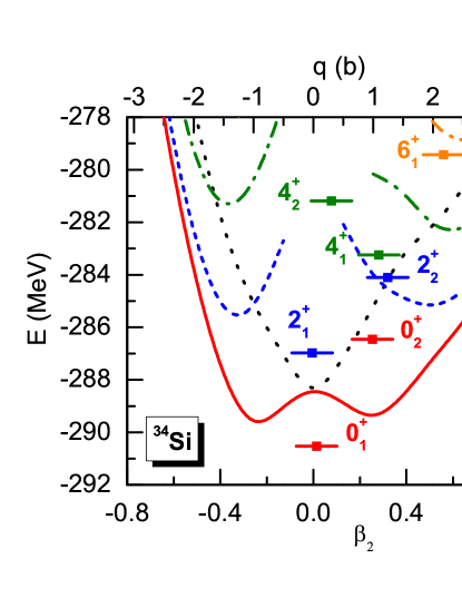
Figure 1: (Color online) Energy curves for the particle-number-projected HFB states (N&Z) and particle-number and angular-momentum projected states ($J=0$, 2, 4, 6 curves) for ${}^{34}\textrm{Si}$ as a function of the intrinsic quadrupole deformation of the mean-field states they are projected from. The solid square dots correspond to the lowest GCM solutions, which are plotted at their average deformation $\sum_{q}q\;|g_{\mu}^{J}(q)|^{2}$ (see text).

The energy curves obtained after projection on particle number and on angular momentum are shown in Fig. 1. The abscissa corresponds to the mass quadrupole moment $q$ of the intrinsic states that is projected (upper scale) and, equivalently, to the dimensionless quadrupole deformation

$$\beta_{2}=\sqrt{\frac{5}{16\pi}}\frac{4\pi}{3R^{2}A}\,\langle Q_{2}\rangle\,,$$ (8)

where $R=1.2\,A^{1/3}$ fm.

The particle-number-projected energy curve presents a spherical minimum with a steep rise with deformation (dotted line), as expected for a nucleus with large neutron and proton shell gaps, cf. Fig. 2. The projection on total angular momentum $J=0$ leads to energy curves with prolate and oblate minima at about the same deformation $|\beta_{2}|\approx 0.26$. The presence of these two minima is a usual result of angular-momentum projection when the non-projected energy curve presents a spherical minimum Bender06a ; Egido04 ; Bender08LH . In fact, at small deformation, the states of a given $J$ projected out from prolate and oblate mean-field states with the same $|\beta_{2}|$ value are almost equivalent. Oblate and prolate minima are also obtained for higher $J$-values. Our results are very similar to those of a similar calculation using the Gogny interaction Rod2000a .

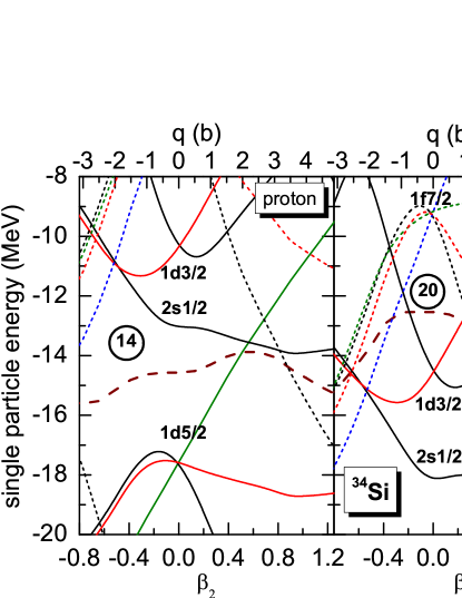
Figure 2: (Color online) Nilsson diagram of the eigenvalues of the single-particle Hamiltonian for neutrons (left panel) and protons (right panel) as obtained with the Skyrme interaction SLy4 for ${}^{34}\textrm{Si}$ as a function of the quadrupole deformation. Solid (dotted) lines represent levels of positive (negative) parity, and black, red, green and blue color represents levels with expectation values of $\langle j_{z}\rangle=1/2$, $3/2$, $5/2$ and $7/2$. The thick long-dashed line represents the Fermi energy. Single-particle levels are labeled for the spherical configuration only.

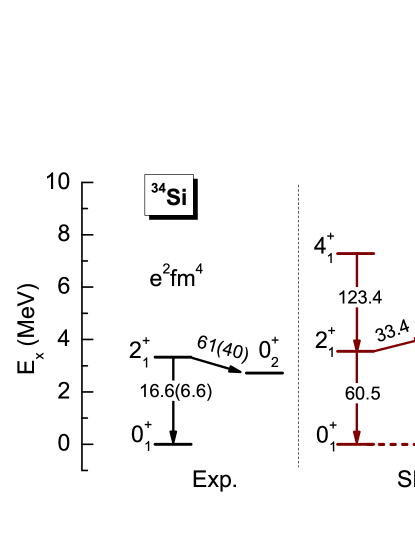
Figure 3: (Color online) Comparison between the experimental (left) and calculated (right) excitation energies $E_{x}$ and $B(E2)$ values (in units of $e^{2}$ fm⁴) for the low-lying states of ${}^{34}\textrm{Si}$. Experimental data are taken from Ref. Rotaru2011 .

The energies $E_{\mu}^{J}$ of the lowest GCM states are also shown in Fig. 1 (solid square with a label $J^{\pi}_{\mu}$) at the mean deformation $\sum_{q}q\;|g_{\mu}^{J}(q)|^{2}$ of the mean-field states on which they are build. This mean deformation is not an observable; still, it often provides a good indication about the dominating mean-field configurations in a GCM state. The mean deformations and the $B(E2)$ transition strengths suggest to organize the correlated states into the two structures displayed in Fig. 3, where the computed transition probabilities and the energy of the levels are also compared with the available experimental values Rotaru2011 . Our result can be interpreted as resulting from the coexistence of an anharmonic spherical vibrator and a prolate deformed band at low excitation energy. Both structures are not pure and distorted by their strong mixing.

The energy of the recently observed low-energy $0^{+}_{2}$ state Rotaru2011 and the out-of-band $B(E2:2^{+}_{1}\rightarrow 0^{+}_{2})$ value are reproduced rather well. However, the electric monopole $\rho^{2}(E0;0^{+}_{2}\rightarrow 0^{+}_{1})$ and the in-band $B(E2;2^{+}_{1}\rightarrow 0^{+}_{1})$ are overestimated by our model: $58.1\times 10^{-3}$ compared to the experimental value of $13.0\,(0.9)\times 10^{-3}$ Rotaru2011 for the former and 60.5 $e^{2}$ fm⁴ compared to 16.6 $e^{2}$ fm⁴ for the latter. This discrepancy might indicate Heyde88 that the two lowest $0^{+}$ GCM states are too strongly mixed in our calculation. The corresponding collective wave functions $g_{\mu}^{J}(q)$ are displayed in Fig. 4. Both are indeed spread over a very wide range of deformations, with similar contributions at small deformation $|\beta_{2}|\approx 0$. The ground state is peaked around the deformations of the two minima in the $J=0$ projected energy curve, cf. Fig. 1. By contrast,the wave function of the $0^{+}_{2}$ state is peaked at large prolate and oblate deformations where at least one downsloping level from the neutron $f_{7/2}$ shell becomes intruder by crossing the upsloping levels from the $sd$ shell, cf. Fig. 2. This is consistent with the interpretation of the $0^{+}_{2}$ state in ${}^{34}\textrm{Si}$ as a counterpart of the deformed ground state of the slightly lighter nuclei located in the so-called “island of inversion” Rotaru2011 .

IV Density distribution

Figure 4: (Color online) Collective wave functions $g_{\mu}^{J}(q)$ (cf. Eq. (6)) of the two lowest GCM solutions for $J=0$.

To quantify the depletion of the proton density distribution, we will use a depletion factor

$$F_{\text{max}}\equiv\frac{\rho_{\textrm{max},p}-\rho_{\textrm{cent},p}}{\rho_{\textrm{max},p}}\,,$$ (9)

which has been used in Ref. Chu2010 ; Grasso2009 and that measures the reduction of the density at the nucleus center relatively to its maximum value.

The effect of pairing correlations, projection on good quantum numbers and configuration mixing on the radial profiles of the proton, neutron and total densities is displayed in Fig. 5. The densities of the HF, HFB+LN and particle-number projected HFB+LN states are compared to those of the GCM $0^{+}$ ground state. To facilitate the comparison, the proton and neutron densities are rescaled by $A/Z$ and $A/N$ factors, respectively.

A large depletion at $r=0$ and a bulge at $r\approx 1.8$ fm are obtained for the proton density when the HF method is used (top left panel of Fig. 5). The HF neutron density, however, has an opposite behavior, with a flat shoulder at intermediate $r$ values and a bump at the nucleus center. This bump is similar to the one found experimentally for the charge density in ${}^{40}\textrm{Ca}$ Sick79 . Altogether, the total density has an almost flat, even slowly rising, profile in the interior of the nucleus. The same compensation of neutron and proton densities in the system’s interior is also found at all other stages of the calculation.

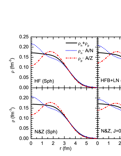
Figure 5: (Color online) Neutron, proton and total radial densities at $x=y=0$ for ${}^{34}\textrm{Si}$ for the spherical HF state (top left panel), the spherical HFB+LN state (top right) and its projection on good particle numbers ($N\&Z$, bottom left), as well as for the GCM $0^{+}_{1}$ ground state ($N\&Z$, $J=0$, GCM, bottom right). Neutron and proton densities have been rescaled with the factors $A/N$ and $A/Z$, respectively.

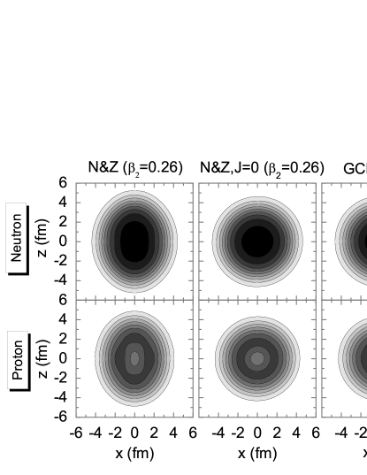
Figure 6: Contour plots of the neutron (upper panels) and proton (lower panels) densities in the $y=0$ plane for the particle number projected HFB+LN state with $\beta_{2}=0.26$ (left column), its projection on both particle numbers and total angular momentum $J=0$ (middle column) and for the $0^{+}$ GCM ground state (right column).

Unconstrained HFB calculations for ${}^{34}\textrm{Si}$ give the same result as the HF approximation. This is because the large $Z=14$ gap of about 4.5 MeV between the proton $1d_{5/2}$ and $2s_{1/2}$ levels in the single-particle spectrum prevents the protons from becoming superfluid at the HFB approximation. The even larger $N=20$ gap in the single-particle spectrum has the same effect for neutrons. The situation is different for nuclei such as ²²O and ⁴⁶Ar, where pairing correlations are already active at the HFB level and wash out the bubble structure predicted by HF calculations Grasso2009 .

The collapse of pairing correlations when the density of single-particle levels falls below a critical value is a deficiency of the HFB method Ring80 ; Rodriguez05 . It can be partially corrected by using the LN procedure (top right panel of Fig. 5). The level occupation is then smeared over the Fermi energy and the proton $2s_{1/2}$ orbital becomes partially occupied. As a consequence, the central proton density rises considerably from $F_{\text{max}}=0.41$ (HF) to $F_{\text{max}}=0.32$ (HFB+LN). The HFB+LN density presented in Fig. 5 is calculated using occupation numbers corrected for particle-number projection by the approximation described for example in Ref. Quentin90 . Using the non-corrected BCS occupation numbers instead would overestimate the effect of pairing and give a much larger reduction of the depletion factor.

Projection of the HFB+LN state on good particle numbers (bottom left panel of Fig. 5) substantially reduces the pairing correlations, and the density profiles almost go back to the HF ones with $F_{\text{max}}=0.36$. This reflects the well-known fact that the LN approximation overestimates the correlations in the weak pairing limit (whereas HFB underestimates them), cf. for example Ref. Anguiano02 , and indicates that in this case a correct treatment of pairing requires to go beyond the mean field.

The behavior of the density close to the origin is usually discussed in terms of the occupation of single-particle states in the spherical HF basis. This is not obvious in a method like the one that we use where the mean-field basis is different for each deformation. Deformation mixes single-particle states with different orbital angular momentum. In particular, when one expands a deformed basis in terms of the spherical one, the proton $2s_{1/2}$ level gets partially filled. The situation is even more complicated after projection and configuration mixing, cf. the bottom right panel of Fig. 5. We have seen in Fig. 4 that the collective wave function of the $0^{+}$ GCM ground state is spread over a wide range of intrinsic deformations.

Figure 6 illustrates how the density distribution of neutrons (upper panels) and protons (lower panels) is modified at different levels of our calculation. The left column shows contour plots of both densities for the particle-number projected HFB+LN state with $\beta_{2}=0.26$ that after angular-momentum projection gives the prolate minimum of the $J=0$ curve in Fig. 1. The proton density still exhibits a central depletion, but less pronounced than it is for the spherical HFB+LN state, reflecting the partial filling of the $2s_{1/2}$ level by deformation. After projection on total angular momentum $J=0$ (middle column), the density is obtained in the laboratory frame and is spherical. However, the central depression of the density is similar to the one found when projecting on particle numbers only. The configuration mixing leading to the GCM $0^{+}$ ground state (right column) increases the central proton density again and simultaneously reduces the value at the bulge, see the bottom right panel of Fig. 5, which in combination reduces the depletion factor to $F_{\text{max}}=0.21$. The values of central and maximum densities and of the depletion factor for the states discussed above are summarized in Table 1.

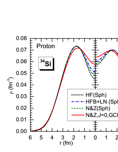
Figure 7: (Color online) Comparison of point-proton densities (left) with the folded charge densities (right) for ${}^{34}\textrm{Si}$ for the same states as in Fig. 5.

Up to now we have discussed the density of point protons and neutrons, thereby neglecting that protons and neutrons are composite particles of extended size. When searching for experimental signature of a depleted central density in ${}^{34}\textrm{Si}$ by elastic electron scattering, however, this has to be taken into account. The observable charge density is calculated by convolution of the proton density with a Gaussian form factor Negele70 with a proton size $a=\sqrt{2/3}\;\langle r^{2}\rangle^{1/2}_{p}=0.65$ fm, which for spherically symmetric density distributions leads to

$$\rho_{\rm ch}(r)=\frac{1}{a\sqrt{\pi}}\int\!dr^{\prime}r^{\prime}\,\rho_{p}(r^{\prime})\,\left[\frac{e^{-(r-r^{\prime})^{2}/a^{2}}}{r}-\frac{e^{-(r+r^{\prime})^{2}/a^{2}}}{r}\right]\,.$$ (10)

The charge density (right panel) is compared in Figure 7 to the point proton density (left panel) for the same four cases discussed in Fig. 5. Like correlations, the convolution (10) tends to even out the variations of the density profile: the central density rises and the maximum density of the outer bulge becomes smaller. In combination, both leads to a substantial reduction of the depletion factor from $F_{\text{max}}=0.41$ for the point proton density in a spherical HF calculation to $F_{\text{max}}=0.09$ for the charge density of the $0^{+}$ GCM ground state.

Adding correlations, the root-mean-square (rms) radius of the point proton density increases from 3.127 fm for the spherical HF state to 3.133 fm for the particle-number projected spherical HFB+LN state and to 3.180 fm for the GCM $0^{+}$ ground state. Looking at the density profiles in Fig. 7 the larger radius of the GCM $0^{+}$ ground state might appear counter-intuitive, as, at small radii $<3$ fm, the protons are obviously shifted to the inside. At larger radii, however, the tail of the density of the GCM $0^{+}$ ground state becomes slightly larger than the density of the other states, which is almost undetectable on the linear scale of Fig. 7. Because of the factor $r^{4}$ in the mean-square radius integral in polar coordinates, this tail is much more important than the center of the nucleus.

Figure. 7 puts into evidence that the reduction of the depletion factor at each stage of the calculation is partly due to the reduction of the maximum density $\rho_{\text{max}}$ Obviously, shell effects can reduce the density at some radii, but also enhance it at others. This indicates that the definition of the depletion factor (9) contains an ambiguity concerning the reference density. An alternative definition of a depletion factor could be

$$F_{\text{sat},\tau}\equiv\frac{\rho_{\textrm{sat},\tau}-\rho_{\textrm{cent},\tau}}{\rho_{\textrm{sat},\tau}}\,,$$ (11)

where $\rho_{\textrm{sat},\tau}$ with $\tau=p$, $n$, $t$ is now the saturation value of the proton, neutron, and total density. For ${}^{34}\textrm{Si}$, we have $\rho_{\text{sat},p}=(14/34)\times 0.16$ fm${}^{-3}=0.066$ fm^-3, $\rho_{\text{sat},n}=(20/34)\times 0.16$ fm${}^{-3}=0.094$ fm^-3, and $\rho_{\text{sat},t}=0.16$ fm^-3, respectively. Unlike $F_{\text{max}}$, this alternative depletion factor $F_{\text{sat}}$ can also be used to quantify central bumps in the density distribution.

Table 1: Central and maximum proton density of ${}^{34}\textrm{Si}$ and the depletion factors $F_{\text{max},p}$ [cf. Eq. (9)] and $F_{\text{sat},\tau}$ [cf. Eq. (11)]. For the latter, values for proton, neutron and the total densities are given. All densities are in fm^-3. The three first lines correspond to a spherical state. The values labeled with $N\&Z$, $J=0$ correspond to the prolate minimum of the $N\&Z$, $J=0$ projected energy curve of Fig. 1.

	$\rho_{\text{cent},p}$	$\rho_{\text{max},p}$	$F_{\text{max},p}$	$F_{\text{sat},p}$	$F_{\text{sat},n}$	$F_{\text{sat},t}$
HF	0.044	0.074	0.41	0.34	$-0.37$	$-0.08$
HFB+LN	0.050	0.074	0.32	0.24	$-0.31$	$-0.08$
$N$&$Z$	0.047	0.074	0.36	0.28	$-0.30$	$-0.06$
$N$&$Z$, $J=0$	0.051	0.073	0.30	0.22	$-0.27$	$-0.07$
GCM(g.s.)	0.057	0.073	0.21	0.13	$-0.22$	$-0.07$

Table 2: Same as Table 1, but for the charge density, Eq. (10).

	$\rho_{\text{cent}}$	$\rho_{\text{max}}$	$F_{\text{max}}$	$F_{\text{sat}}$
HF	0.056	0.071	0.21	0.15
HFB+LN	0.060	0.071	0.16	0.09
$N$&$Z$	0.058	0.071	0.18	0.12
$N$&$Z$, $J=0$	0.060	0.070	0.14	0.09
GCM(g.s.)	0.064	0.070	0.09	0.04

The results of Figs. 5 and 7 using these two depletion factors are summarized in Tables 1 and 2. The value of $\rho_{\textrm{sat},p}$ is systematically smaller than the values of $\rho_{\textrm{max},p}$ and, as a consequence, the values of $F_{\textrm{sat}}$ for protons are smaller than those of $F_{\text{max}}$. For neutrons, the value of $F_{\text{max},n}$ is always negative because of the central bump of the neutron density distribution. Again, the large central bump predicted by the HF calculation is reduced when correlations are added. Altogether, the central total density is always larger than saturation density as evidenced by $F_{\text{sat},t}$.

V Further discussion and conclusions

There are two major differences between the structure of ${}^{34}\textrm{Si}$ as predicted by our calculation and the structure of other candidates for bubble structure that have been discussed in the 1970s-1990s. First, as discussed above, the depletion of the central density in ${}^{34}\textrm{Si}$ appears for the proton density only, whereas the total density has an almost flat distribution throughout the bulk of the nucleus. Second, the level ordering of bubble nuclei is usually different from the one of regular nuclei, which is not the case for ${}^{34}\textrm{Si}$. Take, for example, the hypothetical bubble-type configuration of the ${}^{36}\textrm{Ar}$ discussed in Ref. Davies73 . There, the sequence of single-particle levels is altered such that the $2s_{1/2}$ level is pushed above the $1d_{3/2}$ level for both protons and neutrons. By contrast, for ${}^{34}\textrm{Si}$ only the relative distance of levels is changed such that the $Z=14$ gap opens up, cf. Fig. 2. In the absence of a bubble structure of the total density, and of the rearrangement of shells that is typical for bubble nuclei, the predicted anomaly of the proton density distribution of ${}^{34}\textrm{Si}$ appears to be an example of a central depression of the density, as observed also for many other nuclides Friedrich86 , rather than a nuclear bubble.

Taking into account correlations reduces the central depletion of the proton density in ${}^{34}\textrm{Si}$, as expected from earlier studies of other systems. Our main findings are:

1. A HFB+LN calculation overestimates proton pairing correlations in ${}^{34}\textrm{Si}$. Particle-number projection of the spherical state constructed with HFB+LN reduces the pairing correlations, such that the density profile almost goes back to the HF one. Clearly, a treatment of pairing correlations beyond the mean field with exact particle-number projection is needed in this case.

2. Fluctuations in quadrupole degrees of freedom strongly even out the fluctuations in the density profile; the central depression and the outer bump of the proton density are reduced, as is the central bump of the neutron density.

3. The central depletion of the density is less pronounced when looking at the experimentally observable charge density instead of the point proton density.

While all of the above findings can be expected to be generic on a qualitative level, the quantitative increase of the depletion factor when going from spherical HF to full projected GCM might depend on choices made for the effective interaction. In particular, in view of the somewhat too large mixing that we find between the two lowest $0^{+}$ GCM states, our calculation might slightly overestimate the role of shape fluctuations in the ground state.

As discussed in the introduction, a central depletion of the proton density of ${}^{34}\textrm{Si}$ has been suggested as an explanation for the reduction by about 0.6 MeV of the spin-orbit splitting of the neutron $3/2^{-}$ and $1/2^{-}$ levels inferred from transfer reactions Burgunder2011 ; Sorlin2011 . One has to be careful about such conclusion. First, the connection between the centroids of the spectral strength function of combined one-nucleon pick-up and removal reactions and the eigenvalues of the single-particle Hamiltonian is model-dependent Duguet11 , and when looking at the dominating fragments only, the comparison is far from clear. Second, as the symmetry-restored GCM method corresponds to a superposition of many states obtained with different mean fields, there is no straightforward procedure that would allow for a statement about effective single-particle energies based on the density profile from our calculation. The only meaningful way to compare with the data would be to perform the same kind of calculation for ³⁵Si and ³⁷S, which at present, however, is out of our reach.

When discussing the spin-orbit splitting of the neutron $2p$ levels in ${}^{34}\textrm{Si}$, there is an additional complication that goes even beyond these considerations. At spherical shape, the neutron $2p_{3/2}$ and $2p_{1/2}$ levels are far above the Fermi energy and outside of the energy interval shown in the Nilsson diagram of Fig. 2. In our spherical HF calculation of ${}^{34}\textrm{Si}$, the former is weakly bound at $-0.56$ MeV, whereas the latter is even unbound at $+0.83$ MeV. In such a situation, the coupling to the continuum has to be carefully taken into account, which is a task that goes beyond our study. By contrast, both single-particle levels are predicted to be (weakly) bound in a similar HF calculation for ${}^{36}\textrm{S}$.

In summary, we find that correlations from pairing and fluctuations in quadrupole deformation substantially reduce the central depletion of the proton density in ${}^{34}\textrm{Si}$. The extension of our method to the calculation of transition densities in the laboratory frame as observables in inelastic electron scattering is currently underway Yao2012 .

VI Acknowledgments

Fruitful discussions with Stephane Grévy, Witold Nazarewicz and Olivier Sorlin are gratefully acknowledged. This research was supported in parts by the PAI-P6-23 of the Belgian Office for Scientific Policy, the F.R.S.-FNRS (Belgium),by the European Union’s Seventh Framework Programme under grant agreement n 262010, the National Science Foundation of China under Grants No. 11105111 and No. 10947013, the Fundamental Research Funds for the Central Universities (XDJK2010B007), the Southwest University Initial Research Foundation Grant to Doctor (SWU109011), the French Agence Nationale de la Recherche under Grant No. ANR 2010 BLANC 0407 ”NESQ”, and by the CNRS/IN2P3 through the PICS No. 5994.

References

- (1) H. Überall, Electron Scattering from Complex Nuclei, Parts A and B (Academic Press, New York, 1971).
- (2) R. C. Barrett, Rep. Prog. Phys. 37, 1 (1974).
- (3) J. L. Friar and J. W. Negele, Adv. in Nucl. Phys. 8, 219 (1975).
- (4) I. Sick, in Advanced Methods in the Evaluation of Nuclear Scattering Data, Lecture Notes in Physics Vol. 236, 137 (1985).
- (5) J. Friedrich, N. Voegler, and P.-G. Reinhard, Nucl. Phys. A459, 10 (1986).
- (6) B. Frois and C. N. Papanicolas, Ann. Rev. Nucl. Part. Sci. 37, 133 (1987).
- (7) P. E. Hodgson, Hyperfine Interactions 74, 75 (1992).
- (8) F. J. Kline, H. Crannell, J. T. O’Brien, J. McCarthy, R. R. Whitney, Nucl. Phys. A209, 381 (1973).
- (9) D. Beck, A. Bernstein, I. Blomqvist, H. Caplan, D. Day, P. Demos, W. Dodge, G. Dodson, K. Dow, S. Dytman, M. Farkhondeh, J. Flanz, K. Giovanetti, R. Goloskie, E. Hallin, E. Knill, S. Kowalski, J. Lightbody, R. Lindgren, X. Maruyama, J. McCarthy, B. Quinn, G. Retzlaff, W. Sapp, C. Sargent, D. Skopik, I. The, D. Tieger, W. Turchinetz, T. Ueng, N. Videla, K. von Reden, R. Whitney, and C. Williamson, Phys. Rev. Lett. 59, 1537 (1987); ibid., 2388(E).
- (10) A. Amrouna, V. Bretona, J.-M. Cavedon, B. Frois, D. Goutte, F. P. Juster, Ph. Leconte, J. Martino, Y. Mizuno, X.-H. Phan, S. K. Platchkov, I. Sick, S. Williamson, Nucl. Phys. A579, 596 (1994).
- (11) M. Wakasugi, T. Suda and Y. Yano, Nucl. Instrum. Methods Phys. Res., Sect. A532, 216 (2004).
- (12) T. Suda and M. Wakasugi, Prog. Part. Nucl. Phys. 55, 417 (2005).
- (13) T. Suda, M. Wakasugi, T. Emoto, K. Ishii, S. Ito, K. Kurita, A. Kuwajima, A. Noda, T. Shirai, T. Tamae, H. Tongu, S. Wang, and Y. Yano, Phys. Rev. Lett. 102, 102501 (2009).
- (14) A. N. Antonov et al., Nucl. Instrum. Methods Phys. Res., Sect. A637, 60 (2011).
- (15) I. Sick, J. B. Bellicard, J. M. Cavedon, B. Frois, M. Huet, P. Leconte, P. X. Ho, S. Platchko, Phys. Lett. B88, 245 (1979).
- (16) M. Bender, P.-H. Heenen, and P.-G. Reinhard, Rev. Mod. Phys. 75, 121 (2003).
- (17) C. Y. Wong, Phys. Lett. B41, 451 (1972).
- (18) C. Y. Wong, Ann. Phys. (N.Y.) 77, 279 (1973).
- (19) K. T. R. Davies, C. Y. Wong, and S. J. Krieger, Phys. Lett. B41, 455 (1972).
- (20) K. T. R. Davies, S. J. Krieger and C. Y. Wong, Nucl. Phys. A216, 250 (1973).
- (21) M. Beiner and R. J. Lombard, Phys. Lett. B47, 399 (1973).
- (22) X. Campi and D. W. L. Sprung, Phys. Lett. B46, 291 (1973).
- (23) S. G. Nilsson, J. R. Nix, P. Möller, and I. Ragnarsson, Nucl. Phys. A222 (1974) 221.
- (24) G. Saunier, B. Rouben, and J. M. Pearson, Phys. Lett. B48, 293 (1974).
- (25) K. Dietrich and K. Pomorski, Nucl. Phys. A627, 175 (1997).
- (26) J. Dechargé, J.-F. Berger, K. Dietrich, and M. S. Weiss, Phys. Lett. B451, 275 (1999).
- (27) M. Bender, K. Rutz, P.-G. Reinhard, J. A. Maruhn, and W. Greiner, Phys. Rev. C 60, 034304 (1999).
- (28) J. Dechargé, J.-F. Berger, M. Girod, and K. Dietrich, Nucl. Phys. A716, 55 (2003).
- (29) W. Nazarewicz, M. Bender, S. Cwiok, P.-H. Heenen, A. Kruppa, P.-G. Reinhard, and T. Vertse, Nucl. Phys. A701, 165c (2002).
- (30) B. G. Todd-Rutel, J. Piekarewicz, and P. D. Cottle, Phys. Rev. C 69, 021301(R) (2004).
- (31) Y. Chu, Z. Ren, Z. Wang, and T. Dong, Phys. Rev. C 82, 024320 (2010).
- (32) E. Khan, M. Grasso, J. Margueron, and Nguyen Van Giai, Nucl. Phys. A800, 37 (2008).
- (33) M. Grasso, L. Gaudefroy, E. Khan, T. Niksic, J. Piekarewicz, O. Sorlin, Nguyen Van Giai, and D. Vretenar, Phys. Rev. C 79, 034318 (2009).
- (34) G. Burgunder, thèse, GANIL T 2011-06, Universtié de Caen, http://tel.archives-ouvertes.fr/tel-00695010 (2011).
- (35) O. Sorlin, private communication (2012).
- (36) L. Bennour, P.-H. Heenen, P. Bonche, J. Dobaczewski, and H. Flocard, Phys. Rev. C 40, 2834 (1989).
- (37) A. Faessler, S. Krewald, A. Plastino and J. Speth, Z. Phys. A 276, 91 (1976).
- (38) P.-G. Reinhard and S. Drechsel, Z. Phys. A 290, 85 (1979).
- (39) D. Gogny, in Nuclear Physics with Electromagnetic Interactions, H. Arenhövel and D. Drechsel [edts.], Lecture Notes in Physics, Vol. 108 (Springer-Verlag, New York, 1979), p. 88.
- (40) J. Dechargé, M. Girod, D. Gogny and B. Grammaticos, Nucl. Phys. A358, 203c (1983).
- (41) H. Esbensen and G. F. Bertsch, Phys. Rev. C 28, 355 (1983).
- (42) M. B. Johnson and G. Wenes, Phys. Rev. C 38, 386 (1988).
- (43) F. Barranco and R. A. Broglia, Phys. Rev. Lett. 59, 2724 (1987).
- (44) T. Sil and S. Shlomo, Phys. Scr. 78, 065202 (2008).
- (45) M. Girod and and D. Gogny, Phys. Lett. B64, 5 (1976).
- (46) M. Girod and P.-G. Reinhard, Nucl. Phys. A384, 179 (1982).
- (47) M. Bender, G. F. Bertsch, and P.-H. Heenen, Phys. Rev. C 73, 034322 (2006).
- (48) J. L. Egido and L. M. Robledo, in Extended Density Functionals in Nuclear Physics, G. A. Lalazissis, P. Ring, D. Vretenar [edts.], Lecture Notes Phys. 641 (Springer, Berlin, 2004), p. 269.
- (49) M. Bender, Eur. Phys. J. ST156, 217 (2008).
- (50) T. Nikšić, D. Vretenar, and P. Ring, Phys. Rev. C 74, 064309 (2006).
- (51) M. Bender and P.-H. Heenen, Phys. Rev. C 78, 024309 (2008).
- (52) T. R. Rodríguez and J. L. Egido, Phys. Rev. C 81, 064323 (2010).
- (53) J. M. Yao, J. Meng, P. Ring, and D. Vretenar, Phys. Rev. C 81, 044311 (2010).
- (54) P. Bonche, H. Flocard, and P.-H. Heenen, Comput. Phys. Commun. 171, 49 (2005).
- (55) P. Ring and P. Schuck, The Nuclear Many-Body Problem (Springer, Heidelberg, 1980).
- (56) D. Lacroix, T. Duguet, and M. Bender, Phys. Rev. C 79, 044318 (2009).
- (57) E. Chabanat, P. Bonche, P. Haensel, J. Meyer, and R. Schaeffer, Nucl. Phys. A635, 231 (1998); Nucl. Phys. A643, 441(E) (1998).
- (58) C. Rigollet, P. Bonche, H. Flocard, and P.-H. Heenen, Phys. Rev. C 59, 3120 (1999).
- (59) J. M. Yao, M. Bender, and P.-H. Heenen, (to be published).
- (60) R. Rodríguez-Guzmán, J.L. Egido and L.M. Robledo, Phys. Lett. B 474, 15 (2000).
- (61) F. Rotaru, F. Negoita, S. Grévy et al., (to be published).
- (62) K. Heyde and R. A. Meyer, Phys. Rev. C 37, 2170 (1988).
- (63) T. R. Rodríguez, J. L. Egido, and L. M. Robledo, Phys. Rev. C 72, 064303 (2005).
- (64) P. Quentin, N. Redon, J. Meyer, and M. Meyer, Phys. Rev. C 41, 341 (1990); ibid, 43, 361(E) (1991).
- (65) M. Anguiano, J. L. Egido, and L. M. Robledo, Phys. Lett. B545, 62 (2002).
- (66) J. W. Negele, Phys. Rev. C 1, 1260 (1970).
- (67) T. Duguet and G. Hagen, Phys. Rev. C 85, 034330 (2012) and references therein.