Coupled Intermittent Maps Modelling the Statistics of Genomic Sequences: A Network Approach

Abstract

The dynamics of coupled intermittent maps is used to model the correlated structure of genomic sequences. The use of intermittent maps, as opposed to other simple chaotic maps, is particularly suited for the production of long range correlation features which are observed in the genomic sequences of higher eucaryotes. A weighted network approach to symbolic sequences is introduced and it is shown that coupled intermittent polynomial maps produce degree and link size distributions with power law exponents similar to the ones observed in real genomes. The proposed network approach to symbolic sequences is generic and can be applied to any symbol sequence (artificial or natural).

I Introduction

Some 20 years ago, in 1992, the presence of long range correlations in genomic sequences was first reported in three seminal papers li:1992 ; peng:1992 ; voss:1992 . Since then many attempts were made to record, classify and model these genomic correlations and to connect them with the functionality and evolution of the current day genome li:1992 ; peng:1992 ; voss:1992 ; arneodo:2010 ; buldyrev:1995 ; herzel:1998 ; li:1994 ; katsaloulis:2006 ; messer:2007 . Despite these many attempts a conclusive explanation of the presence and the role of long range correlations in the genome is still missing.

In an earlier publication provata:2010 , one of the current authors (A.P.) and P. Katsaloulis have searched for a hierarchical process which could produce long range correlations similar to the ones observed in genomic sequences. To this end, they introduced a 2D density correlation matrix M which is based on the frequency of appearance of blocks/strings of size $s$. They calculated the multifractal properties of DNA from this matrix and from its multiple superpositions to create strings of longer lengths. In fact, their approach corresponds to a description of all strings of multiple lengths $2s,4s\cdots$, assuming that the correlations are negligible for length scales $l>s$. This method produces correlations up to finite scales, which are comparable with the ones observed in the genome at the same length scales provata:2010 . Nevertheless, long-range correlations are known to persist over many scales in DNA and are not limited to a finite length scale provata:2007 ; katsaloulis:2009 . In a further quest for dynamical mechanisms producing long range correlations over extended scales the current study uses the dynamics of intermittent maps to produce symbol sequences with characteristics similar to DNA.

Intermittent maps are well-known to produce a variety of interesting features such as metastable behaviour and anomalous transport, often characterised by long-term correlations and power laws dettmann:1998 ; balakrishnan:2001 ; korabel:2005 ; korabel:2007 ; pollicott:2009 ; froyland:2011 ; bhansali:2005 . That is why they are particularly suited for the modelling of the dynamics of DNA strands with long range features, such as the genome of higher eucaryotes. In particular, the polynomial mapbhansali:2007eco is particularly suited for the DNA modeling due to its simplicity, versatility and the large parameter range which gives rise to long range characteristics. This map will be used in the modeling of genomic data by first transforming the times series generated by the map into a symbol sequence and then comparing its statistics with that of whole eucaryotic chromosomes.

For the comparison between the dynamics produced by the intermittent polynomial map and that of genomic sequences a novel network approach will first be established. For this, the time series produced by the polynomial maps will be transformed into symbol sequences and then associated networks will be constructed. The properties of these networks (degree distribution, link size distribution, clustering coefficients) will be computed both for the polynomial map and for the genomic sequences and the statistics will be compared. It will turn out that the use of single polynomial maps is not enough to produce the exact power law exponents observed in the network description of the genome. The solution to this problem is given by weakly coupling the polynomial maps on a lattice. The weak coupling modifies the power law exponents of the zero-coupling limit and produces power law tails comparable to the ones observed for the genome data.

This work has the following structure: In the next section the dynamics of the intermittent polynomial map is briefly recapitulated and the corresponding symbol sequence is constructed. The construction of a dynamical weighted network method for the description of correlations in symbol sequences is presented in the same section. In Sec. III the network method is applied to both, human chromosomes and symbol sequence of the intermittent polynomial map. Comparative results are presented and discussed. In Sec. IV, coupled polynomial maps are discussed. It is shown that small couplings give exponents very close to the ones observed for genomic sequences. In our concluding remarks of section V the general use of the network method is summarized.

II Intermittent Maps and Associated Networks

In this section we first recall the dynamics of the polynomial map and describe the transformation to symbol sequence for later comparison with genomic sequences. It is important to note here that uniformly distributed symbol frequencies will not be assumed in the current study. The symbol frequency produced by the map will depend on the chosen partition of the phase space and will be dictated by comparison with real genomic sequences where the symbol frequencies have different average values for each symbol.

II.1 The Polynomial Map

The polynomial map is defined by the following iteration scheme bhansali:2007 ; bhansali:2005

$$x_{n+1}=\left\{\begin{array}[]{l l l}x_{n}(1+2^{\alpha}x_{n}^{\alpha}),&\quad{\rm if}&x_{n}\leq 0.5\\ 2x_{n},&\quad{\rm if}&x_{n}>0.5\\ \end{array}\right.\>\>n=1,2...$$ (3)

where $n$ is a discrete time index and $x_{n}\in[0,1]$ is taken modulo 1 for all $n$ and $\alpha>0$. For $0<\alpha<1$ the map is ergodic. Figure 1 shows the graph of $x_{n+1}$ vs. $x_{n}$ of the polynomial map for a parameter $\alpha=0.5$ located in the center of the ergodic regime.

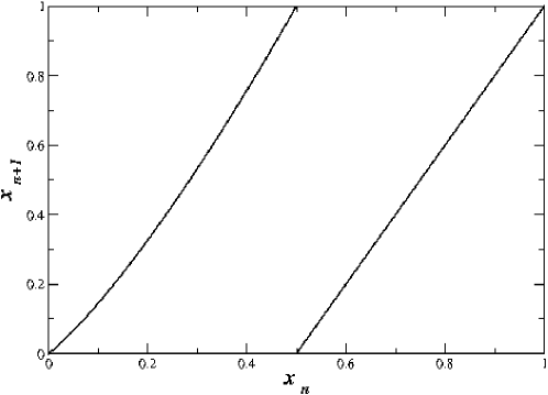
Figure 1: (Colour online) The polynomial map with parameter value $\alpha=0.5$.

Note that near $x_{n}\sim 0$ the slope is close to 1 and hence intermittent behavior is produced. In a symbolic dynamics approach, the laminar phase of intermittent behavior corresponds to repetitions of the same symbol for quite a long time, which is then interrupted by chaotic outbursts BS . The symbol repetitions generate long-term correlations. A similar feature is also observed in genomic sequences. For DNA very often particular substrings of symbols are repeated again and again, causing a dynamics that is significantly different from random behaviour and exhibiting long-term correlations. For this reason it is obvious that intermittent maps, as opposed to simple, fully developed chaotic maps, are good candidates to model sequences of symbols with similar statistics as in genomes.

II.2 Symbol Sequences Associated with Maps

The symbolic dynamics technique for the analysis of maps has a long tradition (see, e.g., BS for an introduction). The resulting sequences carry the correlations inherited by the map and provide the means of understanding the dynamical behavior in a coarse-grained way.

To comply with the structure of genomic sequences we use a translation based on $m=4$ symbols. The phase space is partitioned into four segments $[0,M_{1}),\>[M_{1},M_{2}),\>[M_{2},M_{3}),\>[M_{3},1]$, where $M_{i},\,i=1,2,3$ are real numbers, chosen in such a way that the frequency of appearance of the four nucleotides in a particular chromosome is reproduced by the map. Using this phase space partition the time series produced by Eq. 3 is transformed into a sequence $L=l_{1},l_{2},l_{3},\ldots$, with symbols taken from a 4-letter alphabet representing the four nucleotides: $l_{i}\in[A(Adenine),G(Guanine),C(Cytosine),T(Thymine)]$.

$$l_{i}=\left\{\begin{array}[]{l l l}A,&\quad{\rm if}&0\leq x_{i}<M_{1}\\ G,&\quad{\rm if}&M_{1}\leq x_{i}<M_{2}\\ C,&\quad{\rm if}&M_{2}\leq x_{i}<M_{3}\\ T,&\quad{\rm if}&M_{3}\leq x_{i}<1\end{array}\right.\>\>i=1,2...$$ (8)

As a particular example we consider Human Chromosome 20, where the individual nucleotide frequencies are: $p_{A}=0.282856,p_{C}=0.215134,p_{G}=0.215896$ and $p_{T}=0.286114$. To calculate the $M_{i}$ values, we first determine the invariant density of the polynomial map, i.e. we iterate the map and calculate the local density of points, or probability $p(x)$ that a specific value will occur between $x$ and $x+dx$. For this chromosome the $M_{i}$ $i=1,\cdots 4$, are determined as:

$$\begin{array}[]{l}\int_{0}^{M_{1}}p(x)dx=p_{A}=0.282856\\ \int_{M_{1}}^{M_{2}}p(x)dx=p_{G}=0.215896\\ \int_{M_{2}}^{M_{3}}p(x)dx=p_{C}=0.215134\end{array}$$ (12)

By using the transformation Eq. 8 of map Eq. 3 with $M_{j}$ values given by Eq. 12 an arbitrarily long symbol sequence $l_{i},i=1,\cdots,N$ is produced, whose correlations are dictated by the polynomial map and whose symbol frequencies correspond to the ones of chromosome 20.

II.3 Network Approach to Symbolic Sequences

In this section a general relation between networks and symbol sequences is established. This construction is generic and holds for any symbol sequence whether it is a natural or experimental symbol sequence (eg. natural languages, DNA) or an artificial sequence. In the second category random sequences are included, as well as sequences obtained via certain rules/algorithms and sequences obtained e.g. by map iteration processes, as described in the previous section.

Consider a generic symbolic sequence

$$L=l_{1},l_{2},\cdots l_{i}\cdots l_{N}$$ (13)

of length $N$, where the symbols $l_{i}$ take values from a finite alphabet of size $m$. For our approach the sequence $L$ is covered with (divided into) segments (blocks, strings) of size $s<<N$. The maximum number of all possible strings of size $s$ with symbols taken from an alphabet with $m$ symbols is

$$S_{max}=m^{s}$$ (14)

To fully cover the sequence, $N/s$ segments are needed . As a concrete example consider covering the binary ($m=2$) sequence $L=\{001010001101011011001\}$ by strings of size $s=3$. The following substrings occur: $S_{1}=\{001\},\>\>S_{2}=\{010\},\>\>S_{3}=\{101\},\>\>S_{4}=\{011\}$ with string $S_{1}$ occurring three times and string $S_{4}$ occurring twice.

In uncorrelated, random sequences of infinite size all strings $S_{i},\>\>i=1,\cdots S_{max}$ of length $s$ occur with the same probability

$$p_{i}=1/S_{max},\>\>i=1,\cdots S_{max}$$ (15)

while for correlated and natural sequences Eq. 15 usually does not hold. In natural and correlated sequences the total number of observed strings is denoted by $V$ and is always $V\leq S_{max}$.

Within the ensembles of possible $S_{i}$ consider furthermore the probability $b_{ij}$ of string $i=[I_{1},I_{2}\cdots I_{s}]$ to be followed by string $j=[J_{1},J_{2}\cdots J_{s}]$ (both having the same length $s$). The elements $b_{ij}$ are identified actually as conditional probabilities: having located the string $i$ in the sequence $L$, the element $b_{ij}$ represents the conditional probability that it is followed by the string $j$. $\mathbf{b}$ is a square matrix of size $V\times V$. The matrix $\mathbf{b}$ can be related to the joint probability of finding the combined string $i\otimes j=[I_{1},I_{2}\cdots I_{s},J_{1},J_{2}\cdots J_{s}]$ of length $2s$ as follows:

$$b_{ij}=\frac{p_{i\otimes j}}{p_{i}}=\frac{p_{[I_{1},I_{2}\cdots I_{s},J_{1},J_{2}\cdots J_{s}]}}{p_{[I_{1},\cdots,I_{s}]}}$$ (16)

Based on the conditional probability $b_{ij}$ of string $i$ to be followed by string $j$ on a very long sequence $L$, an associated, abstract network can be constructed whose nodes are the strings $S_{i},\>\>i=1,\cdots V$ of length $s$. Thus the number of nodes, or network capacity $V$, is at most $S_{max}$. An edge is drawn between two nodes $i$ and $j$ if the corresponding strings $i=[I_{1},I_{2}\cdots I_{s}]$ and $j=[J_{1},J_{2}\cdots J_{s}]$ are found in direct succession anywhere in the sequence $L$. The edge between $i$ and $j$ nodes is weighted with the frequency of finding strings $i$ and $j$ in succession and thus the conditional probability matrix element $b_{ij}$ gives the weight of the edge between nodes $i$ and $j$. In the network notation the matrix $b_{ij}$ is identified as the connectivity or adjacency matrix. Note that in general $b_{ij}\neq b_{ji}$ for genomic or natural symbolic sequences. Thus the adjacency matrix created by genomic sequences indicates that the corresponding network belongs to the class of directed networks/graphs.

In the abstract networks generated by symbolic sequences as proposed above, loops (sometimes also called ”self-loops” or ”buckles”) are often present, since it is quite common that a certain string will be followed by an identical string. Loops do not occur in social networks, for example, where an individual does not interact with himself. On the other hand, in food distribution networks between cities self-loops on nodes are allowed, since food maybe consumed (or distributed) in the city it was produced. Loops are also observed in genomic networks, brain neuron networks, cardio-vascular system etc. kivela:2004 ; makitie:1999 ; ahn:2009 ; dojer:2006 . In terms of the elements of the connectivity matrix, the presence of loops means $b_{ii}\neq 0$. In graph theory, graphs which contain loops are often called multigraphs.

Having defined the nodes and links in the network corresponding to a symbol sequence we proceed in identifying the various network parameters. The degree $k_{i}$ of a node $i$, which corresponds to the symbolic string $i=[I_{1},I_{2},\cdots I_{s}]$, is usually defined as the number of links originating from the node $i$ towards any other node in the system. For weighted networks, as in the case of symbol sequences, each link is weighted with the appropriate weighting factor and the degree $k_{i}$ expresses the cumulative weighted linking of the particular node $i$ to all other network nodes. In the case of symbol sequences, (where the links are identified as the conditional probabilities $b_{ij}$), the outflowing degree $k_{i}$ of string $i$ is calculated as

$$k_{i}=\sum_{j=1}^{V}b_{ij}=\frac{\sum_{j=1}^{V}p_{i\otimes j}}{p_{i}}=1$$ (17)

Thus, when we use the conditional probability $b_{ij}$, all nodes carry the same outflowing degree (normalized to 1), since each string is always followed by another string within the $V$ possible strings. However, since we are dealing with directed networks, we also have to take into account the inflowing degrees of freedom. The probability to observe a certain string $i$ is then given by the balance between inflow and outflow.

In the case of symbol sequences we identify the degree $k_{i}$ of a node $i$ as the frequency of appearance of the corresponding string $i$, to be consistent with the distributed weights carried by the nodes . This definition makes sense: For dynamical systems with a Markov partition the invariant probabilities of string sequences are determined by the balance between inflowing and outflowing iterates (a direct consequence of the fixed-point property of the Perron-Frobenius operator). Hence the net balance of flow along the links fixes the invariant density and hence also the probabilities of symbol sequences in a coarse-grained description.

The distribution of nodes which carry degree $k$ is denoted by $P(k)$. This means we now look at the set of all observed frequencies of symbol sequences, and consider the probability distribution of these frequencies. For example, if all symbol sequence probabilities are the same, as for example for uncorrelated random sequences of infinite length, then $P(k)$ corresponds to a sharply peaked delta distribution. The quantity $P(k)$ is called the degree distribution. It characterizes the network globally and classifies it to be a scale-free network if $P(k)$ has power law tails,

$$P(k)\sim k^{-\gamma}.$$ (18)

$\gamma$ is the power law exponent expressing the scale-free nature of the network and it is typically in the range $2<\gamma<3$, although in some cases $\gamma$ may lie outside this interval.

Apart from the degree distribution, one of the most important variables in the theory of complex networks is the local clustering coefficient $c_{n}$ around the node $n$, which describes the local structure of the network around that specific node. The local clustering coefficient is defined as:

$$c_{n}=\frac{\sum_{i,j}b_{ni}b_{ij}b_{jn}}{\sum_{i\neq j}b_{ni}b_{jn}}$$ (19)

In Eq. 19 the numerator is related to the total weighted number of closed triangles originating from node $n$, while the denominator gives the maximum number of possible triangles originating on the same node grindrod:2002 ; saramaki:2007 . Sometimes it is possible to find the functional form of the clustering coefficient $c(k)$ of nodes having degree $k$. This is an important property of the network and indicates an underlying hierarchical structure ravasz:2003 . For hierarchical networks a power law form is achieved

$$c(k)\sim k^{-b}$$ (20)

where the exponent $b$ takes a positive value for hierarchical networks, while it is constant for random uncorrelated networks and for scale free networks. In many natural networks $b\sim 1$ ravasz:2003 . In general it is difficult to find such a relation. It is important here to make the distinction between $c(k)$, which is the functional form of the clustering coefficient as a function of the degree $k$, and $c_{i}$ which is the clustering coefficient of node $i$.

The global clustering coefficient $c(V)$, defined as the average of the local clustering ones, characterises globally the connectivity in the network and in general depends on the size $V$ of the network.

$$c(V)=<c_{i}>=\frac{1}{V}\sum_{i=1}^{V}c_{i}.$$ (21)

For many real systems $c(V)$ is independent of $V$. In particular, the global clustering coefficient in random uncorrelated networks decreases as watts:1998

$$c(V)\sim V^{-1}.$$ (22)

In the case of scale-free, highly clustered and complex networks Eq. 22 changes to

$$c(V)\sim V^{-\nu}.$$ (23)

The distribution of clustering coefficients $P(c)$ takes a power law form in scale free networks,

$$P(c)\sim c^{-\beta}.$$ (24)

For random, uncorrelated networks, it was shown by Watts and Strogatz that the local clustering coefficients have an exponential type of distribution watts:1998 ; ravasz:2003 .

In view of the presence of self-loops in genomic sequences, their contributions in the node degrees and the clustering coefficients need to be commented on. In the numerator of Eq. 19 the presence of the term $b_{kk}b_{kk}b_{kk}$ might seem strange in social networks but in the representation of symbolic sequence it represents the phenomenon of repeats, i.e. the repetition of the same string a number of times in the sequence. If the node $j$ represents the string $j\equiv[J_{1},J_{2},\cdots J_{s}]$, where $J_{i}$ are symbols, then the term $b_{jj}b_{jj}b_{jj}$ denotes the presence of string $j\otimes j\otimes j\otimes j$ in the sequence. Repetitions are very frequent in genomic sequences, in particular for primates. In the human genome one sequence repeat alone (the ALU-sequence) comprises approximately 11.5% of the human genome, while the total repeat content reaches 35% of the human DNA.

III Network Properties of DNA Sequences and of Intermittent Maps

III.1 DNA sequences

In this section we first apply the network approach to genomic sequences, following the ideas described in the previous section. As working examples we use chromosomes 10, 14 and 20 from the human genome.

In natural sequences such as in DNA most often $b_{ij}\neq b_{ji}$. In genomic sequences the two strands of the helix have complimentary structure. Let us call the two strands $C1$ and $C2$. This means that if a nucleotide A is found in a certain position in $C1$ a nucleotide $T$ will be found in the sequence $C2$ in the same position. Similarly, $T$ is the compliment of $A$, $C$ is the compliment of $G$ and $G$ is the compliment of $C$. Consider e.g. the string $S_{1}=[AGGT]$ followed by $S^{\prime}_{1}=[CGTT]$ both found in strand $C1$. Then in strand $C2$, the following strings will be found: $S_{2}=[TCCA]$ and $S^{\prime}_{2}=[GCAA]$. Thus if we denote by $\>\>\>\tilde{}\>\>\>$ the complimentary strings and strands, we have the following relation for the weighting matrices,

$$b_{ij}(s)=\tilde{b}_{\tilde{i}\tilde{j}}(s)$$ (25)

It is then sufficient to compute the network characteristics of one of the two strands and to mirror its properties to the other strand according to Eq. 25.

In Fig. 2a the degree distribution of the symbolic network characterising the chromosome 20 genomic sequence of Homo sapiens is presented. Strings of different sizes were considered, up to $s=9$. In the $x-$axis the degree $k$ characterising the total link strength carried by a node is plotted, normalised with the total number of (weighted) links. This normalisation is needed because the total number of links is a decreasing function of the length $L$ of the symbol sequence. The $y-$axis shows the distribution of nodes of degree $k$. For comparison, the dashed line represents a pure power law distribution with exponent $\gamma=-3$.

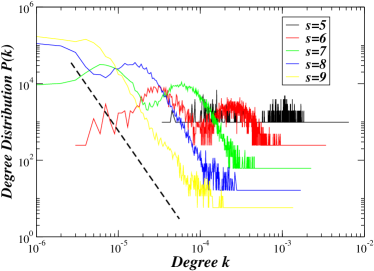
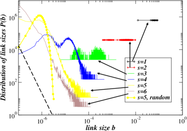
Figure 2: (Colour online) Distribution functions related to the network derived from the Human chromosome 20. a)The Degree Distribution $P(k)$ of the network of strings with various sizes $s$. The dashed line corresponds to a power law decay with exponent $\gamma\sim-3$. b) The Distribution $P(b)$ of link weights $b_{ij}$ between nodes. The dashed line corresponds to an exact power law with exponent $\gamma_{1}=-3$. The yellow bullets correspond to a random and uncorrelated sequence with $s=5$. Strings of various sizes s are plotted with different colours as indicated in the figure.

In Fig. 2b the distribution of individual link sizes (weights $b_{ij}$) is plotted independently of the node to which they belong. String sizes $s=1-6$ are shown, taken also for the human chromosome 20. Longer string sizes are not possible to investigate due to computational limitations, since the size of the matrix $\mathbf{b}$ grows exponentially with $s$. The observed form of the $P(b)$ distribution is very similar to that of $P(k)$ in Fig. 2a. This is not unexpected since the values in the latter figure represent cumulative link weights originating from one node. Again the dashed line corresponds to power law behaviour with exponent $\gamma_{1}=-3$. The two exponents may not be exactly identical, due partly to stochasticity and partly to the fact that the degree is a sum over a finite number of link sizes (over a node). If the number of links on a node were infinite then the two distributions would posses exactly the same exponent $\gamma\equiv\gamma_{1}$. For comparison, the $P(b)$ distribution calculated from a random and uncorrelated symbol sequence of the same size as chromosome 20 is plotted with yellow bullets. The segmentation was done with $s=5$. In contrast to the genomic data, the random symbol sequence shows a hump around the mean value $5\times 10^{-7}$ and then drops abruptly (step-like), as is expected for finite, uncorrelated random sequences.

Note that for the case of symbol sequences the degree of a node coincides with the frequency of appearance of the particular string of length $s$. For $s=1$ (one-letter words) there are only 4 configurations and all of them have similar frequency. That results in a narrow range distribution with little structure. For $s=2$ (two-letter words) a first appearance of two maxima is observed, which correspond to the presence of multiple $T$ and $A$ in the sequence. The minimum values correspond to the infrequent presence of the complex $GC$ in the system, which is known to be related to the presence of functional units called promoters. For $2<s<6$ the presence of a larger number of strings/nodes in the network smoothes the two well-pronounced maxima into a two-humped distribution. Again, the two maxima correspond to the presence of multiple $A$ and $T$ strings, while the minimum is again corresponding to the complexes of $GC$ and $CG$ followed by one of the other four bps. For $s>5$ a power law degree distribution establishes gradually, which indicates the scale free character of this symbolic network.

For comparison, the degree distributions as computed for human chromosomes 10, 14 and 20 are plotted together in Fig. 3. The degree distributions of the three chromosomes are qualitatively similar, which may point to a universal type of scaling. In the same figure the degree distribution of a random sequence of the same size as chromosome 20 is plotted. The random distribution is single-humped and is symmetric around its mean value, as expected for random uncorrelated sequences. Clearly, for infinitely long random sequences one expects convergence to a $\delta$-function, whereas for genomic sequences the distribution is much broader.

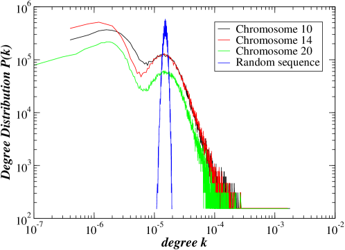
Figure 3: (Colour online) The degree distributions for 3 different human chromosomes. The degree distribution of a random symbol sequence of the same size is also shown (humped distribution).

To further explore the network connectivity we compute the size distribution of clustering coefficients, throughout the network. Due to computer memory limitations only strings of size $s\leq 6$ can be computed. To suppress fluctuations, the cumulative size distribution $P_{cum}(c)$ is calculated as

$$P_{cum}(C)=\int_{C}^{\infty}P(c)dc.$$ (26)

For power law distributions of the form 24, the cumulative size distribution also follows a similar power law, as

$$P_{cum}(C)\sim\int_{C}^{\infty}c^{-\beta}dc\sim C^{-\beta+1}.$$ (27)

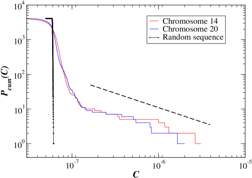
Figure 4: (Colour online) The cumulative distribution of clustering coefficients $P_{cum}(c)$ is plotted as a function of the size $c$ for human chromosomes 14 (red line), 20 (blue line) and a random sequence (black line) of equal size with chromosome 20. String size is $s=6$. For comparison the dashed line presents a pure power law decay with exponent $-1.7$.

In Fig. 4 the cumulative clustering coefficient distribution is plotted as a function of the coefficient size $C$. Data from chromosomes 20 and 14 are plotted together with data taken from an artificial random symbol sequence whose symbol frequencies are the same as in chromosome 20. In a double logarithmic scale the genomic cumulative distributions exhibit an almost linear regime for large sizes, indicating the presence of a power law. This behavior becomes more prominent as the string size increases. In comparison, the data from the large-length random sequence has an abrupt, almost step-like decay, indicating a very sharply peaked Gaussian ($\delta$-like) distribution, whose cumulative distribution function is very close to a step-like function.

III.2 Polynomial map

Methods to construct networks from maps or a given time series have been previously addressed in refs. nicolis:2005 ; net1 ; net2 ; robledo , using as a particular examples the tent map, the cusp map, or the logistic map. In nicolis:2005 , the phase space of the maps is segmented into a number of cells and each cell corresponds to a node of the network. The connectivity matrix is then defined by the frequency of transitions between the different cells/nodes of the network.

The current approach is inspired by nicolis:2005 , but the transition from the map to the network is achieved using symbolic sequence generated by the map. In other words, the map dynamics is first mirrored on a symbol sequence as explained in sec. II.2 and then the network is constructed from the symbol sequence as discussed in sec. II.3. The choice of the polynomial map, mentioned briefly in sec. II.1, is based on its intermittent behaviour and its capacity to give rise to time series (and corresponding symbol sequences) with long range features, as opposed to the dynamics of the logistic map and other non-intermittent maps giving rise to nearly uncorrelated behavior.

In Fig. 5a the cumulative degree distribution for the polynomial map is shown for various values of string sizes $s$ and parameter value $\alpha=0.5$. The sequence size was chosen as $L=4.3\cdot 10^{7}$, of comparable size as chromosome 20. In our plots we have chosen the cumulative degree distribution rather than the probability density function to somewhat smoothen out fluctuations. The frequency of appearance of each nucleotide is chosen as in Eq. 12 and corresponds to those of human chromosome 20. For this particular parameter value, all string sizes point towards the same exponent $\gamma(a=0.5)\sim 3$. Note that the number of allowed string configurations $V$ generated by the polynomial map is far less than the number of strings observed in human genomic sequences. As an example we note that $V_{DNA}(s=9)=244925<4^{9}=262144$, while $V_{poly}(s=9)=1790$.

In Fig. 5b the cumulative degree distribution for the polynomial map is shown for various values of the parameter value $\alpha$ and string sizes $s=9$. It is obvious that the exponent $\gamma$ is a decreasing function of the parameter $\alpha$. By appropriate choice of the value of $\alpha$ we can achieve the same power law exponent as the one observed in the human chromosome. On the other hand, the number of configurations generated by the polynomial map ($\sim 1700$) is far less than observed in genomic sequences ($\sim 250000$ in chromosome 20). This difference is non-trivial, it covers 2 orders of magnitude. To achieve the diversity of the string configurations together with the degree distribution scaling observed in genomic sequences, a diffusive coupling is introduced in the next section between a large number of polynomial maps (considered as ”units”). This will create a large variety of string configurations together with similar exponents as for genomic networks.

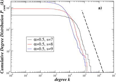
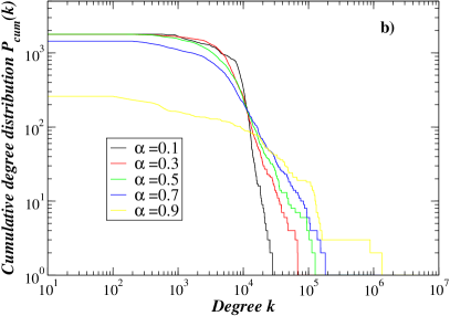
Figure 5: (Colour online) Network symbol representation of the polynomial map. a) Cumulative degree distribution for parameter value $\alpha=0.5$ and various string sizes. The dashed line corresponds to an exact power law with exponent $\gamma=-3$. b) Cumulative degree distribution for string size $s=9$ and various parameter values.

IV Network Properties of Coupled Polynomial Maps

Coupled Map Lattices (CML) have been extensively used for the modelling of many physical systems which involve interactions between many spatially separated constituents. A lot of emphasis of research activity has been put on spatio-temporal chaos and synchronization phenomena arising in CMLs kaneko:1984 ; kapral:1985 ; kaneko:1993 ; brannstrom:2005 ; lin:2002 ; schmitzer:2009 ; provata-beck:2011 .

For the coupling of polynomial maps, in the present study, a simple, 1-dimensional chain arrangement with periodic boundary conditions is assumed. The periodic boundary conditions are chosen simply for convenience and they do not affect, qualitatively or quantitatively, the results in the limit of very long chains, as considered here.

Our linear chain arrangement consists of $L=10^{8}$ polynomial maps coupled to their nearest neighbours with a coupling constant $r$. The dynamics is

$$x_{n+1}^{i}=\left\{\begin{array}[]{l l l}(1-r)x_{n}^{i}(1+2^{\alpha}(x_{n}^{i})^{\alpha})+\frac{1}{2}r\left[x_{n}^{i+1}(1+2^{\alpha}(x_{n}^{i+1})^{\alpha})+x_{n}^{i-1}(1+2^{\alpha}(x_{n}^{i-1})^{\alpha})\right]&\quad{\rm if}&x_{n}\leq 0.5\\ (1-r)2x_{n}+\frac{1}{2}r\left[2x_{n}^{i+1}+2x_{n}^{i-1}\right]&\quad{\rm if}&x_{n}>0.5\\ \end{array}\right.$$ (30)

The values $x^{i}_{n}$ are taken modulo 1 for all $n$, as in Eq. 3. The index $i=1,2\cdots$ runs over all local maps, while $n=1,2,\cdots$ is a temporal index. Random initial conditions are chosen for each map. The parameter value is chosen as $\alpha=0.5$ and the number of iterations in our simulation is $T=5000$, sufficiently high for the maps to enter their dynamic equilibrium regime. At $T=5000$ the state of each map is recorded and a transformation to a symbol sequence is performed using Eq. 12, with the same 1-point symbol sequences as for the chromosome data. At the final stage the symbol sequence is divided into strings of size $s$ and the corresponding network connectivity matrix $\mathbf{b}$ is constructed according to the method described in Sec. II.3.

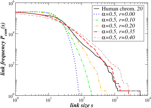
Figure 6: (Colour online) Coupled polynomial maps on a linear chain. The Cumulative Degree Distribution $P_{cum}(k)$ of the network is plotted for various values of the coupling constant $r$. For comparison the corresponding data for chromosome 20 are plotted with the black solid line. Parameter values are $\alpha=0.5,\>\>T=5000,\>\>L=4.3\>10^{7},\>\>s=9$. The symbol frequencies were chosen as in Eq. 12. Various values of the coupling constant $r$ are plotted, as indicated in the legend.

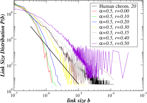
Figure 7: (Colour online) Coupled polynomial maps on a linear chain: The Link Size Distributions $P(b)$ of link weights $b_{ij}$ between all the nodes is plotted for various values of the coupling $r$. The data of chromosome 20 are represented by the black solid line. Parameter values are $\alpha=0.5,\>\>T=5000,\>\>L=4.3\cdot 10^{7},\>\>s=6$. The symbol frequencies were chosen as in Eq. 12. Results for various coupling rates $r$ are shown. The solid straight line represents an exact power law with exponent -3.

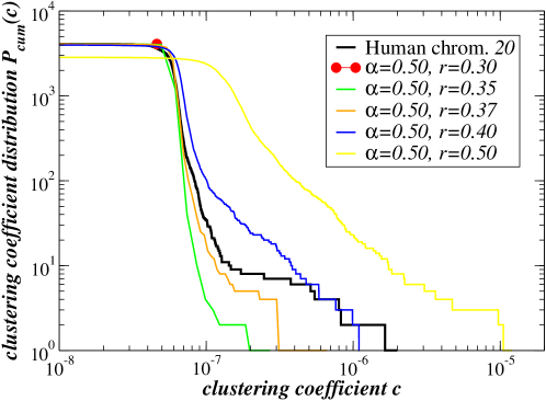
Figure 8: (Colour online) The cumulative distribution of clustering coefficients $P_{cum}(c)$ is plotted for various values of the coupling $r$. For comparison the data of chromosome 20 are plotted as a black solid line. All parameters (including nucleotide frequencies) are chosen as in Fig. 7.

In Figs. 6, 7 and 8 the cumulative degree distribution $P_{cum}(k)$, the link size distribution $P(b)$, and the cumulative distribution of clustering coefficients $P_{cum}(c)$ are plotted for various values of the coupling constant $r$. For comparison, the corresponding data for chromosome 20 are also plotted in each figure.

For the calculation of the degree distribution window size $s=9$ is used. In Fig. 6 the cumulative distribution is plotted. Comparison of the different curves reveals that the coupled polynomial maps with parameter $\alpha=0.5$ and coupling constant of the order of $r\sim 0.35$ assimilate relatively well the sequence structure of Chromosome 20.

For the calculation of the link size distribution strings of size $s=6$ were employed. This is because transition matrices of size $4^{s}\times 4^{s}$ need to be considered which are very demanding in computer memory. The results for $s=6$ are plotted in Fig. 7 both for Human Chromosome 20 (black solid line) and coupled polynomial maps with parameter $\alpha=0.5$ and various values of the coupling constant $r$. Again the best fit is observed for $r\sim 0.35$ despite the fact of using a different (smaller) string size $s$ for the calculations. This shows that the similarities between the statistics of chromosomes and coupled polynomial maps are robust to variations in the size of window used in the creation of the network, provided that $s$ is not too small ($s>5$). The observed power law exponent is again of the order $\sim 3$, as represented by the straight line in the double logarithmic scale in Fig. 7.

Finally, the distributions of clustering coefficients are presented in Fig. 8. Again, the genomic data (Chromosome 20) are plotted together with sequences resulting from coupled polynomial maps with $\alpha=0.5$ and various coupling rates $r$. The results are consistent with the previous findings. While for small values of $r$ the distribution of clustering coefficients drops abruptly as in random sequences, as $r$ grows the distribution develops a long tail which approaches the tails of DNA sequences around the coupling values $r\sim 0.35-0.40$.

We notice that uncoupled polynomial maps can not well represent the complexity of DNA sequences, although they are known to produce intermittency with long range correlations. On the other hand, a medium size coupling between polynomial maps is able to create the appropriate correlations and to resemble the structure of DNA in many levels of complexity. From the last three figures one can see that a coupling constant of the order of $r=0.35$ is enough to adjust the power law exponents to values close to the ones observed in genomic sequences. The need for a coupling between neighboring units to properly assimilate DNA sequences demonstrates the presence of local interactions between the adjacent nucleotide strings which create the correlated, mosaic structure of the genome.

Similar conclusions are obtained from the network analysis of other chromosomes. Just slight variations in the values of the exponents and the necessary coupling constants are noted due to the difference in the symbol frequencies in the chromosomes and due to stochastic effects.

From our analysis we also see that quite generally coupled polynomial maps give rise to complex small-world networks, via the corresponding symbol sequences and transition matrix, while the network exponents can be adjusted by varying the coupling constant $r$.

V Conclusions

The dynamics of coupled intermittent maps was used to model the correlated structure of genomic sequences via a network approach. The weighted network approach to symbolic sequence was first introduced and applied to genomic and random, uncorrelated sequences and then compared with the corresponding statistics of coupled intermittent maps. For the modelling the use of intermittent maps appears to be necessary in order to retrieve the scaling properties observed in the primary structure of DNA. It was first shown that although the dynamics of single intermittent maps produce long range correlated symbolic sequences, with a variety of power law exponents depending on the choice of the parameters, they do not produce the diversity of genomic strings observed in DNA sequences. To overcome this limitation coupled map lattices were considered, with diffusive coupling between neighboring units on a 1-dimensional lattice. It was shown that a medium size coupling between neighboring polynomial maps is sufficient to produce a) power law exponents comparable with the ones obtained from genomic data and b) a statistical distribution of string frequencies similar to real DNA sequences. Our results are consistent with the known existence of complicated patterns of correlations between adjacent segments in DNA.

The reported results concern the primary structure of human chromosomes. The network method can be applied to any genomic sequence provided it is long enough to assure reasonable statistics. It would be of great interest to study further classes of organisms with this method and explore the range of values of the network exponents for different organisms. Additionally, the proposed network approach to symbol sequences may be used to construct quite generally networks from any symbol sequence (natural, experimental or artificial) and to test for scaling characteristics.

References

- (1) W. Li and K. Kaneko, Europhysics Letters, 17, 655-660, (1992).
- (2) C.-K. Peng, S. V. Buldyrev, A. L. Goldberger, et al., Nature, 356, no. 6365, 168-170, (1992).
- (3) F. Voss, Fractals, 2, 1-6, (1992).
- (4) A. Arneodo, C. Vaillant, B. Audit, F. Argoul, Y. d’Aubenton-Carafa, C. Thermes, Physics Reports, 498, 45-188,(2010) (and references therein).
- (5) S. V. Buldyrev, A. L. Goldberger, S. Havlin, et al., Physical Review E, 51, 5084-5091, (1995).
- (6) H. Herzel, E. N. Trifonov, O. Weiss, and I. Grosse, Physica A, 249, 449-459, (1998).
- (7) W. Li, T. G. Marr, K. Kaneko, Physica D: Nonlinear Phenomena, 75, 392-416 (1994).
- (8) P. Katsaloulis, T. Theoharis, W.M. Zheng, B.L. Hao, A. Bountis, Y. Almirantis, A. Provata, Physica A, 366, 308-322, (2006).
- (9) P.W. Messer, J Comput Biol 14, 655-68 (2007).
- (10) A. Provata and P. Katsaloulis, Phys. Rev. E, 81, 026102 (2010).
- (11) A. Provata and T. Oikonomou, Phys. Rev. E, 75, 056102, (2007).
- (12) P. Katsaloulis, T. Theoharis and A. Provata, J. Theor. Biol. 258, 18-26, (2009).
- (13) C. P. Dettmann and P. Dahlqvist, Phys. Rev. E, 57, 5303-5310 (1998).
- (14) V. Balakrishnan, G. Nicolis and C. Nicolis, Stochastics and Dynamics (SD), 1, 345-359 (2001).
- (15) N. Korabel, A.V. Chechkin, R. Klages, I.M. Sokolov and V.Y. Gonchar, Europhys. Lett. 70, 63-69 (2005).
- (16) N. Korabel, R. Klages, A.V. Chechkin, I.M. Sokolov and V.Y. Gonchar, Phys. Rev. E 75, 036213 (2007).
- (17) M. Pollicott and R. Sharp, Nonlinearity 22 Number 9, 2079 (2009).
- (18) G. Froyland, R. Murray and O. Stancevic, Nonlinearity, 24 2435 (2011).
- (19) R.J. Bhansali, M. P. Holland and P. S. Kokoszka, Fields Inst. Comm. 44, 99-126, (2005).
- (20) R.J. Bhansali, M. P. Holland and P. S. Kokoszka, Intermittency, long memory and financial returns, Long Memory in Economics, pages 39-68 (2007).
- (21) R.J. Bhansali and M. P. Holland, Statistica Sinica, 17, 15-41 (2007).
- (22) C. Beck and F. Schlögl, Thermodynamics of Chaotic Systems, Cambridge University Press (1993).
- (23) T. Kivela, T. Makitie, R. T. Al-Jamal; P. Toivonen, Can. J. Ophthalmol., 39, 409-21 (2004).
- (24) T. Makitie, P. Summanen, A. Tarkkanen, T. Kivela, JNCI J Natl Cancer Inst, 91, 359-367 (1999).
- (25) S. Ahn, R. T. Wang, C. C. Park, A. Lin, R. M. Leahy, K. Lange, D. J. Smith, PloS Computational Biology, 5, e1000407 (2009).
- (26) N. Dojer, A. Gambin, A. Mizera, B. Wilczynski and J. Tiuryn, BMC Bioinformatics, 7, 249 (2006).
- (27) P. Grindrod, Phys. Rev. E, 66, 066702 (2002).
- (28) J. Saramaki, M. Kivela, J. -P. Onnela, K. Kaski and J. Kertesz, Phys. Rev. E, 75, 027105 (2007).
- (29) E. Ravasz and A. -L. Barabasi, Phys. Rev. E, 67, 026112 (2003).
- (30) D. J. Watts and S. H. Strogatz, Nature, 393 440-442 (1998).
- (31) G. Nicolis, A. Garcia Cantu and C. Nicolis, Bifurcation and Chaos, 15, 3467-3480 (2005).
- (32) J. Zhang and M. Small, Phys. Rev. Lett. 96, 238701 (2006).
- (33) Z. Gao and N. Jin, Chaos 19, 033137 (2009).
- (34) B. Luque et al., Chaos 22, 013109 (2012).
- (35) K. Kaneko, Progr. Theor. Phys, 72, 480 (1984).
- (36) R. Kapral, Phys. Rev. A, 31, 3868 (1985).
- (37) K. Kaneko (ed.) Theory and Applications of Coupled Map Lattices, Wiley, New York, 1993.
- (38) A. Brannstrom and D. J. T. Sumpter, Bull. Math. Biol. 67, 663-682 (2005).
- (39) W. -W. Lin and Y. -Q. Wang, SIAM J. Appl. Dyn. Syst. 1, 175-189 (2002).
- (40) B. Schmitzer, W. Kinzel and I. Kanter, Phys. Rev. E, 80, 047203 (2009).
- (41) A. Provata and C. Beck, Phys. Rev. E 83, 066210 (2011).