A Generalized Kernel Approach to Structured Output Learning

Abstract

We study the problem of structured output learning from a regression perspective. We first provide a general formulation of the kernel dependency estimation (KDE) approach to this problem using operator-valued kernels. Our formulation overcomes the two main limitations of the original KDE approach, namely the decoupling between outputs in the image space and the inability to use a joint feature space. We then propose a covariance-based operator-valued kernel that allows us to take into account the structure of the kernel feature space. This kernel operates on the output space and only encodes the interactions between the outputs without any reference to the input space. To address this issue, we introduce a variant of our KDE method based on the conditional covariance operator that in addition to the correlation between the outputs takes into account the effects of the input variables. Finally, we evaluate the performance of our KDE approach on three structured output problems, and compare it to the state-of-the-art kernel-based structured output regression methods.

1 Introduction

In many practical problems such as statistical machine translation (Wang & Shawe-Taylor, 2010) and speech recognition or synthesis (Cortes et al., 2005), we are faced with the task of learning a mapping between objects of different nature that each can be characterized by complex data structures. Therefore, designing algorithms that are sensitive enough to detect structural dependencies among these complex data is becoming increasingly important. While classical learning algorithms can be easily extended to complex inputs, more refined and sophisticated algorithms are needed to handle complex outputs. In this case, several mathematical and methodological difficulties arise and these difficulties increase with the complexity of the output space. Complex output data can be divided into three classes: 1) Euclidean: vectors or real-valued functions; 2) mildly non-Euclidean: points on manifolds and shapes; and 3) strongly non-Euclidean: structured data like trees and graphs. The focus in the machine learning and statistics communities has been mainly on multi-task learning (vector outputs) and functional data analysis (functional outputs) (Caruana, 1997; Ramsay & Silverman, 2005), where in both cases output data reside in a Euclidean space, but there has also been considerable interest in expanding general learning algorithms to structured outputs.

Table 1: This table summarizes the notations used in the paper.

input space	$\mathcal{X}$	structured output space	$\mathcal{Y}$
input data	$x_{i}\in\mathcal{X}$	structured output data	$y_{i}\in\mathcal{Y}$
scalar-valued kernel	$k:\mathcal{X}\times\mathcal{X}\rightarrow\mathbb{R}$	scalar-valued kernel	$l:\mathcal{Y}\times\mathcal{Y}\rightarrow\mathbb{R}$
output feature space	$\mathcal{F_{Y}}$	output feature map	$\Phi_{l}:\mathcal{Y}\rightarrow\mathcal{F_{Y}}$
set of operators on $\mathcal{F_{Y}}$ to $\mathcal{F_{Y}}$	$\mathcal{L(F_{Y})}$	operator-valued kernel	$K:\mathcal{X}\times\mathcal{X}\rightarrow\mathcal{L(F_{Y})}$
joint feature space	$\mathcal{F_{XY}}$	joint feature map	$\Phi_{K}:\mathcal{X}\times\mathcal{F_{Y}}\rightarrow\mathcal{F_{XY}}$
a mapping from $\mathcal{X}$ to $\mathcal{Y}$	$f$	a mapping from $\mathcal{X}$ to $\mathcal{F_{Y}}$	$g$

One difficulty encountered when working with structured data is that usual Euclidean methodology cannot be applied in this case. Reproducing kernels provide an elegant way to overcome this problem. Defining a suitable kernel on the structured data allows to encapsulate the structural information in a kernel function and transform the problem to a Euclidean space. Two different, but closely related, kernel-based approaches for structured output learning can be found in the literature (Bakir et al., 2007): kernel dependency estimation (KDE) and joint kernel maps (JKM). KDE is a regression-based approach that was first proposed by Weston et al. (2003) and then reformulated by Cortes et al. (2005). The idea is to define a kernel on the output space $\mathcal{Y}$ to project the structured output to a real-valued reproducing kernel Hilbert space (RKHS) $\mathcal{F_{Y}}$, and then perform a scalar-valued kernel ridge regression (KRR) between the input space $\mathcal{X}$ and the feature space $\mathcal{F_{Y}}$. Having the regression coefficients, the prediction is obtained by computing the pre-image from $\mathcal{F_{Y}}$. On the other hand, the JKM approach is based on joint kernels, which are nonlinear similarity measures between input-output pairs (Tsochantaridis et al., 2005; Weston et al., 2007). While in KDE separate kernels are used to project input and output data to two (possibly different) feature spaces, the joint kernel in JKM maps them into a single feature space, which then allows us to take advantage of our prior knowledge on both input-output and output correlations. However, this improvement requires an exhaustive pre-image computation during training, a problem that is encountered by KDE only in the test phase. Avoiding this computation during training is an important advantage of KDE over JKM methods.

In this paper, we focus on the KDE approach to structured output learning. The main contributions of this paper can be summarized as follows: 1) Building on the works of Caponnetto & De Vito (2007) and Brouard et al. (2011), we propose a more general KDE formulation (prediction and pre-image steps) based on operator-valued (multi-task) kernels instead of scalar-valued ones used by the existing methods (Sec. 3). This extension allows KDE to capture the dependencies between the outputs as well as between the input and output variables, which is an improvement over the existing KDE methods that fail to take into account these dependencies. 2) We also propose a variant (generalization) of the kernel trick to cope with the technical difficulties encountered when working with operator-valued kernels (Sec. 3). This allows us to (i) formulate the pre-image problem using only kernel functions (not feature maps that cannot be computed explicitly), and (ii) avoid the computation of the inner product between feature maps after being modified with an operator whose role is to capture the structure of complex objects. 3) We then introduce a novel family of operator-valued kernels, based on covariance operators on RKHSs, that allows us to take full advantage of our KDE formulation. These kernels offer a simple and powerful way to address the main limitations of the original KDE formulation, namely the decoupling between outputs in the image space and the inability to use a joint feature space (Sec. 4). 4) We show how the pre-image problem, in the case of covariance and conditional covariance operator-valued kernels, can be expressed only in terms of input and output Gram matrices, and provide a low rank approximation to efficiently compute it (Sec. 4). 5) Finally, we empirically evaluate the performance of our proposed KDE approach and show its effectiveness on three structured output prediction problems involving numeric and non-numerical outputs (Sec. 6). It should be noted that generalizing KDE using operator-valued kernels was first proposed in Brouard et al. (2011). The authors have applied this generalization to the problem of link prediction which did not require a pre-image step. Based on this work, we discuss both the regression and pre-image steps of operator-valued KDE, propose new covariance-based operator-valued kernels and show how they can be implemented efficiently.

2 Preliminaries

In this section, we first introduce the notations used throughout the paper, lay out the setting of the problem studied in the paper, and provide a high-level description of our approach to this problem. Then before reporting our KDE formulation, we provide a brief overview of operator-valued kernels and their associated RKHSs. To assist the reading, we list the notations used in the paper in Table 1.

2.1 Problem Setting and Notations

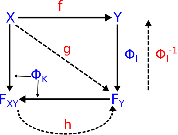
Given $(x_{i},y_{i})_{i=1}^{n}\in\mathcal{X}\times\mathcal{Y}$, where $\mathcal{X}$ and $\mathcal{Y}$ are the input and structured output spaces, we consider the problem of learning a mapping $f$ from $\mathcal{X}$ to $\mathcal{Y}$. The idea of KDE is to embed the output data using a mapping $\Phi_{l}$ between the structured output space $\mathcal{Y}$ and a Euclidean feature space $\mathcal{F_{Y}}$ defined by a scalar-valued kernel $l$. Instead of learning $f$ in order to predict an output $y$ for an input $x$, the KDE methods first learn the mapping $g$ from $\mathcal{X}$ to $\mathcal{F_{Y}}$, and then compute the pre-image of $g(x)$ by the inverse mapping of $\Phi_{l}$, i.e., $y=f(x)=\Phi_{l}^{-1}\big{(}g(x)\big{)}$ (see Fig. 1). All existing KDE methods use ridge regression with a scalar-valued kernel $k$ on $\mathcal{X}\times\mathcal{X}$ to learn the mapping $g$. This approach has the drawback of not taking into account the dependencies between the data in the feature space $\mathcal{F_{Y}}$. The variables in $\mathcal{F_{Y}}$ can be highly correlated, since they are the projection of $y_{i}$’s using the mapping $\Phi_{l}$, and taking this correlation into account is essential to retain and exploit the structure of the outputs. To overcome this problem, our KDE approach uses an operator-valued (multi-task) kernel to encode the relationship between the output components, and learns $g$ in the vector-valued (function-valued) RKHS built by this kernel using operator-valued kernel-based regression. The advantage of our formulation is that it allows vector-valued regression to be performed by directly optimizing over a Hilbert space of vector-valued functions, instead of solving independent scalar-valued regressions. As shown in Fig. 1, the feature space induced by an operator-valued kernel, $\mathcal{F_{XY}}$, is a joint feature space that contains information of both input space $\mathcal{X}$ and output feature space $\mathcal{F_{Y}}$. This allows KDE to exploit both the output and input-output correlations. The operator-valued kernel implicitly induces a metric on the joint space of inputs and output features, and then provides a powerful way to devise suitable metrics on the output features, which can be changed depending on the inputs. In this sense, our proposed method is a natural way to incorporate prior knowledge about the structure of the output feature space while taking into account the inputs.

Figure 1: Kernel Dependency Estimation. Our generalized formulation consists of learning the mapping $g$ using an operator-valued kernel ridge regression rather than a scalar-valued one as in the formulations of Weston et al. (2003) and Cortes et al. (2005). Using an operator-valued kernel mapping, we construct a joint feature space from information of input and output spaces in which input-output and output correlations can be taken into account.

2.2 Operator-valued Kernels and Associated RKHSs

We now provide a few definitions related to operator-valued kernels and their associated RKHSs that are used in the paper (see (Micchelli & Pontil, 2005; Caponnetto et al., 2008; Álvarez et al., 2012) for more details). These kernel spaces have recently received more attention, since they are suitable for leaning in problems where the outputs are vectors (as in multi-task learning (Evgeniou et al., 2005)) or functions (as in functional regression (Kadri et al., 2010)) instead of scalars. Also, it has been shown recently that these spaces are appropriate for learning conditional mean embeddings (Grunewalder et al., 2012). Let $\mathcal{L(F_{Y})}$ be the set of bounded operators from $\mathcal{F_{Y}}$ to $\mathcal{F_{Y}}$.

Definition 1

(Non-negative $\mathcal{L(F_{Y})}$-valued kernel) A non-negative $\mathcal{L(F_{Y})}$-valued kernel $K$ is an operator-valued function on $\mathcal{X}\times\mathcal{X}$, i.e., $K:\mathcal{X}\times\mathcal{X}\rightarrow\mathcal{L(F_{Y})}$, such that:

1. $\forall x_{i},x_{j}\in\mathcal{X},\;K(x_{i},x_{j})=K(x_{j},x_{i})^{*}$ ($*$ denotes the adjoint),

2. $\forall m\in\mathbb{N}_{+}^{*},\;\forall x_{1},\ldots,x_{m}\in\mathcal{X},\;\forall\varphi_{i},\varphi_{j}\in\mathcal{F_{Y}}\\ \sum\limits_{i,j=1}^{m}\langle K(x_{i},x_{j})\varphi_{j},\varphi_{i}\rangle_{\mathcal{F_{Y}}}\geq 0$.

The above properties guarantee that the operator-valued kernel matrix $\mathbf{K}=\big{[}K(x_{i},x_{j})\in\mathcal{L(F_{Y})}\big{]}_{i,j=1}^{n}$ is positive definite. Given a non-negative $\mathcal{L(F_{Y})}$-valued kernel $K$ on $\mathcal{X}\times\mathcal{X}$, there exists a unique RKHS of $\mathcal{F_{Y}}$-valued functions whose reproducing kernel is $K$.

Definition 2

($\mathcal{F_{Y}}$-valued RKHS) A RKHS $\mathcal{F_{XY}}$ of $\mathcal{F_{Y}}$-valued functions $g:\mathcal{X}\rightarrow\mathcal{F_{Y}}$ is a Hilbert space such that there is a non-negative $\mathcal{L(F_{Y})}$-valued kernel $K$ with the following properties:

1. $\forall x\in\mathcal{X},\;\forall\varphi\in\mathcal{F_{Y}}\hskip 36.135ptK(x,\cdot)\varphi\in\mathcal{F_{XY}}$,

2. $\forall g\in\mathcal{F_{XY}},\;\forall x\in\mathcal{X},\;\forall\varphi\in\mathcal{F_{Y}}\\ \langle g,K(x,\cdot)\varphi\rangle_{\mathcal{F_{XY}}}=\langle g(x),\varphi\rangle_{\mathcal{F_{Y}}}$.

Every RKHS $\mathcal{F_{XY}}$ of $\mathcal{F_{Y}}$-valued functions is associated with a unique non-negative $\mathcal{L(F_{Y})}$-valued kernel $K$, called the reproducing kernel.

3 Operator-valued Kernel Formulation of Kernel Dependency Estimation

In this section, we describe our operator-valued KDE formulation in which the feature spaces associated to input and output kernels can be infinite dimensional, contrary to Cortes et al. (2005) that only considers finite feature spaces. Operator-valued KDE is performed in two steps:

Step 1 (kernel ridge) Regression: We use operator-valued kernel-based regression and learn the function $g$ in the $\mathcal{F_{Y}}$-valued RKHS $\mathcal{F_{XY}}$ from the training data $\big{(}x_{i},\Phi_{l}(y_{i})\big{)}_{i=1}^{n}\in\mathcal{X}\times\mathcal{F_{Y}}$, where $\Phi_{l}$ is the mapping from the structured output space $\mathcal{Y}$ to the scalar-valued RKHS $\mathcal{F_{Y}}$. Similar to other KDE formulations, we consider the following regression problem:

$$\operatorname*{arg\,min}\limits_{g\in\mathcal{F_{XY}}}\sum\limits_{i=1}^{n}\|g(x_{i})-\Phi_{l}(y_{i})\|_{\mathcal{F_{Y}}}^{2}+\lambda\|g\|^{2},$$ (1)

where $\lambda>0$ is a regularization parameter. Using the representer theorem in the vector-valued setting (Micchelli & Pontil, 2005), the solution of (1) has the following form:

$$g(\cdot)=\sum\limits_{i=1}^{n}K(\cdot,x_{i})\psi_{i}\;,$$ (2)

where $\psi_{i}\in\mathcal{F_{Y}}$. Using (2), we obtain an analytic solution for the optimization problem (1) as

$$\mathbf{\Psi}=(\mathbf{K}+\lambda I)^{-1}\mathbf{\Phi_{l}}\;,$$ (3)

where $\mathbf{\Phi_{l}}$ is the column vector of $\big{[}\Phi_{l}(y_{i})\in\mathcal{F_{Y}}\big{]}_{i=1}^{n}$. Eq. 3 is a generalization of the scalar-valued kernel ridge regression solution to vector or functional outputs (Caponnetto & De Vito, 2007), in which the kernel matrix is a block operator matrix. Note that features $\Phi_{l}(y_{i})$ in this equation can be explicit or implicit. We show in the following that even with implicit features, we are able to formulate the structured output prediction problem in terms of explicit quantities that are computable via input and output kernels.

Step 2 (pre-image) Prediction: In order to compute the structured prediction $f(x)$ for an input $x$, we solve the following pre-image problem:

$$f(x) =\operatorname*{arg\,min}\limits_{y\in\mathcal{Y}}\|g(x)-\Phi_{l}(y)\|_{\mathcal{F_{Y}}}^{2}$$

$$=\operatorname*{arg\,min}\limits_{y\in\mathcal{Y}}\|\sum\limits_{i=1}^{n}K(x_{i},x)\psi_{i}-\Phi_{l}(y)\|_{\mathcal{F_{Y}}}^{2}$$

$$=\operatorname*{arg\,min}\limits_{y\in\mathcal{Y}}\|\mathbf{K}_{x}\mathbf{\Psi}-\Phi_{l}(y)\|_{\mathcal{F_{Y}}}^{2}$$

$$=\operatorname*{arg\,min}\limits_{y\in\mathcal{Y}}\|\mathbf{K}_{x}(\mathbf{K}+\lambda I)^{-1}\mathbf{\Phi_{l}}-\Phi_{l}(y)\|_{\mathcal{F_{Y}}}^{2}$$

$$=\operatorname*{arg\,min}\limits_{y\in\mathcal{Y}}\;l(y,y)-2\langle\mathbf{K}_{x}(\mathbf{K}+\lambda I)^{-1}\mathbf{\Phi_{l}},\Phi_{l}(y)\rangle_{\mathcal{F_{Y}}}$$

where $\mathbf{K}_{x}$ is the row vector of operators corresponding to input $x$. In many problems, the kernel map $\Phi_{l}$ is unknown and only implicitly defined through the kernel $l$. In these problems, the above operator-valued kernel formulation has an inherent difficulty in expressing the pre-image problem and the usual kernel trick is not sufficient to solve it. To overcome this problem, we introduce the following variant (generalization) of the kernel trick: $\langle\mathcal{T}\Phi_{l}(y_{1}),\Phi_{l}(y_{2})\rangle_{\mathcal{F_{Y}}}=[\mathcal{T}l(y_{1},\cdot)](y_{2})$, where $\mathcal{T}$ is an operator in $\mathcal{L(F_{Y})}$. Note that the usual kernel trick $\langle\Phi_{l}(y_{1}),\Phi_{l}(y_{2})\rangle_{\mathcal{F_{Y}}}=l(y_{1},y_{2})$ is recovered from this variant when $\mathcal{T}$ is the identity operator. It is easy to check that our proposed trick holds if we consider the feature space associated to the kernel $l$, i.e., $\Phi_{l}(y)=l(y,.)$. A proof for the more general case in which the features $\Phi_{l}$ can be any implicit mapping of a Mercer kernel is given for self-adjoint operator $\mathcal{T}$ in (Kadri et al., 2012, Appendix A). Using this trick, we may now express $f(x)$ using only kernel functions:

$$f(x)=\operatorname*{arg\,min}\limits_{y\in\mathcal{Y}}\;l(y,y)-2\big{[}\mathbf{K}_{x}(\mathbf{K}+\lambda I)^{-1}\mathbf{L}_{\bullet}\big{]}(y),$$ (4)

where $\mathbf{L}_{\bullet}$ is the column vector whose $i$’th component is $l(y_{i},\cdot)$. Note that the KDE regression and prediction steps of Cortes et al. (2005) can be recovered from Eqs. 3 and 4 using an operator-valued kernel $K$ of the form $K(x_{i},x_{j})=k(x_{i},x_{j})\mathcal{I}$, in which $k$ is a scalar-valued kernel and $\mathcal{I}$ is the identity operator in $\mathcal{F_{Y}}$.

Now that we have a general formulation of KDE, we turn our attention to build operator-valued kernels that can take into account the structure of the kernel feature space $\mathcal{F_{Y}}$ as well as input-output and output correlations. This is described in the next section.

4 Covariance-based Operator-valued Kernels

In this section, we study the problem of designing operator-valued kernels suitable for structured outputs in the KDE formulation. This is quite important in order to take full advantage of the operator-valued KDE formulation. The main purpose of using the operator-valued kernel formulation is to take into account the dependencies between the variables $\Phi_{l}(y_{i})$, i.e., the projection of $y_{i}$ in the feature space $\mathcal{F_{Y}}$, with the objective of capturing the structure of the output data encapsulated in $\Phi_{l}(y_{i})$. Operator-valued kernels have been studied more in the context of multi-task learning, where the output is assumed to be in $\mathbb{R}^{d}$ with $d$ the number of tasks (Evgeniou et al., 2005). Some work has also been focused on extending these kernels to the domain of functional data analysis to deal with the problem of regression with functional responses, where outputs are considered to be in the $L^{2}$-space (Kadri et al., 2010). However, the operator-valued Kernels used in these contexts for discrete (vector) or continuous (functional) outputs cannot be used in our formulation. This is because in our case the feature space $\mathcal{F_{Y}}$ can be known only implicitly by the output kernel $l$, and depending on $l$, $\mathcal{F_{Y}}$ can be finite or infinite dimensional. Therefore, we focus our attention to operators that act on scalar-valued RKHSs. Covariance operators on RKHS have recently received considerable attention. These operators that provide the simplest measure of dependency have been successfully applied to the problem of dimensionality reduction (Fukumizu et al., 2004), and played an important role in dealing with a number of statistical test problems (Gretton et al., 2005). We use the following covariance-based operator-valued kernel in our KDE formulation:

$$K(x_{i},x_{j})=k(x_{i},x_{j})C_{YY},$$ (5)

where $k$ is a scalar-valued kernel and $C_{YY}:\mathcal{F_{Y}}\rightarrow\mathcal{F_{Y}}$ is the covariance operator defined for a random variable $Y$ on $\mathcal{Y}$ as $\langle\varphi_{i},C_{YY}\varphi_{j}\rangle_{\mathcal{F_{Y}}}=\mathbb{E}\big{[}\varphi_{i}(Y)\varphi_{j}(Y)\big{]}$. The empirical covariance operator $\widehat{C}_{YY}^{(n)}$ is given by

$$\widehat{C}_{YY}^{(n)}=\frac{1}{n}\sum\limits_{i=1}^{n}l(\cdot,y_{i})\otimes l(\cdot,y_{i}),$$ (6)

where $\otimes$ is the tensor product $(\varphi_{1}\otimes\varphi_{2})h=\langle\varphi_{2},h\rangle\varphi_{1}$. The operator-valued kernel (5) is nonnegative since

$$\sum\limits_{i,j=1}^{m}\langle K(x_{i},x_{j})\varphi_{j},\varphi_{i}\rangle_{\mathcal{F_{Y}}}=\sum\limits_{i,j}^{m}\langle k(x_{i},x_{j})\widehat{C}_{YY}^{(n)}\varphi_{j},\varphi_{i}\rangle$$

$$=\sum\limits_{p=1}^{n}\sum\limits_{i,j}^{m}\frac{1}{n}\langle l(.,y_{p}),\varphi_{i}\rangle k(x_{i},x_{j})\langle l(.,y_{p}),\varphi_{j}\rangle\geq 0.$$

The last step is due to the positive definiteness of $k$.

The kernel (5) is a separable operator-valued kernel since it operates on the output space, and then encodes the interactions between the outputs, without any reference to the input space. Although this property can be restrictive in specifying input-output correlations, because of its simplicity, most of the operator-valued kernels proposed in the literature belong to this category (see (Álvarez et al., 2012) for a review of separable and beyond separable operator-valued kernels). To address this issue, we propose a variant of the kernel in (5) based on the conditional covariance operator,

$$K(x_{i},x_{j})=k(x_{i},x_{j})C_{YY|X},$$ (7)

where $C_{YY|X}=C_{YY}-C_{YX}C_{XX}^{-1}C_{XY}$ is the conditional covariance operator on $\mathcal{F_{Y}}$. This operator allows the operator-valued kernel to simultaneously encode the correlations between the outputs and to take into account (non-parametrically) the effects of the inputs. In Proposition 1, we show how the pre-image problem (4) can be formulated using the covariance-based operator-valued kernels in (5) and (7), and expressed in terms of input and output Gram matrices. The proof is reported in (Kadri et al., 2012, Appendix B).

Proposition 1

The pre-image problem of Eq. 4 can be written for covariance and conditional covariance operator-valued kernels defined by Eqs. (5) and (7) as

$$\operatorname*{arg\,min}\limits_{y\in\mathcal{Y}}\;l(y,y)-2\mathbf{L}_{y}^{\top}(\mathbf{k}_{x}^{\top}\otimes\mathbf{T})(\mathbf{k}\otimes\mathbf{T}+n\lambda I_{n^{2}})^{-1}\operatorname{vec}(I_{n}),$$ (8)

where $\mathbf{T}=\mathbf{L}$ for the covariance operator and $\mathbf{T}=\mathbf{L}-(\mathbf{k}+n\epsilon I_{n})^{-1}\mathbf{k}\mathbf{L}$ for the conditional covariance operator in which $\epsilon$ is a regularization parameter required for the operator inversion, $\mathbf{k}$ and $\mathbf{L}$ are Gram matrices associated to the scalar-valued kernels $k$ and $l$, $\mathbf{k}_{x}$ and $\mathbf{L}_{y}$ are the column vectors $\big{(}k(x,x_{1}),\ldots,k(x,x_{n})\big{)}^{\top}$ and $\big{(}l(y,y_{1}),\ldots,l(y,y_{n})\big{)}^{\top}$, $\operatorname{vec}$ is the vector operator such that $\operatorname{vec}(A)$ is the vector of columns of the matrix $A$, and finally $\otimes$ is the Kronecker product.

Note that in order to compute Eq. 8 we need to store and invert the $n^{2}\times n^{2}$ matrix $(\mathbf{k}\otimes\mathbf{T}+n\lambda I_{n^{2}})$, which leads to space and computational complexities of order $O(n^{4})$ and $O(n^{6})$, respectively. However, we show that this computation can be performed more efficiently with space and computational complexities of order $O\big{(}\max(nm_{1}m_{2},m_{1}^{2}m_{2}^{2})\big{)}$ and $O(m_{1}^{3}m_{2}^{3})$ using incomplete Cholesky decomposition (Bach & Jordan, 2002), where generally $m_{1}\ll n$ and $m_{2}\ll n$; see (Kadri et al., 2012, Appendix C) for more details.

5 Related Work

In this section, we discuss related work on kernel-based structured output learning and compare it with our proposed operator-valued kernel formulation.

5.1 KDE

The main goal of our operator-valued KDE is to generalize KDE by taking into account input-output and output correlations. Existing KDE formulations try to address this issue either by performing a kernel PCA to decorrelate the outputs (Weston et al., 2003), or by incorporating some form of prior knowledge in the regression step using some specific constraints on the regression matrix which performs the mapping between input and output feature spaces (Cortes et al., 2007). Compared to kernel PCA 1) our KDE formulation does not need to have a dimensionality reduction step, which may cause loss of information when the spectrum of the output kernel matrix does not decrease rapidly, 2) it does not require to assume that the dimensionality of the low-dimensional subspace (the number of principal components) is known and fixed in advance, and more importantly 3) it succeeds to take into account the effect of the explanatory variables (input data). Moreover, in contrast to (Cortes et al., 2007), our approach allows us to deal with infinite-dimensional feature spaces, and encodes prior knowledge on input-output dependencies without requiring any particular form of constraints between input and output mappings. Indeed, information about the output space can be taken into account by the output kernel, and then the conditional covariance operator-valued kernel is a natural way to capture this information and also input-output relationships, independently of the dimension of the output feature space.

5.2 Joint Kernels Meet Operator-valued Kernels

Another approach to take into account input-output correlations is to use joint kernels, that are scalar-valued functions (similarity measure) of input-output pairs (Weston et al., 2007). In this context, the problem of learning the mapping $f$ from $\mathcal{X}$ to $\mathcal{Y}$ is reformulated as learning a function $\hat{f}$ from $\mathcal{X}\times\mathcal{Y}$ to $\mathbb{R}$ using a joint kernel (JK) (Tsochantaridis et al., 2005). Our operator-valued kernel formulation includes the JK approach. Similar to joint kernels, operator-valued kernels induce (implicitly) a similarity measure between input-output pairs. This can be seen from the feature space formulation of operator-valued kernels (Caponnetto et al., 2008; Kadri et al., 2011). A feature map associated with an operator-valued kernel $K$ is a continuous function $\Phi_{K}$ such that $\langle K(x_{1},x_{2})\Phi_{l}(y_{1}),\Phi_{l}(y_{2})\rangle=\langle\Phi_{K}\big{(}x_{1},\Phi_{l}(y_{1})\big{)},\Phi_{K}\big{(}x_{2},\Phi_{l}(y_{2})\big{)}\rangle$. So, the joint kernel is an inner product between an output $\Phi_{l}(y_{2})$ and the result of applying the operator-valued kernel $K$ to another output $\Phi_{l}(y_{1})$. We now show how two joint kernels in the literature (Weston et al., 2007) can be recovered by a suitable choice of operator-valued kernel.
1) Tensor product JK: $J\big{(}(x_{1},y_{1}),(x_{2},y_{2})\big{)}=k(x_{1},x_{2})l(y_{1},y_{2})\;$ can be recovered from the operator-valued kernel $K(x_{1},x_{2})=k(x_{1},x_{2})\mathcal{I}$, where $\mathcal{I}$ is the identity operator in $\mathcal{F_{Y}}$.
2) Diagonal regularization JK: $J\big{(}(x_{1},y_{1}),(x_{2},y_{2})\big{)}=(1-\lambda)k(x_{1},x_{2})\langle y_{1},y_{2}\rangle+\lambda\sum\limits_{i=1}^{q}x_{1}^{i}x_{2}^{i}y_{1}^{i}y_{2}^{i}\;$ can be recovered by selecting the output kernel $l(y_{1},y_{2})=\langle y_{1},y_{2}\rangle$ and the operator-valued kernel $K(x_{1},x_{2})=\big{[}(1-\lambda)k(x_{1},x_{2})\big{]}\mathcal{I}+\lambda\odot_{x_{1}\odot x_{2}}$, where $\odot$ is the point-wise product operator.

6 Experimental Results

We evaluate our operator-valued KDE formulation on three structured output prediction problems; namely, image reconstruction, optical character recognition, and face-to-face mapping. In the first problem, we compare our method using both covariance and conditional covariance operator-valued kernels with the KDE algorithms of Weston et al. (2003) and Cortes et al. (2005). In the second problem, we evaluate the two implementations of our KDE method with a constrained regression version of KDE (Cortes et al., 2007) and Max-Margin Markov Networks (M³Ns) (Taskar et al., 2004). In the third problem, in addition to scalar-valued KDE, we compare them with the joint kernel map (JKM) approach of Weston et al. (2007).

Table 2: (Left) Performance (mean and standard deviation of RBF loss) of the KDE algorithms of Weston et al. (2003) and Cortes et al. (2005), and our KDE method with covariance and conditional covariance operator-valued kernels on an image reconstruction problem of handwritten digits. (Right) Performance (mean and standard deviation of Well Recognized word Characters (WRC)) of Max-Margin Markov Networks (M³Ns) algorithm (Taskar et al., 2004), constrained regression version of KDE (Cortes et al., 2007), and our KDE method on an optical character recognition (OCR) task.

Algorithm	$\lambda$	$\sigma_{k}$	$\sigma_{l}$	RBF Loss
KDE - Cortes	$0.01$	$0.1$	$10$	$0.9247\pm 0.0112$
KDE - Weston	$0.01$	$0.07$	$10$	$0.8145\pm 0.0131$
KDE - Covariance	$0.1$	$1$	$12$	$0.7550\pm 0.0142$
KDE - Cond. Covariance	$0.1$	$1$	$12$	$\bf{0.6276\pm 0.0106}$

Algorithm	$\lambda$	WRC(%)
M3Ns	-	$87.0\pm 0.4$
KDE - Cortes	0.01	$88.5\pm 0.9$
KDE - Covariance	0.01	$89.2\pm 1.5$
KDE - Cond. Covariance	0.01	$\bf{91.8\pm 1.3}$

6.1 Image Reconstruction

Here we consider the image reconstruction problem used in Weston et al. (2003). This problem takes the top half (the first 8 pixel lines) of a USPS postal digit as input and estimates its bottom half. We use exactly the same dataset and setting as in the experiments of (Weston et al., 2003). We apply our KDE method using both covariance and conditional covariance operator-valued kernels and compare it with the KDE algorithms of Weston et al. (2003) and Cortes et al. (2005). In all these methods, we use RBF kernels for both input and output with the parameters shown in Table 2 (left). This table also contains the ridge parameter used by these algorithms. We tried a number of values for these parameters and those in the table yielded the best performance.

We perform $5$-fold cross validation on the first $1000$ digits of the USPS handwritten $16$ by $16$ pixel digit database, training with a single fold on $200$ examples and testing on the remainder. Given a test input, we solve the problem and then choose as output the pre-image from the training data that is closest to this solution. The loss function used to evaluate the prediction $\hat{y}$ for an output $y$ is the RBF loss induced by the output kernel, i.e., $||\Phi_{l}(y)-\Phi_{l}(\hat{y})||^{2}=2-2\exp\big{(}-||y-\hat{y}||^{2}/(2\sigma_{l}^{2})\big{)}$. Table 2 (left) shows the mean and standard deviation of the RBF loss for the four KDE algorithms described above.

Our proposed operator-valued kernel approach showed promising results in this experiment. While covariance operator-valued KDE achieved a slight improvement over kPCA-KDE (the algorithm by Weston et al. 2003), the conditional covariance operator-valued KDE outperformed all the other algorithms. This improvement in prediction accuracy is due to the fact that the conditional covariance operator allows us to capture the output correlations while taking into account information about the inputs. In this problem, kPCA-based KDE performed better than the KDE formulation of Cortes et al. (2005). In fact, the latter is equivalent to using an identity-based operator-valued kernel in our formulation, and thus, it is incapable of capturing the dependencies in the output feature space (contrary to the other methods considered here).

6.2 Optical Character Recognition

In order to evaluate the effectiveness of our proposed method in problems with non-numerical outputs, we use an optical character recognition (OCR) problem. This problem is the one used in Taskar et al. (2004) and Cortes et al. (2005). The dataset is a subset of the handwritten words collected by Rob Kassel at the MIT Spoken Language Systems Group. It contains $6,877$ word instances with a total of $52,152$ characters. The image of each character has been normalized into a $16$ by $8$ binary-pixel representation. The OCR task consists in predicting a word from the sequence of pixel-based images of its handwritten characters.

Table 2 (right) reports the results of our experiments. The performance is measured as the percentage number of word characters correctly recognized (WRC). We compare our approach with a constrained regression version of Cortes’s KDE formulation (Cortes et al., 2007) and Max-Margin Markov Networks (M³Ns) (Taskar et al., 2004). Results for these two methods are reported from (Cortes et al., 2007). We use exactly the same experimental setup described in (Cortes et al., 2007) to evaluate our operator-valued KDE approach. More precisely, we use 1) a $10$-fold cross validation on the $6,877$ words of the dataset, training with a single fold (688 words) and testing on the remainder, 2) a polynomial kernel of third degree on the image characters, 3) the same input and output feature maps. The feature map associated to an input sequence of images $x=x_{1}\ldots x_{q}$ is defined by $\Phi_{k}(x)=\big{[}k(c_{1},x_{v(c_{1})}),\ldots,k(c_{N},x_{v(c_{N})})\big{]}^{\top}$, where $c_{m}$, $m=1,\ldots,N$, are all the image segments in the training set, $v(c_{m})$ is the position of the character $c_{m}$ in the word, and $k(c_{m},x_{v(c_{m})})=0$ if $v(c_{m})>q$. For the output space, the feature map $\Phi_{l}(y)$ associated to an output string $y=y_{1},\ldots,y_{q}$ is a $26p$-dimensional vector defined by $\Phi_{l}(y)=\big{[}\phi_{l}(y_{1}),\ldots,\phi_{l}(y_{q}),0,\ldots,0\big{]}^{\top}$, where $p$ is the maximum length of a sequence of images in the training set, and $\phi_{l}(y_{j}),1\leqslant j\leqslant q,$ is a 26-dimensional vector whose components are all zero except for the entry of index $y_{j}$. With this output feature space, the pre-image is easily computed since each position can be obtained separately. Note that this occurs since with the OCR dataset a one-to-one mapping of images to characters is provided.

Experiments on the OCR task support the results obtained in the image reconstruction of Sec. 6.1. While covariance based operator-valued KDE achieved better (but comparable) results than the existing state-of-the-art methods, conditional covariance operator-valued KDE outperformed all the other algorithms.

6.3 Face-to-Face Mapping

In this experiment, we first compare the covariance-based operator-valued KDE with the KDE algorithm of Cortes et al. (2005) and the JKM approach of Weston et al. (2007), and then show how we can speed up the training of our proposed KDE method using incomplete Cholesky decomposition; see (Kadri et al., 2012, Appendix C) for more details on applying incomplete Cholesky decomposition to block kernel matrices associated to separable operator-valued kernels. Similar to the “learning to smile” experiment in Weston et al. (2007), we consider the problem of mapping the rotated view of a face to the plain expression (frontal view) of the same face. For that, we use grey-scale views of human faces taken from the MPI face database (Troje & Bulthoff, 1996). The database contains $256\times 256$ pixels images of 7 views (frontal and rotated) of 200 laser-scanned heads without hair.

Table 3: Mean-squared errors (MSE) of the JKM algorithm of Weston et al. (2007), KDE algorithm of Cortes et al. (2005), and our KDE method with covariance operator-valued kernels on the face-to-face mapping problem.

Algorithm	$\lambda$	$\sigma_{k}$	MSE
JKM - Patch kernel	-	3	$0.1257\pm 0.0016$
KDE - Cortes	0.1	1	$0.1773\pm 0.0012$
KDE - Covariance	0.1	4	$0.1570\pm 0.0021$
KDE - Cond. Covariance	0.1	4	$\bf{0.1130\pm 0.0014}$

To show the effectiveness of our approach, we use a relatively small number of training examples in our first experiment (similar to Weston et al. 2007). We consider the problem of predicting plain expression faces from only 30 degree right rotated views. We use 20 examples for training and 80 for testing. We apply a JKM using the patch-wise joint kernel defined in (Weston et al., 2007), with patches of size $10\times 10$ that overlap by $5$ pixels. For all the methods (JKM and KDE-based), we use a RBF kernel for inputs and a linear kernel for outputs. Table 3 reports the mean squared error (MSE) obtained by each algorithm. The results indicate that JKM and conditional covariance KDE algorithms outperform identity and conditional KDE methods, and conditional covariance KDE achieves the best performance. This confirms that we can improve the performance by taking into account the relationship between inputs-outputs.

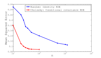
We now focus on the scalability of our method and consider the face-to-face mapping problem with a large number of examples. Here we use all the rotated face images (30, 60, and 90 degree left and right rotations) to predict the plain face expression. This gives us 1,200 examples for training and 200 for testing. Fig. 2 compares the performance of the efficient implementation (using incomplete Cholesky decomposition) of our conditional covariance operator-valued KDE method with the original KDE algorithm (Cortes et al., 2005). The parameter $n$ is the number of faces randomly selected from 1,200 training faces in the original KDE and is $m_{1}=m_{2}=n$ in the incomplete Cholesky decomposition. The results indicate that the low-rank approximation of our KDE method leads to both a considerable reduction in computation time and a good performance. It obtains a better MSE with $m_{1}=m_{2}=30$ than the original KDE with all 1,200 examples.

Figure 2: We compare the efficient implementation (using incomplete Cholesky decomposition) of our conditional covariance operator-valued KDE method with the KDE algorithm of Cortes et al. (2005). While the parameter $n$ is $m_{1}=m_{2}=n$ in the incomplete Cholesky decomposition, it is the number of faces randomly selected from 1,200 training faces in the KDE algorithm of Cortes et al. (2005). The right-most point is the MSE of training on the full training set of $n=1,200$ examples.

7 Conclusions and Future Work

In this paper, we presented a general formulation of kernel dependency estimation (KDE) for structured output learning using operator-valued kernels, and illustrated its use in several experiments. We also proposed a new covariance-based operator-valued kernel that takes into account the structure of the output kernel feature space. This kernel encodes the interactions between the outputs, but makes no reference to the input space. We addressed this issue by introducing a variant of our KDE method based on the conditional covariance operator that in addition to the correlation between the outputs takes into account the effects of the input variables.

In our work, we focused on regression-based structured output prediction. An interesting direction for future research is to explore operator-valued kernels in the context of classification-based structured output learning. Joint kernels and operator-valued kernels have strong connections, but more investigation is needed to show how operator-valued kernel formulation can be used to improve joint kernel methods, and how to deal with the pre-image problem in this case.

8 Appendix

8.1 (Generalized) Kernel Trick

In this section, we prove the (generalized) kernel trick used in Section 3 of the paper, i.e., $\langle\mathcal{T}\Phi_{l}(y_{1}),\Phi_{l}(y_{2})\rangle_{\mathcal{F_{Y}}}=[\mathcal{T}l(y_{1},\cdot)](y_{2})$, where $\mathcal{T}\in\mathcal{L(F_{Y})}$ and $\mathcal{F_{Y}}$ is a RKHS with kernel $l$.

Case 1: $\Phi_{l}$ is the feature map associated to the reproducing kernel $l$, i.e., $\Phi_{l}(y)=l(\cdot,y)$.

Here the proof is straightforward, we may write

$$\langle\mathcal{T}\Phi_{l}(y_{1}),\Phi_{l}(y_{2})\rangle_{\mathcal{F_{Y}}}=\langle\mathcal{T}l(\cdot,y_{1}),l(\cdot,y_{2})\rangle_{\mathcal{F_{Y}}}=[\mathcal{T}l(y_{1},\cdot)](y_{2}).$$

The second equality follows from the reproducing property.

Case 2: $\Phi_{l}$ is an implicit feature map of a Mercer kernel, and $\mathcal{T}$ is a self-adjoint operator in $\mathcal{L(F_{Y})}$.

We first recall the Mercer’s theorem:

Theorem 2 (Mercer’s theorem)

Suppose that $l$ is a symmetric real-valued kernel on $\mathcal{Y}^{2}$ such that the integral operator $T_{l}:L_{2}(\mathcal{Y})\rightarrow L_{2}(\mathcal{Y})$, defined as

$$(T_{l}f)(y_{1}):=\int_{\mathcal{Y}}l(y_{1},y_{2})f(y_{2})dy_{2}$$

is positive. Let $\gamma_{j}\in L_{2}(\mathcal{Y})$ be the normalized eigenfunctions of $T_{l}$ associated with the eigenvalues $\lambda_{j}>0$, sorted in non-increasing order. Then

$$l(y_{1},y_{2})=\sum_{j=1}^{N_{f}}\lambda_{j}\gamma_{j}(y_{1})\gamma_{j}(y_{2})$$ (9)

holds for almost all $(y_{1},y_{2})$ with $N_{f}\in\mathbb{N}$.

Since $l$ is a Mercer kernel, the eigenfunctions $(\gamma_{i})_{i=1}^{N_{f}}$ can be chosen to be orthogonal w.r.t. the dot product in $L_{2}(\mathcal{Y})$. Hence, it is straightforward to construct a dot product $\langle\cdot,\cdot\rangle$ such that $\langle\gamma_{i},\gamma_{j}\rangle=\delta_{ij}/\lambda_{j}$ ($\delta_{ij}$ is the Kronecker delta) and the orthonormal basis $\big{(}e_{j}\big{)}_{j=1}^{N_{f}}=\big{(}\sqrt{\lambda_{j}}\gamma_{j}\big{)}_{j=1}^{N_{f}}$ (see (Schölkopf et al., 1999) for more details). Therefore, the feature map associated to the Mercer kernel $l$ is of the form

$$\Phi_{l}:y\longmapsto\big{(}\sqrt{\lambda_{j}}\gamma_{j}(y)\big{)}_{j=1}^{N_{f}}\;.$$

Using (9), we can compute $[\mathcal{T}l(y_{1},\cdot)](y_{2})$ as follows:

$$[\mathcal{T}l(y_{1},\cdot)](y_{2}) =\sum_{j=1}^{N_{f}}\lambda_{j}\gamma_{j}(y_{1})\big{[}\mathcal{T}\gamma_{j}\big{]}(y_{2})$$

$$=\sum_{i,j=1}^{N_{f}}\lambda_{j}\gamma_{j}(y_{1})\langle\mathcal{T}\gamma_{j},e_{i}\rangle e_{i}(y_{2})$$

$$=\ \sum_{i,j=1}^{N_{f}}\lambda_{j}\gamma_{j}(y_{1})\lambda_{i}\langle\mathcal{T}\gamma_{j},\gamma_{i}\rangle\gamma_{i}(y_{2}).$$ (10)

Let $\widehat{\mathcal{T}}=\big{(}\widehat{\mathcal{T}}_{ij}\big{)}_{i,j=1}^{N_{f}}$ be the matrix representation of the operator $\mathcal{T}$ in the basis $\big{(}e_{j}\big{)}_{j=1}^{N_{f}}$. By definition we have $\widehat{\mathcal{T}}_{ij}=\langle\mathcal{T}e_{i},e_{j}\rangle$. Using this and the feature map expression of a Mercer kernel, we obtain

$$\langle\mathcal{T}\Phi_{l}(y_{1}) ,\Phi_{l}(y_{2})\rangle_{\mathcal{F_{Y}}}=\sum_{i=1}^{N_{f}}\big{(}\widehat{\mathcal{T}}\Phi_{l}(y_{1})\big{)}_{i}\big{(}\Phi_{l}(y_{2})\big{)}_{i}$$

$$=\sum_{i=1}^{N_{f}}\left(\sum_{j=1}^{N_{f}}\widehat{\mathcal{T}}_{ij}\sqrt{\lambda_{j}}\gamma_{j}(y_{1})\right)\sqrt{\lambda_{i}}\gamma_{i}(y_{2})$$

$$=\sum_{i,j=1}^{N_{f}}\langle\mathcal{T}e_{i},e_{j}\rangle\sqrt{\lambda_{j}}\gamma_{j}(y_{1})\sqrt{\lambda_{i}}\gamma_{i}(y_{2})$$

$$=\sum_{i,j=1}^{N_{f}}\langle\mathcal{T}\sqrt{\lambda_{i}}\gamma_{i},\sqrt{\lambda_{j}}\gamma_{j}\rangle\sqrt{\lambda_{j}}\gamma_{j}(y_{1})\sqrt{\lambda_{i}}\gamma_{i}(y_{2})$$

$$=\sum_{i,j=1}^{N_{f}}\lambda_{j}\gamma_{j}(y_{1})\langle\mathcal{T}\gamma_{i},\gamma_{j}\rangle\lambda_{i}\gamma_{i}(y_{2})$$

$$=\sum_{i,j=1}^{N_{f}}\lambda_{j}\gamma_{j}(y_{1})\langle\mathcal{T}\gamma_{j},\gamma_{i}\rangle\lambda_{i}\gamma_{i}(y_{2}).$$ (11)

Note that the last equality follows from the fact that $\mathcal{T}$ is a self-adjoint operator. The proof follows from Eqs. 8.1 and 8.1.

8.2 Proof of Proposition 1

In this section, we provide the proof of Proposition 1. We only show the proof for the covariance-based operator-valued kernels, since the proof for the other case (conditional covariance-based operator-valued kernels) is quite similar. Note that the pre-image problem is of the form

$$f(x)=\operatorname*{arg\,min}\limits_{y\in\mathcal{Y}}\;l(y,y)-2\big{[}\mathbf{K}_{x}(\mathbf{K}+\lambda I)^{-1}\mathbf{L}_{\bullet}\big{]}(y),$$

and our goal is to compute its Gram matrix expression in case $K(x_{i},x_{j})=k(x_{i},x_{j})\widehat{C}_{YY}^{(n)}$, where $\widehat{C}_{YY}^{(n)}$ is the empirical covariance operator defined as

$$\widehat{C}_{YY}^{(n)}=\frac{1}{n}\sum\limits_{i=1}^{n}l(\cdot,y_{i})\otimes l(\cdot,y_{i}).$$

Let $h=(h_{i})_{i=1}^{n}$ be a vector of variables in the RKHS $\mathcal{F_{Y}}$ such that $h=(\mathbf{K}+\lambda I)^{-1}\mathbf{L}_{\bullet}$. Since each $h_{i}$ is in the RKHS $\mathcal{F_{Y}}$, it can be decomposed as

$$h_{i}=\alpha_{(i)}^{\top}\mathbf{L}_{\bullet}+h_{i\bot}=\sum\limits_{j=1}^{n}\alpha_{(i)}^{j}l(\cdot,y_{j})+h_{i\bot},$$

where $\alpha_{(i)}\in\mathbb{R}^{n}$, $\mathbf{L}_{\bullet}=\big{(}l(\cdot,y_{1}),\ldots,l(\cdot,y_{n})\big{)}^{\top}$, and $h_{i\bot}$ is orthogonal to all $l(\cdot,y_{i})$’s, $i=1,\ldots,n$. The idea here is similar to the one used by Fukumizu et al. (2011). Now we may write

$$(\mathbf{K}+\lambda I)h=\mathbf{L}_{\bullet},$$

which gives us

$$\forall i\in{1,\ldots,n}\quad\quad l(\cdot,y_{i})=\sum_{j=1}^{n}\mathbf{K}_{ij}h_{j}+\lambda h_{i}.$$

Using the empirical covariance operator, for each $i$, we may write

$$l(\cdot,y_{i}) =\sum_{j=1}^{n}k(x_{i},x_{j})\widehat{C}_{YY}^{(n)}h_{j}+\lambda h_{i}$$

$$=\sum_{j=1}^{n}k(x_{i},x_{j})\Big{(}\frac{1}{n}\sum_{s=1}^{n}l(\cdot,y_{s})\otimes l(\cdot,y_{s})\Big{)}h_{j}+\lambda h_{i}$$

$$=\sum_{j=1}^{n}\frac{1}{n}k(x_{i},x_{j})\Big{(}\sum_{s=1}^{n}l(\cdot,y_{s})\otimes l(\cdot,y_{s})\Big{)}\Big{(}\sum_{m=1}^{n}\alpha_{(j)}^{m}l(\cdot,y_{m})+h_{i\bot}\Big{)}+\lambda\sum_{m=1}^{n}\alpha_{(i)}^{m}l(\cdot,y_{m})+\lambda h_{i\bot}$$

$$=\sum_{j=1}^{n}\frac{1}{n}k(x_{i},x_{j})\sum_{s=1}^{n}\sum_{m=1}^{n}\alpha_{(j)}^{m}l(y_{s},y_{m})l(\cdot,y_{s})+0+\lambda\mathbf{L}_{\bullet}^{\top}\alpha_{(i)}+\lambda h_{i\bot}$$

$$=\sum_{j=1}^{n}\frac{1}{n}k(x_{i},x_{j})\sum_{s=1}^{n}l(\cdot,y_{s})\sum_{m=1}^{n}\alpha_{(j)}^{m}l(y_{s},y_{m})+\lambda\mathbf{L}_{\bullet}^{\top}\alpha_{(i)}+\lambda h_{i\bot}$$

$$=\sum_{j=1}^{n}\frac{1}{n}k(x_{i},x_{j})\mathbf{L}_{\bullet}^{\top}\mathbf{L}\alpha_{(j)}+\lambda\mathbf{L}_{\bullet}^{\top}\alpha_{(i)}+\lambda h_{i\bot}.$$

Now if take the inner-product of the above equation with all $l(y_{s},\cdot),\;s=1,\ldots,n$, we obtain that for each $i$

$$l(y_{i},y_{s}) =\sum_{j=1}^{n}\frac{1}{n}k(x_{i},x_{j})\langle l(\cdot,y_{s}),\mathbf{L}_{\bullet}^{\top}\mathbf{L}\alpha_{(j)}\rangle+\lambda\langle l(\cdot,y_{s}),\mathbf{L}_{\bullet}^{\top}\alpha_{(i)}\rangle+\lambda\langle l(\cdot,y_{s}),h_{i\bot}\rangle$$

$$=\sum_{j=1}^{n}\frac{1}{n}k(x_{i},x_{j})\mathbf{L}_{y_{s}}^{\top}\mathbf{L}\alpha_{(j)}+\lambda\mathbf{L}_{y_{s}}^{\top}\alpha_{(i)},$$

which gives us the vector form

$$\mathbf{L}_{y_{i}}=\sum_{j=1}^{n}\frac{1}{n}k(x_{i},x_{j})\mathbf{L}\mathbf{L}\alpha_{(j)}+\lambda\mathbf{L}\alpha_{(i)}.$$ (12)

Defining the $n\times n$ matrix $\boldsymbol{\alpha}=(\alpha_{(1)},\ldots,\alpha_{(n)})$, we may write Eq. 12 in a matrix form as

$$\mathbf{L}=\frac{1}{n}\mathbf{L}\mathbf{L}\boldsymbol{\alpha}\mathbf{k}+\lambda\mathbf{L}\boldsymbol{\alpha},$$

which gives us

$$\frac{1}{n}\mathbf{L}\boldsymbol{\alpha}\mathbf{k}+\lambda\boldsymbol{\alpha}=I_{n}.$$

Using $\operatorname{vec}(ABC)=(C^{\top}\otimes A)\operatorname{vec}(B)$, we have

$$\big{(}\frac{1}{n}\mathbf{k}\otimes\mathbf{L}+\lambda I_{n^{2}}\big{)}\operatorname{vec}(\boldsymbol{\alpha})=\operatorname{vec}(I_{n}).$$ (13)

Now we may write

$$\mathbf{K}_{x}(\mathbf{K}+\lambda I)^{-1}\mathbf{L}_{\bullet}\ =\ \mathbf{K}_{x}h=\sum_{i=1}^{n}K(x,x_{i})h_{i}$$

$$=\sum_{i=1}^{n}k(x,x_{i})\widehat{C}_{YY}^{(n)}h_{i}=\sum_{i=1}^{n}\frac{1}{n}k(x,x_{i})\mathbf{L}_{\bullet}^{\top}\mathbf{L}\alpha_{(i)}$$

$$=\frac{1}{n}\mathbf{L}_{\bullet}^{\top}\mathbf{L}\boldsymbol{\alpha}\mathbf{k}_{x}=\frac{1}{n}\mathbf{L}_{\bullet}^{\top}\operatorname{vec}(\mathbf{L}\boldsymbol{\alpha}\mathbf{k}_{x})=\frac{1}{n}\mathbf{L}_{\bullet}^{\top}\big{(}\mathbf{k}^{\top}_{x}\otimes\mathbf{L}\big{)}\operatorname{vec}(\boldsymbol{\alpha})$$

$$=\mathbf{L}_{\bullet}^{\top}\big{(}\mathbf{k}^{\top}_{x}\otimes\mathbf{L}\big{)}\big{(}\mathbf{k}\otimes\mathbf{L}+n\lambda I_{n^{2}}\big{)}^{-1}\operatorname{vec}(I_{n}),$$

where the last equality comes from (13). Thus, we may write

$$f(x)\\ =\operatorname*{arg\,min}\limits_{y\in\mathcal{Y}}\;l(y,y)-2\mathbf{L}_{y}^{\top}(\mathbf{k}^{\top}_{x}\otimes\mathbf{L})(\mathbf{k}\otimes\mathbf{L}+n\lambda I_{n^{2}})^{-1}\operatorname{vec}(I_{n}),$$

which concludes the proof.

8.3 Computational Complexity of Solving the Pre-image Problem

As discussed in Section 4, solving the pre-image problem of Eq. 8 requires computing the following expression:

$$C(x,y)\\ =l(y,y)-2\mathbf{L}_{y}^{\top}(\mathbf{k}^{\top}_{x}\otimes\mathbf{L})(\mathbf{k}\otimes\mathbf{L}+n\lambda I_{n^{2}})^{-1}\operatorname{vec}(I_{n}).$$ (14)

Simple computation of $C(x,y)$ requires storing and inverting the matrix $(\mathbf{k}\otimes\mathbf{L}+n\lambda I_{n^{2}})\in\mathbb{R}^{n^{2}\times n^{2}}$. This leads to space and computational complexities of order $O(n^{4})$ and $O(n^{6})$. In this section, we provide an efficient procedure to for this computation that reduces its space and computational complexities to $O\big{(}\max(nm_{1}m_{2}\;,\;m_{1}^{2}m_{2}^{2})\big{)}$ and $O(m_{1}^{3}m_{2}^{3})$.

We first apply incomplete Cholesky decomposition to the kernel matrices $\mathbf{k}\in\mathbb{R}^{n\times n}$ and $\mathbf{L}\in\mathbb{R}^{n\times n}$ (Bach & Jordan, 2002). This consists of finding the matrices $\mathbf{U}\in\mathbb{R}^{n\times m_{1}}$ and $\mathbf{V}\in\mathbb{R}^{n\times m_{2}}$, with $m_{1}\ll n$ and $m_{2}\ll n$, such that

$$\mathbf{k}=\mathbf{U}\mathbf{U}^{\top}\quad\quad\quad,\quad\quad\quad\mathbf{L}=\mathbf{V}\mathbf{V}^{\top}.$$

Using this decomposition in (14), we obtain

$$C(x,y) =l(y,y)-2\mathbf{L}_{y}^{\top}(\mathbf{k}^{\top}_{x}\otimes\mathbf{L})[\mathbf{U}\mathbf{U}^{\top}\otimes\mathbf{V}\mathbf{V}^{\top}+n\lambda I_{n^{2}}]^{-1}\operatorname{vec}(I_{n})$$

$$\stackrel{{\scriptstyle(a)}}{{=}}l(y,y)-2\mathbf{L}_{y}^{\top}(\mathbf{k}^{\top}_{x}\otimes\mathbf{L})\big{[}(\mathbf{U}\otimes\mathbf{V})(\mathbf{U}^{\top}\otimes\mathbf{V}^{\top})+n\lambda I_{n^{2}}\big{]}^{-1}\operatorname{vec}(I_{n})$$

$$\stackrel{{\scriptstyle(b)}}{{=}}l(y,y)-\frac{2}{n\lambda}\mathbf{L}_{y}^{\top}(\mathbf{k}^{\top}_{x}\otimes\mathbf{L})\Big{[}I_{n^{2}}-(\mathbf{U}\otimes\mathbf{V})\big{(}n\lambda I_{m_{1}m_{2}}+(\mathbf{U}^{\top}\otimes\mathbf{V}^{\top})(\mathbf{U}\otimes\mathbf{V})\big{)}^{-1}(\mathbf{U}^{\top}\otimes\mathbf{V}^{\top})\Big{]}\operatorname{vec}(I_{n})$$

$$\stackrel{{\scriptstyle(c)}}{{=}}l(y,y)-\frac{2}{n\lambda}\mathbf{L}_{y}^{\top}(\mathbf{k}^{\top}_{x}\otimes\mathbf{L})\big{[}\operatorname{vec}(I_{n})-(\mathbf{U}\otimes\mathbf{V})(n\lambda I_{m_{1}m_{2}}+\mathbf{U}^{\top}\mathbf{U}\otimes\mathbf{V}^{\top}\mathbf{V})^{-1}(\mathbf{U}^{\top}\otimes\mathbf{V}^{\top})\operatorname{vec}(I_{n})\big{]}$$

$$=l(y,y)-\frac{2}{n\lambda}\mathbf{L}_{y}^{\top}\big{[}(\mathbf{k}^{\top}_{x}\otimes\mathbf{L})\operatorname{vec}(I_{n})-(\mathbf{k}^{\top}_{x}\otimes\mathbf{L})(\mathbf{U}\otimes\mathbf{V})(n\lambda I_{m_{1}m_{2}}+\mathbf{U}^{\top}\mathbf{U}\otimes\mathbf{V}^{\top}\mathbf{V})^{-1}(\mathbf{U}^{\top}\otimes\mathbf{V}^{\top})\operatorname{vec}(I_{n})\big{]}$$

$$\stackrel{{\scriptstyle(d)}}{{=}}l(y,y)-\frac{2}{n\lambda}\mathbf{L}_{y}^{\top}\big{[}\operatorname{vec}(\mathbf{L}\mathbf{k}_{x})-(\mathbf{k}^{\top}_{x}\mathbf{U}\otimes\mathbf{L}\mathbf{V})(n\lambda I_{m_{1}m_{2}}+\mathbf{U}^{\top}\mathbf{U}\otimes\mathbf{V}^{\top}\mathbf{V})^{-1}\operatorname{vec}(\mathbf{V}^{\top}\mathbf{U})\big{]}$$

$$\stackrel{{\scriptstyle(e)}}{{=}}l(y,y)-\frac{2}{n\lambda}\mathbf{L}_{y}^{\top}\big{[}\mathbf{L}\mathbf{k}_{x}-(\mathbf{k}^{\top}_{x}\mathbf{U}\otimes\mathbf{L}\mathbf{V})(n\lambda I_{m_{1}m_{2}}+\mathbf{U}^{\top}\mathbf{U}\otimes\mathbf{V}^{\top}\mathbf{V})^{-1}\operatorname{vec}(\mathbf{V}^{\top}\mathbf{U})\big{]}$$ (15)

(a) and (c) follow from the fact that $\;\;\;(\mathbf{A}\otimes\mathbf{B})(\mathbf{C}\otimes\mathbf{D})=\mathbf{AC}\otimes\mathbf{BD}$.

(b) follows from the Woodbury formula, i.e., $(\mathbf{A}+\mathbf{BC})^{-1}=\mathbf{A}^{-1}-\mathbf{A}^{-1}\mathbf{B}(\mathbf{I}+\mathbf{CA}^{-1}\mathbf{B})^{-1}\mathbf{CA}^{-1}$.

(d) follows from the fact that $\;\;\;\operatorname{vec}(\mathbf{ABC})=(\mathbf{C}^{\top}\otimes\mathbf{A})\operatorname{vec}(\mathbf{B})$.

(e) follows from the fact that $\mathbf{L}\mathbf{k}_{x}$ is a $n\times 1$ vector.

The most expensive computations in Eq. 8.3 is the inversion of matrix $(n\lambda I_{m_{1}m_{2}}+\mathbf{U}^{\top}\mathbf{U}\otimes\mathbf{V}^{\top}\mathbf{V})\in\mathbb{R}^{m_{1}m_{2}\times m_{1}m_{2}}$, with computational cost of order $O(m_{1}^{3}m_{2}^{3})$. Therefore, we have reduced the cost of computing $C(x,y)$ from $O(n^{6})$ to $O(m_{1}^{3}m_{2}^{3})$. Moreover, the largest size matrix that is needed to be stored in order to compute Eq. 8.3 is either $(n\lambda I_{m_{1}m_{2}}+\mathbf{U}^{\top}\mathbf{U}\otimes\mathbf{V}^{\top}\mathbf{V})\in\mathbb{R}^{m_{1}m_{2}\times m_{1}m_{2}}$ or $(\mathbf{k}^{\top}_{x}\mathbf{U}\otimes\mathbf{L}\mathbf{V})\in\mathbb{R}^{n\times m_{1}m_{2}}$, which reduces the space complexity from $O(n^{4})$ to $O\big{(}\max(nm_{1}m_{2}\;,\;m_{1}^{2}m_{2}^{2})\big{)}$.

References

- Álvarez et al. (2012) Álvarez, M., Rosasco, L., and Lawrence, N. D. Kernels for vector-valued functions: a review. Foundations and Trends in Machine Learning, 4(3):195–266, 2012.
- Bach & Jordan (2002) Bach, F. and Jordan, M. Kernel independent component analysis. Journal of Machine Learning Research, 3:1–48, 2002.
- Bakir et al. (2007) Bakir, G., Hofmann, T., Schölkopf, B., Smola, A., Taskar, B., and Vishwanathan, S. (eds.). Predicting Structured Data. MIT Press, 2007.
- Brouard et al. (2011) Brouard, C., d’Alché Buc, F., and Szafranski, M. Semi-supervised penalized output kernel regression for link prediction. In Proc. ICML, pp. 593–600, 2011.
- Caponnetto & De Vito (2007) Caponnetto, A. and De Vito, E. Optimal rates for the regularized least-squares algorithm. Foundations of Computational Mathematics, 7(3):331–368, 2007.
- Caponnetto et al. (2008) Caponnetto, A., Micchelli, C., Pontil, M., and Ying, Y. Universal multi-task kernels. Journal of Machine Learning Research, 68:1615–1646, 2008.
- Caruana (1997) Caruana, R. Multitask learning. Machine Learning, 28(1):41–75, 1997.
- Cortes et al. (2005) Cortes, C., Mohri, M., and Weston, J. A general regression technique for learning transductions. In Proc. ICML, pp. 153–160, 2005.
- Cortes et al. (2007) Cortes, C., Mohri, M., and Weston, J. A General Regression Framework for Learning String-to-String Mappings. MIT Press, 2007.
- Evgeniou et al. (2005) Evgeniou, T., Micchelli, C., and Pontil, M. Learning multiple tasks with kernel methods. Journal of Machine Learning Research, 6:615–637, 2005.
- Fukumizu et al. (2004) Fukumizu, K., Bach, F., and Jordan, M. Dimensionality reduction for supervised learning with reproducing kernel hilbert spaces. Journal of Machine Learning Research, 5:73–99, 2004.
- Fukumizu et al. (2011) Fukumizu, K., Song, L., and Gretton, A. Kernel bayes’ rule. In Neural Information Processing Systems (NIPS), 2011.
- Gretton et al. (2005) Gretton, A., Herbrich, R., Smola, A., Bousquet, O., and Schölkopf, B. Kernel methods for measuring independence. Journal of Machine Learning Research, 6:1–47, 2005.
- Grunewalder et al. (2012) Grunewalder, S., Lever, G., Gretton, A., Baldassarre, L., Patterson, S., and Pontil, M. Conditional mean embeddings as regressors. In Proc. ICML, 2012.
- Kadri et al. (2010) Kadri, H., Duflos, E., Preux, P., Canu, S., and Davy, M. Nonlinear functional regression: a functional RKHS approach. In Proc. AISTATS, pp. 111–125, 2010.
- Kadri et al. (2011) Kadri, H., Rabaoui, A., Preux, P., Duflos, E., and Rakotomamonjy, A. Functional regularized least squares classification with operator-valued kernels. In Proc. ICML, pp. 993–1000, 2011.
- Kadri et al. (2012) Kadri, H., Ghavamzadeh, M., and Preux, P. A generalized kernel approach to structured output learning. Technical Report 00695631, INRIA, 2012.
- Micchelli & Pontil (2005) Micchelli, C. and Pontil, M. On learning vector-valued functions. Neural Computation, 17:177–204, 2005.
- Ramsay & Silverman (2005) Ramsay, J. and Silverman, B. Functional Data Analysis, 2nd edition. Springer Verlag, New York, 2005.
- Schölkopf et al. (1999) Schölkopf, B., Mika, S., Burges, C. J. C., Knirsch, P., Müller, K.-R., Rätsch, G., and Smola, A. J. Input space vs. feature space in kernel-based methods. IEEE Trans. on Neural Networks, 10(5):1000–1017, 1999.
- Taskar et al. (2004) Taskar, B., Guestrin, C., and Koller, D. Max-margin markov networks. In Advances in Neural Information Processing Systems 16. 2004.
- Troje & Bulthoff (1996) Troje, N. and Bulthoff, H. Face recognition under varying poses: The role of texture and shape. Vision Research, 36:1761–1771, 1996.
- Tsochantaridis et al. (2005) Tsochantaridis, I., Joachims, T., Hofmann, T., and Altun, Y. Large margin methods for structured and interdependent output variables. Journal of machine Learning Research, 6:1453–1484, 2005.
- Wang & Shawe-Taylor (2010) Wang, Z. and Shawe-Taylor, J. A kernel regression framework for SMT. Machine Translation, 24(2):87–102, 2010.
- Weston et al. (2003) Weston, J., Chapelle, O., Elisseeff, A., Schölkopf, B., and Vapnik, V. Kernel dependency estimation. In Proceedings of the Advances in Neural Information Processing Systems 15, pp. 873–880, 2003.
- Weston et al. (2007) Weston, J., BakIr, G., Bousquet, O., Schölkopf, B., Mann, T., and Noble, W. Joint Kernel Maps. MIT Press, 2007.