Measures and LMI for space launcher robust control validation

Abstract

We describe a new temporal verification framework for safety and robustness analysis of nonlinear control laws, our target application being a space launcher vehicle. Robustness analysis, formulated as a nonconvex nonlinear optimization problem on admissible trajectories corresponding to piecewise polynomial dynamics, is relaxed into a convex linear programming problem on measures. This infinite-dimensional problem is then formulated as a generalized moment problem, which allows for a numerical solution via a hierarchy of linear matrix inequality relaxations solved by semidefinite programming. The approach is illustrated on space launcher vehicle benchmark problems, in the presence of closed-loop nonlinearities (saturations and dead-zones) and axis coupling.

Keywords: space launcher control; safety; verification; robustness analysis; measures; moments; polynomials; LMI; convex optimization

1 Introduction

This work is carried out within the scope of the project SAFE-V (Space Application Flight control Enhancement of Validation Framework). The objective of this project is to analyse, develop and demonstrate effective design, verification and validation strategies and metrics for advanced guidance navigation and control systems. These new strategies should be implemented in an incremental manner in the traditional validation framework in order to be applicable both for current launchers validation and for future launcher and re-entry vehicle validation.

Control design performance and compliance with system specifications should be demonstrated by a suitable combination of stability analysis and simulation. This validation is made on a wide domain of variation of influent parameters; it includes worst case validation and Monte Carlo simulation for statistic requirements, see e.g. Rongier and Droz (1999) for Ariane 5 validation.

Generally speaking, the Monte Carlo method is a numerical integration method using sampling, which can be used, for example, to determine the quantities of interest of a variable of interest for a random input variable such as mean or standard deviation or probability density function. One of the most commonly used methods inside ASTRIUM ST for the confidence interval on a quantile estimation is Wilks formula, see OPENTURNS (2008). This formula of the confidence interval depending on the probability level and the number of samples can be used, for Monte Carlo only, in two ways: to determine the probability and confidence level for the values of samples chosen by the user, or in reverse to determine the number of simulations to be carried out for the values probability and confidence level chosen by the user. Monte Carlo simulations are widely used in traditional validation process and they are very robust because they do not require smoothing assumptions on the model neither importance factor assumptions on the parameters. The random events are simulated as they would occur naturally. The generic Monte Carlo method is however very time consuming, because a great number of simulations to demonstrate extreme level of probability (in general much more than $1/p$ simulations to estimate the probability of an event of probability $p$). The number of simulations required may be critical for long duration mission simulation (like launcher flight). In the context of robust control, see Tempo et al. (2005) for related probabilistic approaches. Note that these approaches may miss worst case behavior, especially when the number of parameters is large.

In contrast, worst case validation techniques are aimed at identifying worst case instances and behavior. These techniques include Lyapunov and mu-analysis approaches. Among them, the most relevant for space vehicle applications are:

• results by the GARTEUR group, see Fielding et al. (2002), and the COFCLUO group, see COFCLUO (2007), for recent aeronautic applications and new developments;

• results by ASTRIUM ST in the frame of ESA ITT for Robust LPV for launcher application, see ASTRIUM ST (2009a, b); Ganet-Schoeller and Maurice (2011), and for robust stability analysis for ATV industrial validation, see Ganet-Schoeller et al. (2009);

• results by NGC on rendezvous validation process in the frame of the ESA VVAF project, see Di Sotto et al. (2010a, b); Kron et al. (2010); Paulino et al. (2010), and on re-entry validation, see Kron and de Lafontaine (2004).

Many other non industrial applications are available in the literature. Two of them could be considered as major for our applications: a PhD thesis on missile application by Adounkpé (2004) and the IQC toolbox developed by Scherer and Köse (2008) with Delft University that was applied for HL-20 re-entry vehicle analysis in Veenman et al. (2009), under ESA contract.

In this paper we propose an original approach to validation of control laws based on measures and convex optimization over linear matrix inequalities (LMIs). The approach can be seen as a blend between worst case validation techniques and statistical simulation techniques. On the one hand, we optimize over worst case admissible trajectories to validate a system property. On the other hand, we propagate along system trajectories statistical information (probability measures) instead of deterministic initial conditions. Moreover, our approach is primal in the sense that we optimize directly over systems trajectories, we do not seek a dual Lyapunov certificate.

First we rephrase our validation problem as a robustness analysis problem, and then as a nonconvex nonlinear optimization problems over admissible trajectories. This is the approach followed e.g. in Prajna and Rantzer (2007) where the authors verify or prove temporal properties such as safety (all trajectories starting from a set of initial conditions never reach a set of bad states), avoidance (at least one trajectory starting from a set of initial conditions will never reach a set of bad states), eventuality (all trajectories starting from a set of initial conditions will reach a set of good states in finite time) and reachability (at least one trajectory starting from a set of initial conditions will reach a set of good states in finite time).

Following Lasserre et al. (2008), we formulate our nonconvex nonlinear trajectory optimization problem as a linear programming (LP) problem on measures, with at most three unknowns: the initial measure (modeling initial conditions), the occupation measure (encoding system trajectories) and the terminal measure (modeling terminal conditions); in some cases a subset of these decision variables may be given. The final time can be given or free, finite or infinite. If all the data are polynomials (performance measure, dynamics, constraints), then we formulate the infinite-dimensional LP on measures as a generalized moment problem (GMP), and we approach it via an asymptotically converging hierarchy of finite-dimensional convex LMI relaxations. These LMI relaxations are then modeled with our specialized software GloptiPoly 3, solved with a general-purpose semidefinite programming (SDP) solver, and system properties are validated from the numerical solutions.

The models we can deal with should be piecewise polynomial (or rational) in time and space. We consider a compact region of the state-space over which the trajectories are optimized. The system dynamics are defined locally on explicitly given basic semialgebraic sets (intersections of polynomial sublevel sets) by polynomial vector fields. The objective function (stability or performance measure) consists of a polynomial terminal term and of the time integral of a polynomial integrand.

Our contribution is to use the approach described in Lasserre et al. (2008) jointly with the corresponding software tool GloptiPoly 3 by Henrion et al. (2009) to address temporal validation/verification of control systems properties, in the applied context of space launcher applications. The use of LMI and measures was already investigated in Prajna and Rantzer (2007) for building Lyapunov barrier certificates, and based on a dual to Lyapunov’s theorem described in Ranzter (2001). Our approach is similar, in the sense that optimization over systems trajectories is formulated as an LP in the infinite-dimensional space of measures. This LP problem is then approached as a generalized moment problem via a hierarchy of LMI relaxations.

Historically, the idea of reformulating nonconvex nonlinear ordinary differential equations (ODE) into convex LP, and especially linear partial differential equations (PDE) in the space of probability measures, is not new. It was Joseph Liouville in 1838 who first introduced the linear PDE involving the Jacobian of the transformation exerted by the solution of an ODE on its initial condition Liouville (1838), see Ehrendorfer (1994, 2002) for a survey on the Liouville PDE with applications in meteorology. The idea was then largely expanded in Henri Poincaré’s work on dynamical systems at the end of the 19th century, see in particular (Poincaré, 1899, Chapitre XII (Invariants intégraux)). This work was pursued in the 20th century in Kryloff and Bogoliouboff (1937), (Nemystkii and Stepanov, 1947, Chapter VI (Systems with an integral invariant)) and more recently in the context of optimal transport by e.g. Rachev and Rüschendorf (1998), Villani (2003) or Ambrosio et al. (2008). Poincaré himself in (Poincaré, 1908, Section IV) mentions the potential of formulating nonlinear ODEs as linear PDEs, and this programme has been carried out to some extent by Carleman (1932), see also Lasota and Mackey (1985), Kowalski and Steeb (1991), Hernández-Lerma and Lasserre (2003) and more recently Barkley et al. (2006), Vaidya and Mehta (2008), Gaitsgory and Quincampoix (2009). For recent studies of the Liouville equation in optimal control see e.g. Kwee and Schmidhuber (2002) and Brockett (2007), and for applications in uncertainty propagation and control law validation see e.g. Mellodge and Kachroo (2008) and Halder and Bhattacharya (2011).

2 Piecewise polynomial dynamic optimization

Consider the following dynamic optimization problem with piecewise polynomial differential constraints

$$\begin{array}[]{lll}J\>=&\inf_{x(t)}&h_{T}(T,x(T))+\int_{0}^{T}h(t,x(t))dt\\ &\mathrm{s.t.}&\dot{x}(t)=f_{k}(t,x(t)),\>\>x(t)\in{X}_{k},\>\>k=1,2,\ldots,N\\ &&x(0)\in{X}_{0},\>\>x(T)\in{X}_{T},\>\>t\in[0,T]\end{array}$$ (1)

with given polynomial dynamics $f_{k}\in\mathbb{R}[t,x]$ and costs $h,h_{T}\in\mathbb{R}[t,x]$, and state trajectory $x(t)$ constrained in closed basic semialgebraic sets

$${X}_{k}=\{x\in\mathbb{R}^{n}\>:\>g_{kj}(t,x)\geq 0,\>j=1,2,\ldots,N_{k}\}$$

for given polynomials $g_{kj}\in\mathbb{R}[t,x]$. We assume that the state-space partitioning sets, or cells ${X}_{k}$, are disjoint, i.e. all their respective intersections have zero Lebesgue measure in $\mathbb{R}^{n}$, and they all belong to a given compact semialgebraic set, e.g.

$${X}=\{x\in\mathbb{R}^{n}\>:\>\|x\|^{2}_{2}\leq M\}$$

for a sufficiently large constant $M>0$. Finally, initial and terminal states are constrained in semialgebraic ets

$${X}_{0}=\{x\in\mathbb{R}^{n}\>:\>g_{0j}(t,x)\geq 0,\>j=1,2,\ldots,N_{0}\}\subset{X}$$

and

$${X}_{T}=\{x\in\mathbb{R}^{n}\>:\>g_{Tj}(t,x)\geq 0,\>j=1,2,\ldots,N_{T}\}\subset{X}$$

for given polynomials $g_{0j},g_{Tj}\in\mathbb{R}[t,x]$.

It is assumed that optimization problem (1) arises from validation of a controlled (closed-loop) system behavior. In this problem, the infimum is sought over absolutely continuous state trajectories $x(t)$, but the same methodology can be extended to (possibly discontinuous) trajectories of bounded variation (e.g. in the presence of impulsive controls or state jumps), see Claeys et al. (2011).

The final time $T$ is either given, or free, in which case it becomes a decision variable, jointly with $x(t)$. Similarly, the initial and terminal constraint sets ${X}_{0}$ and ${X}_{T}$ are either given, or free, in which case they also become optimized decision variables.

3 Linear programming on measures

In this section, we formulate optimization problem (1), which is nonlinear and nonconvex in state trajectory $x$, into a convex optimization problem linear in $\mu$, the occupation measure of trajectory $x$. This reformulation is classical in the modern theory of calculus of variations and optimal control and it can be traced back to Young (1937), see also Ghouila-Houri (1967), Young (1969) and Gamkrelidze (1975), amongst many others.

3.1 Occupation measure

To understand the basic idea behind the transformation and the elementary concept of occupation measure, it is better to deal with the single nonlinear ODE

$$\dot{x}_{t}=f(x_{t})$$ (2)

where $x_{t}$ is a shortcut for $x(t)$, a time-dependent state vector of $\mathbb{R}^{n}$ and $f:\mathbb{R}^{n}\to\mathbb{R}^{n}$ is a uniformly Lipschitz map. It follows that the Cauchy problem for ODE (2) has a unique solution $x_{t}$ for any given initial condition $x_{0}\in\mathbb{R}^{n}$.

Now think of initial condition $x_{0}$ as a random variable of $\mathbb{R}^{n}$, or more abstractly as a nonnegative probability measure $\mu_{0}$ with support ${X}_{0}\subset\mathbb{R}^{n}$, that is a map from the sigma-algebra of subsets of ${X}_{0}$ to the interval $[0,1]\subset\mathbb{R}$ such that $\mu_{0}({X}_{0})=1$. For example, the expected value of $x_{0}$ is the vector $E[x_{0}]=\int_{{X}_{0}}x\mu_{0}(dx)$.

Now solve ODE (2) for a trajectory, or flow $x_{t}$, given this random initial condition. At each time $t$, state $x_{t}$ can also be interpreted as a random variable, i.e. a probability measure that we denote by $\mu_{t}(dx)$. We say that the measure is transported by the flow of the ODE. The one-dimensional family, or path of measures $\mu_{t}$ satisfies a PDE

$$\frac{\partial\mu_{t}}{\partial t}+\mathrm{div}(f\mu_{t})=0$$ (3)

which turns out to be linear in the space of probability measures. This PDE is usually called Liouville’s equation. As explained e.g. in (Villani, 2003, Theorem 5.34), nonlinear ODE (1) follows by applying Cauchy’s method of characteristics to linear transport PDE (3), see also (Evans, 2010, Section 3.2) for a tutorial exposition. In equation (3), div models the divergence operator, i.e.

$$\mathrm{div}(v)=\sum_{i=1}^{n}\frac{\partial v_{i}}{\partial x_{i}}$$

for every smooth function $v$. Its action on measures should be understood in the weak, or distributional sense, i.e.

$$\int v\>\mathrm{div}(\nu)=-\int Dv\cdot d\nu$$

where $v$ is a smooth test function, $\nu$ is a vector-valued measure and $D$ stands for the gradient operator. Given a subset ${\mathcal{T}}\times{\mathcal{X}}$ in the sigma-algebra of subsets of $[0,T]\times X$, we define the occupation measure

$$\mu({\mathcal{T}}\times{\mathcal{X}})=\int_{\mathcal{T}}\mu_{t}({\mathcal{X}})dt$$

which encodes the time-space trajectories $x_{t}$, in the sense that $\mu([0,T]\times{\mathcal{X}})$ is the total time spent by trajectory $x_{t}$ in a subset ${\mathcal{X}}\subset X$ of the state space. In its integral form, transport PDE (3) becomes

$$\mathrm{div}(f\mu)=\mu_{0}-\mu_{T}$$ (4)

where $\mu_{T}$ is the terminal probability measure with support ${X}_{T}\subset\mathbb{R}^{n}$. PDE (4) can equivalently be formulated as

$$\int_{X}Dv\cdot fd\mu=\int_{{X}_{T}}vd\mu_{T}-\int_{{X}_{0}}vd\mu_{0}$$ (5)

for all smooth functions $v$ compactly supported on ${X}$. Problem (5) is an infinite-dimensional linear system of equations linking occupation measure $\mu$, initial measure $\mu_{0}$ and terminal measure $\mu_{T}$, consistently with ODE (2).

3.2 Finite terminal time

If we apply these ideas to problem (1), encoding the state trajectory $x(t)$ in an occupation measure $\mu$ supported on $X$, we come up with an infinite-dimensional LP problem

$$\begin{array}[]{lll}J_{\infty}\>=&\inf_{\mu}&\int h_{T}(T,x)d\mu_{T}(x)+\sum_{k}\int h(t,x)d\mu_{k}(t,x)\\ &\mathrm{s.t.}&\sum_{k}\int\frac{\partial v(t,x)}{\partial t}\>d\mu_{k}(t,x)\>\>+\\ &&\sum_{k}\int Dv(t,x)\cdot f_{k}(t,x)\>d\mu_{k}(t,x)\>\>=\\ &&\int v(T,x)\>d\mu_{T}(x)-\int v(0,x)\>d\mu_{0}(x)\end{array}$$ (6)

for all smooth test functions $v$, where each occupation measure $\mu_{k}$ is supported on set ${X}_{k}$ and the global occupation measure is

$$\mu=\sum_{k}\mu_{k}$$

with normalization constraint

$$\mu([0,T]\times{X})=T$$ (7)

such that $T$ is a finite terminal time.

In problem (6), final time $T$, initial measure $\mu_{0}$ and terminal measure $\mu_{T}$ may be given, or unknown, depending on the original optimization problem.

3.3 Generalized moment problem

More concisely, LP problem (6) can be formulated as follows:

$$\begin{array}[]{ll}\inf_{\mu}&\sum_{k}\int_{{X}_{k}}c_{k}\>d\mu_{k}\\ \mathrm{s.t.}&\sum_{k}\int_{{X}_{k}}a_{ki}\>d\mu_{k}=b_{i},\quad\forall i\end{array}$$ (8)

where the unknowns are a finite set of nonnegative measures $\mu_{k}$, with respective compact semialgebraic supports

$${X}_{k}=\{x\>:\>g_{kj}(x)\geq 0,\>\>\forall j\}.$$ (9)

Note that here we have incorporated time variable $t$ into vector $x$, for notational conciseness. If all the data in problem (6) are polynomials, and if we generate test functions $v(x)$ using a polynomial basis (e.g. monomials, which are dense in the set of continuous functions with compact support), all the coefficients $a(x)$, $b(x)$, $c(x)$ are polynomials, and there is an infinite but countable number of linear constraints indexed by $i$.

We will then manipulate each measure $\mu_{k}$ via its moments

$$y_{k\alpha}=\int_{{X}_{k}}x^{\alpha}d\mu_{k}(x),\quad\forall\alpha$$ (10)

gathered into an infinite-dimensional sequence $y_{k}$ indexed by a vector of integers $\alpha$, where we use the multi-index notation $x^{\alpha}=x_{1}^{\alpha_{1}}x_{2}^{\alpha_{2}}\ldots$ LP measure problem (8) becomes an LP moment problem, or GMP, see Lasserre (2009):

$$\begin{array}[]{ll}\inf_{y}&\sum_{k}\sum_{\alpha}c_{k\alpha}y_{k\alpha}\\ \mathrm{s.t.}&\sum_{k}\sum_{\alpha}a_{ki\alpha}y_{k\alpha}=b_{i},\quad\forall i\end{array}$$

provided we can handle the representation condition (10) which links a measure with its moments. It turns out (Lasserre, 2009, Chapter 3) that if sets ${X}_{k}$ are compact semialgebraic as in (9), we can use results of functional analysis and real algebraic geometry to design a hierarchy of LMI relaxations which is asymptotically equivalent to the generalized moment problem. In each LMI relaxation

$$\begin{array}[]{lll}J_{d}\>=&\inf_{y}&c^{T}y\\ &\mathrm{s.t.}&Ay=b\\ &&M_{d}(y)\succeq 0\\ &&M_{d}(g_{kj},y)\succeq 0,\quad\forall j,k\end{array}$$ (11)

we truncate the moment sequence to a finite number of its moments. If the highest moment power is $2d$, we call LMI relaxation of order $d$ the resulting finite-dimensional truncation. Matrix $M_{d}(y)$ is symmetric and linear in $y$, it is called the moment matrix, and it must be positive semidefinite for (10) to hold. Symmetric matrices $M_{d}(g_{kj},y)$ are also linear in $y$ and they are called localizing matrices. They ensure that the moments correspond to measures with appropriate supports. For $d$ finite, problem (11) is a finite-dimensional convex LP problem in the cone of positive semidefinite matrices, or SDP problem, for which off-the-shelf solvers are available, in particular implementations of the primal-dual interior-point methods described in Nesterov and Nemirovskii (1994).

3.4 Convergence

The hierarchy of LMI relaxations (11) generates an asymptotically converging monotonically increasing sequence of lower bounds on LP (6), i.e. $J_{d}\leq J_{d+1}$ for all $d=1,2\ldots$ and $\lim_{d\to\infty}J_{d}=J_{\infty}$. Obviously, the relaxed LP cost in problem (6) is a lower bound on the original cost in problem (1), i.e. $J_{\infty}\leq J$. Under mild assumptions, we can show that actually $J_{\infty}=J$, but the theoretical background required to prove this lies beyond the scope of this application paper.

3.5 Long range behavior

In the case terminal time $T$ tends to infinity, normalization constraint (7) becomes irrelevant, and the overall mass of occupation measure $\mu$ tends to infinity. A more appropriate formulation consists then of normalizing measure $\mu$ to a probability measure

$$\pi=\frac{\mu}{T}=\sum_{k}\frac{\mu_{k}}{T}=\sum_{k}\pi_{k}$$

so that PDE (4) becomes

$$\mathrm{div}(f\pi)=\lim_{T\to\infty}\frac{\mu_{0}-\mu_{T}}{T}=0$$

and LP problem (6) becomes

$$\begin{array}[]{ll}\inf_{\pi}&\sum_{k}\int h(t,x)d\pi_{k}(x)\\ \mathrm{s.t.}&\sum_{k}\int\frac{\partial v(t,x)}{\partial t}\>d\pi_{k}(x)\>\>+\\ &\sum_{k}\int Dv(t,x)\cdot f_{k}(t,x)\>d\pi_{k}(t,x)\>\>=0\\ \end{array}$$

where test functions $v(t,x)$ satisfy appropriate integrability and/or periodicity properties. Measure $\pi$ is called an invariant probability measure and it encodes equilibrium points, periodic orbits, ergodic behavior, possibly chaotic attractors, see e.g. Lasota and Mackey (1985), Diaconis and Freedman (1999), Hernández-Lerma and Lasserre (2003) and Gaitsgory and Quincampoix (2009).

4 Application to orbital launcher control law validation

In this section we report the application of our method to simplified models of an attitude control system (ACS) for a launcher in exo-atmospheric phase. We consider first a one degree-of-freedom (1DOF) model, and then a 3DOF model. The full benchmark is described in (SAFEV, 2011, Section 9) but it is not publicly available, and our computer codes cannot be distributed either.

4.1 ACS 1DOF

First we consider the simplified 1DOF model of launcher ACS in orbital phase. The closed-loop system must follow a given piecewise linear angular velocity profile. The original benchmark includes a time-delay and a pulsation width modulator in the control loop, but in our incremental approach we just discard these elements in a first approximation. See below for a description of possible extensions of our approach to time-delay systems. As to the pulsation width modulator, it can be handled if appropriately modeled as a parametric uncertainty.

4.1.1 Model

The system is modeled as a double integrator

$$I\ddot{\theta}(t)=u(t)$$

where $I$ is a given constant inertia and $u(t)$ is the torque control. We denote

$$x(t)=\left[\begin{array}[]{c}\theta(t)\\ \dot{\theta}(t)\end{array}\right]$$

and we assume that both angle $x_{1}(t)$ and angular velocity $x_{2}(t)$ are measured, and that the torque control is given by

$$u(x(t))=\mathrm{sat}(K^{T}\mathrm{dz}(x_{r}(t)-x(t)))$$

where $x_{r}(t)$ is the reference signal, $K\in{\mathbb{R}}^{2}$ is a given state feedback, $\mathrm{sat}$ is a saturation function such that $\mathrm{sat}(y)=y$ if $|y|\leq L$ and $\mathrm{sat}(y)=L\>\mathrm{sign}(y)$ otherwise, $\mathrm{dz}$ is a dead-zone function such that $\mathrm{dz}(x)=0$ if $|x_{i}|\leq D_{i}$ for some $i=1,2$ and $\mathrm{dz}(x)=1$ otherwise. Thresholds $L>0$, $D_{1}>0$ and $D_{2}>0$ are given.

We would like to verify whether the system state $x(t)$ reaches a given subset $X_{T}=\{x\in{\mathbb{R}}^{2}\>:\>x^{T}x\leq\varepsilon\}$ of the deadzone region after a fixed time $T$, and for all possible initial conditions $x(0)$ chosen in a given subset $X_{0}$ of the state-space, and for zero reference signals. We formulate an optimization problem (1) with systems dynamics defined as locally affine functions in three cells $X_{k}$, $k=1,2,3$ corresponding respectively to the linear regime of the torque saturation

$$X_{1}=\{x\in{\mathbb{R}}^{2}\>:\>|K^{T}x|\leq L\},\quad f_{1}(x)=\left[\begin{array}[]{c}x_{1}\\ -K^{T}x\end{array}\right]$$

the upper saturation regime

$$X_{2}=\{x\in{\mathbb{R}}^{2}\>:\>K^{T}x\geq L\},\quad f_{2}(x)=\left[\begin{array}[]{c}x_{1}\\ -L\end{array}\right]$$

and the lower saturation regime

$$X_{3}=\{x\in{\mathbb{R}}^{2}\>:\>K^{T}x\leq-L\},\quad f_{3}(x)=\left[\begin{array}[]{c}x_{1}\\ L\end{array}\right].$$

The objective function has no integral term and a concave quadratic terminal term $h_{T}(x)=-x(T)^{T}x(T)$ which we would like to minimize, so as to find trajectories with terminal states of largest norm. If we can certify that for every initial state $x(0)$ chosen in $X_{0}$ the final state $x(T)$ belongs to set included in the deadzone region, we have validated our controlled system.

4.1.2 Validation script

The resulting GloptiPoly 3 script, implementing some elementary scaling strategies to improve numerical behavior of the SDP solver, is as follows:

I = 27500; % inertia
kp = 2475; kd = 19800; % controller gains
L = 380; % input saturation level
dz1 = 0.2*pi/180; dz2 = 0.05*pi/180; % deadzone levels
thetamax = 50; omegamax = 5; % bounds on initial conditions
epsilon = sqrt(1e-5); % bound on norm of terminal condition
T = 50; % final time

d = input(’order of relaxation =’); d = 2*d;

% measures
mpol(’x1’,2); m1 = meas(x1); % linear regime
mpol(’x2’,2); m2 = meas(x2); % upper sat
mpol(’x3’,2); m3 = meas(x3); % lower sat
mpol(’x0’,2); m0 = meas(x0); % initial
mpol(’xT’,2); mT = meas(xT); % terminal

% dynamics on normalized time range [0,1]
% saturation input y normalized in [-1,1]
K = -[kp kd]/L;
y1 = K*x1; f1 = T*[x1(2); L*y1/I]; % linear regime
y2 = K*x2; f2 = T*[x2(2); L/I]; % upper sat
y3 = K*x3; f3 = T*[x3(2); -L/I]; % lower set

% test functions for each measure = monomials
g1 = mmon(x1,d); g2 = mmon(x2,d); g3 = mmon(x3,d);
g0 = mmon(x0,d); gT = mmon(xT,d);

% unknown moments of initial measure
y0 = mom(g0);

% unknown moments of terminal measure
yT = mom(gT);

% input LMI moment problem
cost = mom(xT’*xT);
Ay = mom(diff(g1,x1)*f1)+...
     mom(diff(g2,x2)*f2)+...
     mom(diff(g3,x3)*f3); % dynamics
% trajectory constraints
X = [y1^2<=1; y2>=1; y3<=-1];
% initial constraints
X0 = [x0(1)^2<=thetamax^2, x0(2)^2<=omegamax^2];
% terminal constraints
XT = [xT’*xT<=epsilon^2];
% bounds on trajectory
B = [x1’*x1<=4; x2’*x2<=4; x3’*x3<=4];

% input LMI moment problem
P = msdp(max(cost), ...
         mass(m1)+mass(m2)+mass(m3)==1, ...
         mass(m0)==1, ...
         Ay==yT-y0, ...
         X, X0, XT, B);

% solve LMI moment problem
[status,obj] = msol(P)

4.1.3 Numerical results

With this Matlab code and the SDP solver SeDuMi 1.3 (see sedumi.ie.lehigh.edu) we obtain the following sequence of upper bounds (since we maximize) on the maximum squared Euclidean norm of the final state:

relaxation order $d$	1	2	3	4
upper bound $J_{d}$	$1.0\cdot 10^{-5}$	$1.0\cdot 10^{-5}$	$1.0\cdot 10^{-5}$	$1.0\cdot 10^{-5}$
CPU time (sec.)	0.2	0.5	0.7	0.9
number of moments	30	75	140	225

In the table we also indicate the CPU time (in seconds, on a standard desktop computer) and the total number of moments (size of vector $y$ in the LMI relaxation (11). We see that the bound obtained at the first relaxation ($d=1$) is not modified for higher relaxations. This clearly indicates that all initial conditions are captured in the deadzone region at time $T$, which is the box $[-2,2]\frac{10^{-1}\pi}{180}\times[-5,5]\frac{10^{-2}\pi}{180}\supset\{x\in{\mathbb{R}}^{2}\>:\>x^{T}x\leq 10^{-5}\}$.

If we want to use this approach to simulate a particular trajectory, in the code we must modify the definition of the initial measure. For example for initial conditions $x_{1}(0)=50$, $x_{2}(0)=-1$, we must insert the following sequence:

% given moments of initial measure = Dirac at x0
p = genpow(3,d); p = p(:,2:end); % powers
theta0 = 50; omega0 = -1; % in degrees
y0 = ones(size(p,1),1)*[theta0 omega0]*pi/180;
y0 = prod(y0.^p,2);

As previously, the sequence of bounds on the maximum squared Euclidean norm of the final state is constantly equal to $1.0\cdot 10^{-5}$, and in the following table we represent as functions of the relaxation order $d$ the masses of measures $\mu_{k}$, $k=1,2,3$ which are indicators of the time spent by the trajectory in the respective linear, upper saturation and lower saturation regimes:

relaxation order $d$	1	2	3	4	5	6	7
$\int d\mu_{1}$	37	89	92	92	93	93	93
$\int d\mu_{2}$	32	5.3	0.74	0.30	0.21	0.15	0.17
$\int d\mu_{3}$	32	5.1	7.1	6.9	6.8	6.9	7.0

This indicates that most of the time (approx. 93%) is spent in the linear regime, with approx. 7% of the time spent in the lower saturation regime, and a negligible amount of time is spent in the upper saturation regime. This is confirmed by simulation, see Figure 1.

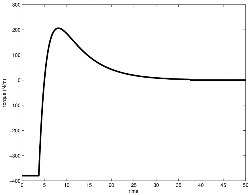
Figure 1: Torque input with lower saturation during approx. 7% of the time range.

4.2 Dealing with uncertainty

Finally, note that we can incorporate real parametric uncertainty in the dynamics, if required. Each uncertain parameter must be introduced as an additional state of the system, and this generally makes the dynamics polynomial in the extended state. The parameters must be constrained to an explicitly given compact semialgebraic set, and the overall trajectory optimization problem consists of finding the worst-case uncertain parameter instance.

For illustration, we modify the previous script to cope with uncertainty entering affinely the dynamics. We assume that the (reciprocal of the) inertia is subject to multiplicative relative uncertainty, i.e. we replace occurences of $I$ with $\frac{1}{1+u}I$ for $u$ a real parameter such that $u^{2}\leq U$ with $U>0$ a given threshold, say $U=\frac{1}{2}$. The resulting GloptiPoly 3 script is as follows:

I = 27500; % inertia
kp = 2475; kd = 19800; % controller gains
L = 380; % input saturation level
dz1 = 0.2*pi/180; dz2 = 0.05*pi/180; % deadzone levels
thetamax = 50; omegamax = 5; % bounds on initial conditions
epsilon = sqrt(1e-5); % bound on norm of terminal condition
T = 50; % final time

ui = 0.5; % uncertainty level (in percent)

d = input(’order of relaxation =’); d = 2*d;

% measures = states + uncertain parameter
mpol(’x1’,2); mpol u1; m1 = meas(x1,u1); % linear regime
mpol(’x2’,2); mpol u2; m2 = meas(x2,u2); % upper sat
mpol(’x3’,2); mpol u3; m3 = meas(x3,u3); % lower sat
mpol(’x0’,2); mpol u0; m0 = meas(x0,u0); % initial
mpol(’xT’,2); mpol uT; mT = meas(xT,uT); % terminal

% dynamics on normalized time range [0,1]
% saturation input y normalized in [-1,1]
K = -[kp kd]/L;
y1 = K*x1; f1 = T*[x1(2); (1+u1)*L*y1/I]; % linear regime
y2 = K*x2; f2 = T*[x2(2); (1+u2)*L/I]; % upper sat
y3 = K*x3; f3 = T*[x3(2); -(1+u3)*L/I]; % lower set

% test functions for each measure = monomials
g1 = mmon([x1;u1],d); g2 = mmon([x2;u2],d); g3 = mmon([x3;u3],d);
g0 = mmon([x0;u0],d); gT = mmon([xT;uT],d);

% unknown moments of initial measure
y0 = mom(g0);

% unknown moments of terminal measure
yT = mom(gT);

% input LMI moment problem
cost = mom(xT’*xT);
Ay = mom(diff(g1,x1)*f1)+...
     mom(diff(g2,x2)*f2)+...
     mom(diff(g3,x3)*f3); % dynamics
% trajectory constraints
X = [y1^2<=1; y2>=1; y3<=-1];
% initial constraints
X0 = [x0(1)^2<=thetamax^2, x0(2)^2<=omegamax^2];
% terminal constraints
XT = [xT’*xT<=epsilon^2];
% bounds on trajectory
B = [x1’*x1<=4; x2’*x2<=4; x3’*x3<=4];
% bounds on uncertain parameter
U = [u1^2<=ui^2; u2^2<=ui^2; u3^2<=ui^2];
U0 = [u0^2<=ui^2]; UT = [uT^2<=ui^2];

% input LMI moment problem
P = msdp(max(cost), ...
         mass(m1)+mass(m2)+mass(m3)==1, ...
         mass(m0)==1, ...
         Ay==yT-y0, ...
         X, X0, XT, B, ...
         U, U0, UT);

% solve LMI moment problem
[status,obj] = msol(P)

Introducing an uncertain parameter amounts to adding a state variable to the model, and this has a significant impact on the overall computational time, as shown in the table below:

relaxation order $d$	1	2	3	4
upper bound $J_{d}$	$1.0\cdot 10^{-5}$	$1.0\cdot 10^{-5}$	$1.0\cdot 10^{-5}$	$1.0\cdot 10^{-5}$
CPU time (sec.)	0.8	2.4	7.3	17.7
number of moments	75	224	501	946

Note however that for this example there is no effect on the bounds, and the control law is also validated in the presence of uncertainty on inertia.

4.3 ACS 3DOF

The main difficulty with the 3 degree-of-freedom version of the ACS benchmark is the large number of states (4 quaternions for the launcher attitude, 3 angular velocities, and 2 additional states for the quaternion reference signal) and the non-linear (quadratic) dynamics.

4.3.1 Model

The following example illustrates the validation of a given control law following a given constant roll velocity equal to $w^{R}_{1}=20^{o}/s$, in the absence of actuator saturation, but in the presence of non-linear coupling between the three axes of the launcher. System dynamics are given by $\dot{x}=f(x)$ with

$$x=\left[\begin{array}[]{c}q\\ w\\ q^{R}\end{array}\right],\quad f(x)=\left[\begin{array}[]{c}f_{q}(x)\\ f_{w}(x)\\ f_{q^{R}}(x)\end{array}\right],$$

and

$$f_{q}(x)=\frac{1}{2}Q(x)\left[\begin{array}[]{c}0\\ w\end{array}\right],$$

$$f_{w}(x)=I^{-1}(u(x)-\Omega(x)Iw),$$

$$f_{q^{R}}(x)=\left[\begin{array}[]{r}-\frac{1}{2}q^{R}_{1}w^{R}_{1}\\ \frac{1}{2}q^{R}_{0}w^{R}_{1}\end{array}\right]$$

where

$$Q(x)=\left[\begin{array}[]{rrrr}q_{0}&-q_{1}&-q_{2}&-q_{3}\\ q_{1}&q_{0}&-q_{3}&q_{2}\\ q_{2}&q_{3}&q_{0}&-q_{1}\\ q_{3}&-q_{2}&q_{1}&q_{0}\end{array}\right],\quad\Omega(x)=\left[\begin{array}[]{rrr}0&-w_{3}&w_{2}\\ w_{3}&0&-w_{1}\\ -w_{2}&w_{1}&0\end{array}\right],$$

$$u(x)=-K^{D}w^{E}-K^{P}q^{E},$$

$$K^{D}=\left[\begin{array}[]{ccc}K^{D}_{1}&0&0\\ 0&K^{D}_{2}&0\\ 0&0&K^{D}_{3}\\ \end{array}\right],\quad K^{P}=\left[\begin{array}[]{ccc}0&0&0\\ 0&K^{P}_{2}&0\\ 0&0&K^{P}_{3}\\ \end{array}\right],$$

$$w^{E}=\left[\begin{array}[]{c}w_{1}-w^{R}_{1}\\ w_{2}\\ w_{3}\end{array}\right],\quad q^{E}=2\left[\begin{array}[]{cccc}q^{R}_{0}&q^{R}_{1}&0&0\\ -q^{R}_{1}&q^{R}_{0}&0&0\\ 0&0&q^{R}_{0}&q^{R}_{1}\\ 0&0&-q^{R}_{1}&q^{R}_{0}\end{array}\right]q,$$

and $q\in{\mathbb{R}}^{4}$ is the quaternion modeling the attitude, $w\in{\mathbb{R}}^{3}$ models the angular velocities, $q^{R}\in{\mathbb{R}}^{2}$ is the reference quaternion to follow, which depends on the constant reference velocity $w^{R}_{1}\in{\mathbb{R}}$, $q^{E}\in{\mathbb{R}}^{4}$ is the quaternion error, and $w^{E}\in{\mathbb{R}}^{3}$ is the angular velocity error. Both vectors $q(t)$ and $q^{R}(t)$ have constant Euclidean norm since $\frac{d}{dt}\|q\|^{2}_{2}=2q^{T}\dot{q}=q^{T}f_{q}(x)=0$ for all $x$ and similarly $\frac{d}{dt}\|q^{R}\|^{2}_{2}=0$, so we enforce the algebraic constraints

$$\|q\|^{2}_{2}=1,\quad\|q^{R}\|^{2}_{2}=1.$$

The proportional-derivative control law $u(x)$ is designed so that velocity $w_{1}(t)$ follows reference velocity $w^{R}_{1}$, and our validation tasks consists of optimizing over the worst-case trajectory starting at a given initial condition $x(0)$ and maximizing the objective function

$$J=\int_{0}^{T}(w_{1}(t)-w^{R}_{1})^{2}dt$$

for a given time horizon $T$. If we can guarantee a sufficiently small upper bound $J_{d}$ on this objective function, for a given relaxation order $d=1,2,\ldots$, the control law is validated.

4.3.2 Validation script

We use the following GloptiPoly 3 script (note however that the function G2I to generate the inertia data is not available for the reader):

% Inertia
Ig = [ 27500,   -50, -1100;
         -50, 45300,  -220;
       -1100,  -220, 44100];
[Ge2In,Ip] = G2I(Ig);

% controller gains
w0 = 0.3; xi = 0.7;
Kp1 = Ip(1,1)*w0^2; Kd1 = 2*Ip(1,1)*xi*w0;
w0 = 0.25; xi = 3;
Kp2 = Ip(2,2)*w0^2; Kd2 = 2*Ip(2,2)*xi*w0;
Kp3 = Ip(3,3)*w0^2; Kd3 = 2*Ip(3,3)*xi*w0;

% initial conditions
Q0 = [1;0;0;0]; % attitude quaternion
W0 = [0;0;0].*(pi/180); % angular velocities

T = 50; % final time

% reference velocity
WR1 = 20*pi/180;

d = input(’order of relaxation =’);

% occupation measure
mpol(’q’,4); mpol(’w’,3); mpol(’qr’,2);
x = [q;w;qr]; m = meas(x);

% initial measure
mpol(’q0’,4); mpol(’w0’,3); mpol(’qr0’,2);
x0 = [q0;w0;qr0]; m0 = meas(x0);

% terminal measure
mpol(’qt’,4); mpol(’wt’,3); mpol(’qrt’,2);
xt = [qt;wt;qrt]; mt = meas(xt);

% dynamics on normalized time range [0,1]
Omega = [0 -w(3) w(2); w(3) 0 -w(1); -w(2) w(1) 0];
Qr = [qr(1) qr(2) 0 0;
      -qr(2) qr(1) 0 0;
      0 0 qr(1) qr(2);
      0 0 -qr(2) qr(1)];
dq = 2*Qr*q;
Q = [q(1) -q(2) -q(3) -q(4);
     q(2) q(1) -q(4) q(3);
     q(3) q(4) q(1) -q(2);
     q(4) -q(3) q(2) q(1)];
fq = 1/2*Q*[0;w];
Torque = [-Kd1*(w(1)-WR1);
          -Kd2*(w(2)-0)-Kp2*2*dq(3);
          -Kd3*(w(3)-0)-Kp3*2*dq(4)];
fw = Ig\(Torque-Omega*Ig*w);
fqr = [-1/2*qr(2)*WR1;1/2*qr(1)*WR1];
f = T*[fq;fw;fqr];

% test functions
g = mmon(x,d);
g0 = mmon(x0,d);
gt = mmon(xt,d);

% given moments of initial measure (Dirac)
p = genpow(10,d); p = p(:,2:end); % powers
y0 = ones(size(p,1),1)*[Q0’ W0’ 1 0];
y0 = prod(y0.^p,2);

% unknown moments of final measure
p = genpow(10,d); p = p(:,2:end); % powers
yt = ones(size(p,1),1)*[qt’ wt’ qrt’];
yt = mom(prod((yt.^p)’)’);

% input LMI moment problem
cost = mom((w(1)-WR1)^2); % objective function
Ay = mom(diff(g,x)*f); % dynamics
X = [q’*q == 1; qr’*qr == 1]; % quaternion
Xt = [qt’*qt == 1; qrt’*qrt == 1]; % final quaternion
P = msdp(max(cost), mass(m)==1, yt==Ay+y0, X, Xt);

% solve LMI moment problem
[status,obj] = msol(P)

4.3.3 Numerical results

We obtain the monotonically decreasing upper bounds $J_{d}$, $d=1,\ldots,4$ reported in the following table:

relaxation order $d$	1	2	3	4
upper bound $J_{d}$	$\infty$	$7.5198\cdot 10^{-3}$	$2.9110\cdot 10^{-3}$	$2.9085\cdot 10^{-3}$
CPU time (sec.)	0.2	11.6	24.2	2640
number of moments	110	770	1430	5720

The first LMI relaxation (110 moments of degree up to 2) seems to be unbounded above (the dual LMI problem is infeasible) and hence it conveys no useful information. The second LMI relaxation (770 moments of degree up to 3) and the third LMI relaxation (1430 moments of degree up to 4) are solved with SeDuMi 1.3 in a few seconds. The fourth LMI relaxation is more challenging, with 5720 moments of degree up to 5, and it requires less than one hour of CPU time on a standard PC. We observe however that a useful upper bound on $J$ is already obtained at a low relaxation order (say $d=2$ or $d=3$) at a low computational cost, and that the computational burden increases significantly for $d=4$ without dramatic improvements in the quality of the upper bound.

4.3.4 Coping with saturations and dead-zones

We can modify the above code to cope with actuator saturation and dead-zone, proceeding exactly as described above for the ACS 1DOF benchmark problem, namely by splitting the trajectory occupation measures into local occupation measures defined on semialgebraic (here polyhedral) cells. In the presence of saturations on the three actuators, this generates $3^{3}=27$ local occupation measures. This should not be an issue from the computational point of view, the limiting factor being essentially the size of the largest SDP block, which grows polynomially with the relaxation order, but with an exponent which is the number of variables (here equal to 10).

4.3.5 Following a time-varying reference signal

Finally, if we want to validate a control law to follow a time-varying velocity profile (instead of a constant velocity as above), we must introduce time as an additional variable in the trajectory occupation measure, we must introduce the velocity as an additional state, and we must split the occupation measure into local occupation measures, each of which corresponding to given time-invariant dynamics. Alternatively, we can also model time-varying dynamics, but the dependence on time must be polynomial (which is not the case e.g. if the reference signal is piecewise linear).

5 Discussion

In this section we discuss the limitations of our approach and we also describe possible extensions.

5.1 Limitations

The main limiting factor for our method is the total number of variables (number of states plus number of uncertain parameters), since the computational burden of solving the LMI relaxations grows polynomially as a function of the LMI relaxation order, but the order of the polynomial dependence depends linearly on the number of variables in the measures (here the number of states). So the critical dimension is not too much the number of measures (that is the number of cells partioning the state-space, which corresponds to our models of nonlinearities), or the degree of the polynomials in the cost and/or dynamics, but rather the number of states. Systems with a high number of states can be handled with these techniques, but only when exploiting problem structure and sparsity.

More explicitly, a rough complexity analysis can be carried out as follows. If an LMI relaxation has the simplified form

$$\begin{array}[]{ll}\inf_{y}&c^{T}y\\ \mathrm{s.t.}&M_{d}(y)\succeq 0\end{array}$$

where $M_{d}(y)$ is the moment matrix of a measure of $n$ variables at relaxation order $d$, then the number of variables in vector $y$ is

$$N=\left(\begin{array}[]{c}n+2d\\ n\end{array}\right)=\frac{(n+2d)!}{n!\,(2d)!}$$

and the size of matrix $M_{d}(y)$ is

$$M=\left(\begin{array}[]{c}n+d\\ n\end{array}\right)=\frac{(n+d)!}{n!\,d!}.$$

A standard primal-dual interior-point algorithm to solve this LMI at given relative accuracy $\epsilon>0$ (duality gap threshold) requires a number of iterations (Newton steps) growing as $O(M^{\frac{1}{2}}\log\epsilon)$, whose dependence on $M$ is sublinear, hence almost negligible. In practice, on well-conditioned problems, we observe that the number of Newton iterations is between 5 and 50, see Nesterov and Nemirovskii (1994), Vandenberghe and Boyd (1996) and Ben-Tal and Nemirovski (2001).

In the real model of computation (for which each addition, subtraction, multiplication, division of real numbers has unit cost), each Newton iteration requires $O(N^{2}M)+O(N^{3}M)+O(N^{2}M^{2})$ operations to form the linear system of equations, and $O(M^{3})$ operations to solve the system and find the search direction. When solving a hierarchy of simple LMI relaxations as described above, the number of variables $n$ is fixed, and the relaxation order $d$ varies, so the dominating term in the complexity estimate grows in $O(d^{4n})$, which clearly shows a strong dependence on the number of variables. Even though the growth of the computational burden is polynomial in the relaxation order, the exponent is 4 times the number of variables. One should however keep in mind that these estimates are (usually very loose) asymptotic upper bounds, and that the observed computational complexity grows much more moderately in practice (at least in the absence of conditioning and numerical stability issues).

Finally, if the LMI relaxation has the form

$$\begin{array}[]{ll}\inf_{y}&c^{T}y\\ \mathrm{s.t.}&M_{d}(y_{k})\succeq 0,\quad k=1,2,\ldots,K\end{array}$$

where $M_{d}(y_{k})$ is the moment matrix of a measure $\mu_{k}$ of $n$ variables at relaxation $d$, and we have $K$ measures, then the above complexity estimate grows in $O(Kd^{4n})$. The impact on the computation burden of the number $n$ of variables in each measure $\mu_{k}$ is thus much more critical than the number $K$ of measures. In our target application, $n$ is the number of states and uncertain parameters, $K$ is the number of cells used to model nonlinearities, and a lower bound on the minimum relaxation order $d$ is given by the degree of the polynomial data (dynamics, constraints, objective function).

5.1.1 Accuracy

The original validation problem can be formulated as infinite-dimensional linear programming problems on the dual cones of nonnegative measures and continuous functions, so that there is no hope of finite convergence of finite-dimensional LMI optimization techniques. Convergence is guaranteed only asymptotically. Obviously, the accuracy depends on the speed of convergence of the hierarchy of LMI problems, but this speed is impossible to evaluate a priori. The only guarantee is that we have a monotically increasing sequence of lower bounds on the objective function to be minimized.

As far as solving finite-dimensional LMI problems is concerned, we should emphasize the fact that there is currently no proof of backward stability of implementations of LMI solvers. Moreover, evaluation of the conditioning of a given LMI problem is difficult, and estimates can be obtained only at the price of solving several instances of (slightly modified versions) the original LMI problem. To certify the output of a numerical algorithm, we must simultaneously ensure backward stability of the algorithm and well-conditioning of the problem. None of these two properties can be ensured when solving LMI problems, given the current state-of-the-art in LMI solvers. But this is not specific to our method, and any validation-verification technique which is based on LMI optimization is subject to the same limitations.

5.1.2 Time-delay systems

Our techniques can in principle cope with time-delays, but this requires a significant modification of the approach described in this document. Let us only sketch the main ideas, in the case of an ordinary differential equation with one time-delay

$$\dot{x}(t)=f(x(t))+g(x(t-\tau)),\quad\forall t\in[0,T]$$

with boundary conditions

$$\quad x(t)=\xi(t),\>\>\forall t\in[-\tau,0]$$

where $\xi(t)$ is a given function recording the state history due to the given delay $\tau\in\mathbb{R}$. Instead of transporting a probability measure $\mu_{t}(dx)$ supported on $X\subset{\mathbb{R}}^{n}$ from initial time $t=0$ to terminal time $t=T$, we must transport the state history in an occupation measure $\mu_{t}(ds,dx)$ supported on $[-\tau,0]\times X$ for $t\in[0,T]$.

5.1.3 Discrete-time systems

In this paper we deal only with continuous-time systems. Discrete-time systems of the form

$$x_{k+1}=f(x_{k})$$ (12)

must be handled differently. Denoting by $\mu_{k}(x)$ the probability measure transported along dynamical system (12), the discrete-time analogue of Liouville’s transport equation (3) reads

$$\mu_{k+1}({\mathcal{X}})=\int_{f^{-1}({\mathcal{X}})}\mu_{k}(dx)=\int I_{\mathcal{X}}(f(x))\mu_{k}(dx)$$ (13)

where $\mathcal{X}$ is any subset of the sigma-algebra of state set $X$, and $I_{\mathcal{X}}$ is the indicator function equal to one in $\mathcal{X}$ and zero outside. It follows from (13) that the moments of measure $\mu_{k+1}$ can be expressed linearly as functions of moments of measure $\mu_{k}$. Besides this analogy, the resulting discrete-time generalized moment problem differs significantly from its continuous-time counterpart. For this reason, handling discrete-time systems would require an important modification of the approach described in this document.

6 Conclusion

In this paper we do not follow the mainstream Lyapunov approach to dynamical systems stability and/or performance validation. Lyapunov (1892) originally introduced his approach to conclude about systems behaviour while avoiding explicit computations of system trajectories. In the 1990s it was combined with LMI techniques, see e.g. Boyd et al. (1994); Nesterov and Nemirovskii (1994) to provide numerically quadratic certificates of stability and/or performance for linear and nonlinear systems. Later on, it was extended to more general, but still numerical polynomial sum-of-squares (SOS) certificates, see e.g. Henrion and Garulli (2005). By contrast, our approach is genuinely primal, in the sense that we directly optimize numerically over systems trajectories, using measures, moments and LMI techniques. Indeed, since the computation of SOS certificates is numerical anyway, we believe that in the context of validation, LMI techniques should rather be used to optimize systems trajectories, instead of optimizing indirect certificates for these trajectories. Since we are using primal-dual SDP solvers to solve the hierarchy of LMI problems, solving the dual to the problem of optimizing trajectories provides anyway certificates of feasibility or infeasibility, i.e. of stability, instability and/or performance.

As briefly described in §5, the measure/LMI approach can be extended easily to systems with real uncertainties, as soon as the uncertainties enter polynomially in the dynamics, and they are bounded in explicitly given semialgebraic sets (e.g. balls or boxes). See e.g. (Lasserre, 2009, Section 13.1) for more information on robust optimization. As usual, the number of real uncertain parameters should be kept small enough to ensure computational tractability.

Note that in this paper the set of initial conditions is assumed to be given, and when the initial measure is unknown, its support is constrained to be included in the set of initial conditions. In the context of validation/verification it could be relevant to maximize the size of the set of initial conditions, and we are currently investigating this problem from the point of view of occupation measures.

The measure/LMI approach can readily deal with systems with piecewise polynomial (or rational) models, e.g. systems with input/output saturations and dead-zones. It can be seen as a (primal) extension of early attempts of use of LMI/Lyapunov techniques in the context of systems with saturations, see e.g. Henrion and Tarbouriech (1999) and more recently Garulli et al. (2011) and Tarbouriech et al. (2011). As briefly discussed in §5, our approach can be extended without major difficulty to time-delay, stochastic, discrete-time systems or hybrid system dynamics where transitions between models are ruled e.g. by probability measures, see e.g. Diaconis and Freedman (1999), Hernández-Lerma and Lasserre (2003) or Barkley et al. (2006).

References

- Adounkpé (2004) I. J. Adounkpé. Robustesse dans un cadre non linéaire. Application au pilotage des missiles. PhD Thesis, Supélec and Univ. Paris 11 Orsay, France, Dec. 2004.
- Ambrosio et al. (2008) L. Ambrosio, N. Gigli, G. Savaré. Gradient flows in metric spaces and in the space of probability measures. Lectures in mathematics, ETH Zürich, Birkäuser, Basel, Second Edition, 2008.
- ASTRIUM ST (2009a) ASTRIUM ST. TE 442 No 53204. Robust LPV gain scheduling techniques for space applications. Contribution to TN6. Synthesis and analysis of baseline control law for ASTRIUM ST benchmark, 2009.
- ASTRIUM ST (2009b) ASTRIUM ST. TE 442 No 152438. Robust LPV gain scheduling techniques for space applications. Contribution to TN7. Synthesis and analysis of LPV control law for ASTRIUM ST benchmark, 2009.
- Barkley et al. (2006) D. Barkley, I. G. Kevrekidis, A. M. Stuart. The moment map: nonlinear dynamics of density evolution via a few moments. SIAM J. Applied Dynamical Systems, 5(3):403–434, 2006.
- Ben-Tal and Nemirovski (2001) A. Ben-Tal, A. Nemirovski. Lectures on modern convex optimization. MPS-SIAM Series on Optimization, SIAM, Philadelphia, 2001.
- Boyd et al. (1994) S. P. Boyd, L. El Ghaoui, E. Feron, V. Balakrishnan. Linear matrix inequalities in system and control theory. SIAM, Philadelphia, 1994.
- Brockett (2007) R. W. Brockett. Optimal control of the Liouville equation. AMS/IP Studies in Advanced Mathematics, 39:23-35, 2007.
- Carleman (1932) T. Carleman. Application de la théorie des équations intégrales linéaires aux systèmes d’équations différentielles non linéaires. Acta Math., 59:63-87, 1932.
- Claeys et al. (2011) M. Claeys, D. Arzelier, D. Henrion, J.-B. Lasserre. Measures and LMI for impulsive optimal control with applications to space rendezvous problems. LAAS-CNRS Research Report 11554, October 2011. hal.archives-ouvertes.fr:hal-00633138
- COFCLUO (2007) COFCLUO (Clearance Of Flight Control Laws Using Optimisation). EC STREP (Specific Targeted Research Project), started in 2007.
- Diaconis and Freedman (1999) P. Diaconis, D. Freedman. Iterated random functions. SIAM Review, 41(1):45-76, 1999.
- Di Sotto et al. (2010a) E. Di Sotto, N. Paulino, S. Salehi. Integrated validation and verification framework for autonomous rendezvous systems. Prof. IFAC Symp. Autom. Control in Aerospace, Nara, Japan, 2010.
- Di Sotto et al. (2010b) E. Di Sotto, N. Paulino, A. Kron, J. F. Hamel, D. G. Bates, W. Wang, P. P. Menon, A. Papachristodoulou, C. Maier, S. Salehi. Worst case and safety analysis tools for autonomous rendezvous system (VVAF). An integrated verification and validation framework. Proc. Intnl. Conf. Astrodynamics Tools and Techniques, Madrid, Spain, 2010.
- Ehrendorfer (1994) M. Ehrendorfer. The Liouville equation and its potential uefulness for the prediction of forecast skill. Part I: theory. Mon. Wea. Rev., 122:703-713, 1994.
- Ehrendorfer (2002) M. Ehrendorfer. The Liouville equation in atmospheric predictability. Proc. ECMWF 2002 Seminar on Predictability of Weather and Climate, 47-81, Sept. 2002.
- Evans (2010) L. C. Evans. Partial differential equations. 2nd edition. Amer. Math. Soc., Providence, 2010.
- Fielding et al. (2002) C. Fielding, A. Varga, S. Bennani, M. Selier (Eds.). Advanced techniques for clearance of flight control laws. Springer, Berlin, 2002.
- Gaitsgory and Quincampoix (2009) V. Gaitsgory, M. Quincampoix. Linear programming approach to deterministic infinite horizon optimal control problems with discounting. SIAM J. Control Optim., 48(4):2480-2512, 2009.
- Gamkrelidze (1975) R. V. Gamkrelidze. Principles of optimal control theory. Plenum Press, New York, 1978. English translation of a Russian original of 1975.
- Ganet-Schoeller et al. (2009) M. Ganet-Schoeller, J. Boudon, G. Gelly. Nonlinear and robust stability analysis for ATV rendezvous control. AIAA-2009-5951. Proc. AIAA Guidance, Navigation, and Control Conference, Chicago, 2009.
- Ganet-Schoeller and Maurice (2011) M. Ganet-Schoeller, G. Maurice. Hybrid Optimization Tools for Worst Case Analysis of Flexible Launcher. Proc. 8th International ESA Conference on Guidance Navigation and Control Systems, Carlsbad, Czech Republic, 2011.
- Garulli et al. (2011) A. Garulli, A. Masi, L. Zaccarian. Piecewise polynomial Lyapunov functions for global asymptotic stability of saturated uncertain systems. Proc. IFAC World Congress on Automatic Control, Milan, 2011.
- Ghouila-Houri (1967) A. Ghouila-Houri. Sur la généralisation de la notion de commande d’un système guidable. Revue Française d’Informatique et de Recherche Opérationnelle, 1(4):7-32, 1967.
- Halder and Bhattacharya (2011) A. Halder, R. Bhattacharya. Dispersion analysis in hypersonic flight during planetary entry using stochastic Liouville equation. J. Guidance, Control and Dynamics, 34(2):459-474, 2011.
- Henrion and Tarbouriech (1999) D. Henrion, S. Tarbouriech. LMI relaxations for robust stability of linear systems with saturating controls. Automatica, 35(9):1599-1604, 1999.
- Henrion and Garulli (2005) D. Henrion, A. Garulli. Positive polynomials in control. Springer, Berlin, 2005.
- Henrion et al. (2009) D. Henrion, J. B. Lasserre, J. Löfberg. GloptiPoly 3: moments, optimization and semidefinite programming. Optim. Methods and Software, 24(4-5):761-779, 2009.
- Hernández-Lerma and Lasserre (2003) O. Hernández-Lerma, J. B. Lasserre. Markov chains and invariant probabilities. Birkhäuser, Basel, 2003.
- Kowalski and Steeb (1991) K. Kowalski, W. H. Steeb. Dynamical systems and Carleman linearization. World Scientific, Singapore, 1991.
- Kron and de Lafontaine (2004) A. Kron, J. de Lafontaine. The generalized (,MU)-iteration illustrated by flexible aircraft robust controller reduction. Proc. IFAC Symposium on Automatic Control in Aerospace, StPetersburg, 2004.
- Kron et al. (2010) A. Kron, J.-F. Hamel, A. Garus, J. de Lafontaine. Mu-analysis based verification and validation of autonomous satellite rendezvous systems. Proc. IFAC Symposium on Automatic Control in Aerospace, Nara, 2010.
- Kryloff and Bogoliouboff (1937) N. Kryloff, N. Bogoliouboff. La théorie générale de la mesure dans son application à l’étude des systèmes dynamiques de la mécanique non linéaire. Annals Math., 38(1), 65-113, 1937.
- Kwee and Schmidhuber (2002) I. W. Kwee, J. Schmidhuber. Optimal control using the transport equation: the Liouville machine. Adaptive Behavior, 9(2):105-118, 2002.
- Lasota and Mackey (1985) A. Lasota, M. C. Mackey. Probabilistic properties of deterministic systems. Cambridge Univ. Press, Cambridge, 1985.
- Lasserre (2009) J. B. Lasserre. Moments, positive polynomials and their applications. Imperical College Press, London, 2009.
- Lasserre et al. (2008) J. B. Lasserre, D. Henrion, C. Prieur, E. Trélat. Nonlinear optimal control via occupation measures and LMI relaxations. SIAM J. Control Opt., 47(4):1643-1666, 2008.
- Liouville (1838) J. Liouville. Sur la théorie de la variation des constantes arbitraires. Journal de Mathématiques Pures et Appliquées, 3:342-349, 1838.
- Lyapunov (1892) A. M. Lyapunov. The general problem of the stability of motion. Taylor and Francis, London, 1992. English translation of a Russian original of 1892.
- Mellodge and Kachroo (2008) P. Mellodge, P. Kachroo. Uncertainty propagation in abstracted systems. Model abstraction in dynamical systems: applications to mobile robot control, Lecture Notes in Control and Informations Sciences, 379:97-110, Springer, Berlin, 2008.
- Nesterov and Nemirovskii (1994) Yu. Nesterov, A. Nemirovskii. Interior-point polynomial algorithms in convex programming. SIAM, Philadelphia, 1994.
- Nemystkii and Stepanov (1947) V. V. Nemytskii, V. V. Stepanov. Qualitative theory of differential equations. Princeton Univ. Press, Princeton, 1960. English translation of a Russian original of 1947.
- OPENTURNS (2008) OPENTURNS (Open Treatment of Uncertainties Risks’N Statistics). Software developed by EADS, EDF and PHIMECA consortium, www.openturns.org. Reference guide version 0.12.1, 2008.
- Paulino et al. (2010) N. Paulino, E. Di Sotto, S. Salehi, A. Kron, J. F. Hamel, W. Wang, P. P. Menon, D. G. Bates, A. Papachristodoulou, C. Maier. Worst case and safety analysis tools for autonomous rendezvous system. Proc. AIAA Guidance, Navigation and Control Conference, Toronto, 2010.
- Poincaré (1899) H. Poincaré. Méthodes nouvelles de la mécanique céleste. Tome III. Gauthier-Villars, Paris, 1899.
- Poincaré (1908) H. Poincaré. L’avenir des mathématiques. Revue Générale des Sciences Pures et Appliquées, 19:930-939, 1908.
- Prajna and Rantzer (2007) S. Prajna, A. Rantzer. Convex programs for temporal verification of nonlinear dynamical systems. SIAM J. Control Opt., 46(3):999-1021, 2007.
- Rachev and Rüschendorf (1998) S. T. Rachev, L. Rüschendorf. Mass transportation problems. Volume I: theory. Springer, Berlin, 1998.
- Ranzter (2001) A. Rantzer. A dual to Lyapunov’s stability theorem. Syst. Control Lett., 42:161-168, 2001.
- Rongier and Droz (1999) I. Rongier, G. Droz. Robustness of the Ariane 5 guidance navigation and control. Proceedings of the 4th ESA International Conference on Spacecraft Guidance, Navigation and Control Systems, ESTEC Noordwijk, 1999.
- SAFEV (2011) SAFE-V TN2.3 - Traditional DV&V benchmarks definition - ESA TRP AO/1-6322/09/NL/JK. ASTRIUM ST, Technical Document TEA442-156332, 30 June 2011.
- Scherer and Köse (2008) C. W. Scherer, I. E. Köse. Robustness with dynamic IQCs: an exact state-space characterization of nominal stability with applications to robust estimation. Automatica, 44(7):1666-1675, 2008.
- Tarbouriech et al. (2011) S. Tarbouriech, G. Garcia, J. Gomes da Silva Jr., I. Queinnec. Stability and stabilization of linear systems with saturating actuators. Springer, Berlin, 2011.
- Tempo et al. (2005) R. Tempo, G. Calafiore, F. Dabbene. Randomized algorithms for analysis and control of uncertain systems. Springer, Berlin, 2005.
- Vaidya and Mehta (2008) U. Vaidya, P. G. Mehta. Lyapunov measure for almost everywhere stability. IEEE Trans. Autom. Control, 53(1):307-323, 2008.
- Vandenberghe and Boyd (1996) L. Vandenberghe, S. P. Boyd. Semidefinite programming. SIAM Review, 38(1):49-95, 1996.
- Villani (2003) C. Villani. Topics in optimal transportation. Amer. Math. Society, Providence, 2003.
- Veenman et al. (2009) J. Veenman, C.W. Scherer, H. Köroğlu. Analysis of the controlled NASA HL20 atmospheric re-entry vehicle based on dynamic IQCs. AIAA 2009-5637. Proc. AIAA Guidance Navigation and Control Conference, Chicago, 2009.
- VVAF (2009) VVAF (Verification and Validation Framework). Worst-case and safety analysis tools for autonomous rendezvous system. ESA study, GMV Prime, 2008-2009.
- Young (1937) L. C. Young. Generalized curves and the existence of an attained absolute minimum in the calculus of variations. Comptes Rendus de la Société des Sciences et des Lettres de Varsovie, Classe III, 30:212-234, 1937.
- Young (1969) L. C. Young. Lectures on the calculus of variations and optimal control theory. Saunders, New York, 1969.