Readout of superconducting flux qubit state with a Cooper pair box

Abstract

We study a readout scheme of superconducting flux qubit state with a Cooper pair box as a transmon. The qubit states consist of the superpositions of two degenerate states where the charge and phase degrees of freedom are entangled. Owing to the robustness of transmon against external fluctuations, our readout scheme enables the quantum non-demolition and single-shot measurement of flux qubit states. The qubit state readout can be performed by using the non-linear Josephson amplifiers after a $\pi/2$-rotation driven by an ac-electric field.

I Introduction

High-fidelity detection schemes has been intensively studied to reduce the decoherence during the readout process of qubit state. The dispersive measurement Zorin ; Lupas ; JBA is known to minimally excite the spurious degrees of freedom from environment and has low backaction on the qubit. For superconducting qubits this measurement has been performed for circuit quantum electrodynamics (QED) architecture Blais ; Wall ; Blais2 , quantronium qubit sidd2 , and superconducting flux qubits Lupas2 . In order to detect the qubit states, however, the readout process should be fast compared to the qubit relaxation time and not invoke the transition between qubit states. For the transmon qubit Koch ; You2 ; Schreier this kind of dispersive readout has been implemented by using bistable hysteretic system of non-linear resonator such as the Josephson bifurcation amplifier Mallet and Josephson parametric amplifier Vijay . The readout by the non-linear Josephson resonator enables the single-shot readout Mallet ; Vijay and the quantum non-demolition (QND) measurement Mallet ; Vijay ; Houck2 for transmon qubit. The measurement of qubit states in a single readout pulse is mostly important for the scalable design of quantum computing. For the error correction in quantum algorithm code the fast and efficient single-shot readout is indispensible. Moreover, the transmon qubit remains robust against relaxation during the measurement and, thus, the eigenstate of qubit is not changed, which enables the QND measurement.

In this paper, we propose a new scheme for readout of flux qubit states coupled with a Cooper pair box. The qubit states consist of the current states of the flux qubit loop, and are manipulated by a magnetic microwave. The phase degree of freedom of flux qubit flux5 ; flux ; flux3 and the charge degree of freedom of the Cooper pair box charge3 ; charge5 ; charge2 ; charge ; Sill ; charge4 are entangled with each other so that the flux qubit state may be read out by detecting the charge state. Since the phase and charge variables are canonically conjugate with each other, these variables cannot be determined simultaneously. After rotating the qubit state with an oscillating electric field at the end of the qubit operation, the qubit state measurement can be achieved by charge detection.

Figure 1 shows our design for readout of flux qubit states. The upper part is the three-Josephson-junctions qubit (flux qubit) and the lower part consists of a large Josephson junction ($E_{J4}$) and a Cooper pair box between two small Josephson junction ($E_{J5}$ and $E_{J6}$). The lower part is similar to the quantronium qubit Vion ; Boulant . For the quantronium qubit the charge state is detected by measuring the output pulse depending on the phase difference across the large Josephson junction. On the contrary, our qubit design aims to read out the flux qubit state of the upper part by detecting the charge state in the lower part.

In the present design we consider the transmon qubit with a large shunted capacitance $C_{s}$ as a Cooper pair box. Owing to the large shunted capacitance the transmon is robust against the charge fluctuation. The qubit state measurement can be performed in a dispersive manner by using the Josephson non-linear resonators. By detecting the transmon state we will be able to read out the flux qubit state in a non-destructive single-shot measurement. On the other hand, the optimal point measurement of flux qubit states has been studied previously Ilichev ; Abdu . In our design also the qubit state readout can be performed at an optimal point.

II Hamiltonian of Coupled Qubits

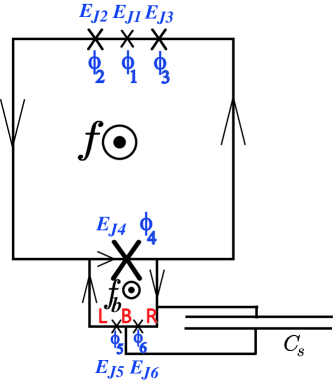
Figure 1: Flux qubit with a large Josephson junction of Josephson coupling energy $E_{J4}$. A Cooper pair box with a large shunted capacitance $C_{s}$ (transmon) is attached to the flux qubit across the large junction.

The total energy of the system in Fig. 1 consists of the Josephson junction energy and the charging energy, neglecting small inductive energy. The Josephson junction energy $U_{\rm JJ}(\{\phi_{i}\})$ is represented in terms of the phase differences $\phi_{i}$ across the Josephson junctions,

$$U_{\rm JJ}(\{\phi_{i}\})=-\sum^{6}_{i=1}E_{Ji}\cos\phi_{i}.$$ (1)

We have two boundary conditions for the upper and lower loops,

$$\phi_{1}+\phi_{2}+\phi_{3}+\phi_{4}=2\pi(n_{a}+f),$$ (2)

$$\phi_{4}+\phi_{5}+\phi_{6}=2\pi(n_{b}-f_{b})$$ (3)

with integers $n_{a}$ and $n_{b}$. Here, $f=\Phi_{\rm ext,a}/\Phi_{0}$ and $f_{b}=\Phi_{\rm ext,b}/\Phi_{0}$ with the external fluxes $\Phi_{\rm ext,a}$ and $\Phi_{\rm ext,b}$ threading the upper and lower loop, respectively, and $\Phi_{0}=h/2e$. We, for simplicity, set

$$E_{J2}=E_{J3}\equiv E_{J},~{}~{}~{}E_{J5}=E_{J6}\equiv E_{Jb},$$ (4)

and thus we have

$$\phi_{2} = \phi_{3}+2\pi m_{a},$$ (5)

$$\phi_{5} = \phi_{6}+2\pi m_{b}$$ (6)

with integers $m_{a}$ and $m_{b}$. Hereafter, we set $E_{J1}=0.8E_{J}$.

Since we have 4 constraints of Eqs. (2)-(6), the Josephson junction energy in Eq. (1) can be represented in the plane of $(\phi_{a},\phi_{b})$ as shown in Fig. 2, where

$$\phi_{a} \equiv (\phi_{2}+\phi_{3})({\rm mod}~{}2\pi)/2,$$ (7)

$$\phi_{b} \equiv (\phi_{5}+\phi_{6})({\rm mod}~{}2\pi)/2.$$ (8)

In Fig. 2, we set $f=0.5$ and $f_{b}=0.5$, and $|\downarrow\rangle$ ($|\uparrow\rangle$) denotes the counter-clockwise (clockwise) current state in the upper loop. We can observe that the current directions of upper and lower loops are correlated with each other. When $\phi_{a}>0(\phi_{a}<0),~{}\phi_{b}>0(\phi_{b}<0)$, which means, depending on the current direction in the upper loop, the sign of phase shift across the junctions 5, 6 changes. Then we can set

$$\phi_{5}({\rm mod}~{}2\pi)=\phi_{6}({\rm mod}~{}2\pi)=\pm\phi/2$$ (9)

for $|\downarrow\rangle~{}(|\uparrow\rangle)$ state with $\phi\equiv 2|\phi_{b}|$.

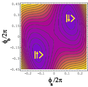
Figure 2: The Josephson junction energy $U_{\rm JJ}(\{\phi_{i}\})$ in the plane of $(\phi_{a},\phi_{b})$, where $\phi_{a}=(\phi_{2}+\phi_{3})({\rm mod}~{}2\pi)/2$ and $\phi_{b}=(\phi_{5}+\phi_{6})({\rm mod}~{}2\pi)/2$. At the local minima of $U_{\rm JJ}$, $\phi_{a}$ and $\phi_{b}$ have the same sign. For the flux state $|\downarrow\rangle$, the persistent current in the upper (lower) loop is counter-clockwise (clockwise) as shown in Fig. 1, and vice-versa for $|\uparrow\rangle$.

On the other hand, the transmon qubit states are described by the number of Copper pairs, $|n\rangle$ and $|n+1\rangle$, in the Cooper pair box (denoted as B in Fig. 1). The charging energy splitting Makhlin is given by

$$E_{n+1}-E_{n}=2E_{\rm ch}=-4E_{C}(1-2n_{g})$$ (10)

with the charging energy $E_{C}=(2e)^{2}/2C_{\Sigma}$ of the transmon and the dimensionless gate voltage $n_{g}=C_{g}V_{g}/2e$. Here, $V_{g}$ is the gate voltage and $C_{\Sigma}=C_{g}+C_{J}+C_{s}$ with the gate capacitance $C_{g}$ and the Josephson junction capacitance $C_{J}$ for transmon. The transition between the states $|n\rangle$ and $|n+1\rangle$ is invoked by the Josephson junction energy $E_{Jb}$ charge ; Makhlin .

The Hamiltonian $H_{0}$ for our qubit with $f\approx 0.5$ and $f_{b}\approx 0.5$ is given by

$$H_{0}\! = \!I\otimes[-E_{\rm ch}|B\rangle\langle B|+E_{\rm ch}(|L\rangle\langle L|+|R\rangle\langle R|)]$$

$$\!\!+(-\epsilon|\downarrow\rangle\langle\downarrow|+\epsilon|\uparrow\rangle\langle\uparrow|-\Delta|\downarrow\rangle\langle\uparrow|-\Delta|\uparrow\rangle\langle\downarrow|)\otimes I$$

$$\!\!-|\downarrow\rangle\langle\downarrow|\otimes\frac{E_{Jb}}{2}\left(e^{\frac{i}{2}\phi}|R\rangle\langle B|+e^{\frac{i}{2}\phi}|B\rangle\langle L|+c.c.\right)$$

$$\!\!-|\uparrow\rangle\langle\uparrow|\otimes\frac{E_{Jb}}{2}\left(e^{-\frac{i}{2}\phi}|R\rangle\langle B|+e^{-\frac{i}{2}\phi}|B\rangle\langle L|+c.c.\right).$$

The first term shows the energy levels of the Cooper pair box. When an additional Cooper pair is in the box, the state is represented as $|B\rangle$, while if the Cooper pair tunnels into left or right side of the box, the state is denoted as $|L\rangle$ or $|R\rangle$. For the state $|B\rangle$, the number of Cooper pairs in the box is $n+1$, while for the states $|L\rangle$ and $|R\rangle$ it is $n$. The second term describes the dynamics of the flux qubit, where $\Delta$ is the transition rate between $|\downarrow\rangle$ and $|\uparrow\rangle$, and $\epsilon=\Phi_{0}I_{p}\delta f$ is the energy level shift of flux qubit part with $\delta f=f-0.5$ and $I_{p}$ being the persistent current in the flux qubit loop. The latter two terms describe the tunneling of a Cooper pair. The phase shifts involved in the tunneling have different signs depending on the flux qubit states.

We consider the case that $E_{J4}\gg E_{Ji}$ similarly to the quantronium qubit Vion . As a result, $\phi_{4}$ is very small compared to other $\phi_{i}$’s, which allows an analytic analysis for $H_{0}$. Then, from the boundary condition of Eq. (3) around the lower loop, we obtain $\phi\approx\pi$ for $f_{b}=0.5$. If we set $\phi=\pi$, we can obtain the eigenvalues of the Hamiltonian $H_{0}$ as

$$\lambda_{0,1,2,3} = \pm\sqrt{F\pm 2\sqrt{G}},$$ (12)

$$\lambda_{4,5} = \pm\sqrt{\Delta^{2}+\epsilon^{2}}/2$$ (13)

with $F=\epsilon^{2}+\Delta^{2}+E_{\rm ch}^{2}+E^{2}_{Jb}/2$ and $G=\epsilon^{2}E_{\rm ch}^{2}+E_{\rm ch}^{2}\Delta^{2}+\epsilon^{2}E^{2}_{Jb}/2$.

For an analytic analysis we set $\epsilon=0~{}(f=0.5)$. Then the eigenstates becomes

$$|\psi_{0}\rangle = N_{0}\left[\frac{2i}{E_{Jb}}\left(\frac{1}{\sqrt{2}}Q_{+}+\Delta_{+}\right)(|\downarrow\rangle+|\uparrow\rangle)|B\rangle\right.$$ (14)

$$+(|\downarrow\rangle-|\uparrow\rangle)(|L\rangle-|R\rangle)],$$

$$|\psi_{1}\rangle = N_{1}\left[\frac{2i}{E_{Jb}}\left(\frac{1}{\sqrt{2}}Q_{-}-\Delta_{-}\right)(|\downarrow\rangle-|\uparrow\rangle)|B\rangle\right.$$ (15)

$$+(|\downarrow\rangle+|\uparrow\rangle)(|L\rangle-|R\rangle)],$$

$$|\psi_{2}\rangle = N_{2}\left[-\frac{2i}{E_{Jb}}\left(\frac{1}{\sqrt{2}}Q_{-}+\Delta_{-}\right)(|\downarrow\rangle-|\uparrow\rangle)|B\rangle\right.$$ (16)

$$+(|\downarrow\rangle+|\uparrow\rangle)(|L\rangle-|R\rangle)],$$

$$|\psi_{3}\rangle = N_{3}\left[-\frac{2i}{E_{Jb}}\left(\frac{1}{\sqrt{2}}Q_{+}-\Delta_{+}\right)(|\downarrow\rangle+|\uparrow\rangle)|B\rangle\right.$$ (17)

$$+(|\downarrow\rangle-|\uparrow\rangle)(|L\rangle-|R\rangle)].$$

with normalization factors $N_{i}$ and eigenvalues

$$\lambda_{0} = -\frac{1}{\sqrt{2}}Q_{+},\lambda_{1}=-\frac{1}{\sqrt{2}}Q_{-},$$ (18)

$$\lambda_{2} = \frac{1}{\sqrt{2}}Q_{-},\lambda_{3}=\frac{1}{\sqrt{2}}Q_{+},$$ (19)

and

$$Q_{\pm} \equiv \sqrt{E^{2}_{Jb}+2\Delta_{\pm}^{2}},$$ (20)

$$\Delta_{\pm} \equiv \Delta\pm|E_{\rm ch}|.$$ (21)

The excited states $|\psi_{4}\rangle,~{}|\psi_{5}\rangle$ corresponding to $\lambda_{4}=-\Delta_{-}$ and $\lambda_{5}=\Delta_{+}$ can also be obtained as

$$|\psi_{4}\rangle=\frac{1}{\sqrt{2}}(|\downarrow\rangle+|\uparrow\rangle)(|L\rangle+|R\rangle),$$ (22)

$$|\psi_{5}\rangle=\frac{1}{\sqrt{2}}(|\downarrow\rangle-|\uparrow\rangle)(|L\rangle+|R\rangle).$$ (23)

In the eigenstates $|\psi_{0}\rangle,|\psi_{1}\rangle,|\psi_{2}\rangle$ and $|\psi_{3}\rangle$, the flux states, $|\downarrow\rangle+|\uparrow\rangle$ and $|\downarrow\rangle-|\uparrow\rangle$, and the charge state, $|B\rangle$ and $|L\rangle-|R\rangle$, are entangled with each other, whereas the states, $|\psi_{4}\rangle$ and $|\psi_{5}\rangle$, are product state.

In Fig. 3(a) we plot four eigenvalues $\lambda_{0},~{}\lambda_{1},~{}\lambda_{2},~{}\lambda_{3}$ in the plane of $(f,n_{g})$. Here we use $E_{J}/E_{C}=100$ for transmon. Figs. 3(b) and (c) show the cut view of Fig. 3(a) along $f$ with $n_{g}=0.5$ and along $n_{g}$ with $f=0.5$, respectively. Here, the point $(f,n_{g})=(0.5,0.5)$ is an extreme point. At this point the states are degenerate and we will define the superposition of these degenerate states as a qubit state later.

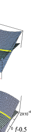
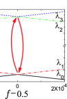
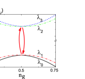
Figure 3: (a) Qubit energy levels, $\lambda_{0},\lambda_{1},\lambda_{2}$ and $\lambda_{3}$ with $\Delta/E_{J}=0.001$, $E_{Jb}/E_{J}=0.1$ and $E_{J4}/E_{J}=50$. The Rabi oscillation is performed between the local extreme points of energy planes. Cut views of (a) with (b) $n_{g}=0.5$ and (c) $f=0.5$.

The Rabi oscillation between the eigenstates can be performed by applying a magnetic microwave field $\epsilon_{\omega}(t)=g\cos\omega t$ on the qubit, where $g$ is the coupling strength between the qubit and the microwave. The total Hamiltonian is given by $H=H_{0}+H_{\rm mw}$, where $H_{\rm mw}$ describes the interaction between the qubit and the microwave,

$$H_{\rm mw}=(-\epsilon_{\omega}(t)|\downarrow\rangle\langle\downarrow|+\epsilon_{\omega}(t)|\uparrow\rangle\langle\uparrow|)\otimes I.$$ (24)

We transform the total Hamiltonian $H$ to ${\tilde{H}}$ in the basis $\{|\psi_{0}\rangle,|\psi_{1}\rangle,|\psi_{2}\rangle,|\psi_{3}\rangle,|\psi_{4}\rangle,|\psi_{5}\rangle\}$ as,

$${\tilde{H}}\!\!=\!\!\!\left(\begin{array}[]{cccccc}\!\!\!\!-\frac{1}{\sqrt{2}}Q_{+}&\!\!\!\!-g_{1}\cos\omega t&\!\!\!\!g_{2}\cos\omega t&\!\!\!\!0&\!\!\!\!\!\!0&\!\!\!\!0\\ \!\!-g_{1}\cos\omega t&\!\!\!\!-\frac{1}{\sqrt{2}}Q_{-}&\!\!\!\!0&\!\!\!\!-g_{2}\cos\omega t&\!\!\!\!\!\!0&\!\!\!\!0\\ \!\!g_{2}\cos\omega t&\!\!\!\!0&\!\!\!\!\frac{1}{\sqrt{2}}Q_{-}&\!\!\!\!-g_{1}\cos\omega t&\!\!\!\!\!\!0&\!\!\!\!0\\ \!\!\!\!0&\!\!\!\!\!\!\!\!-g_{2}\cos\omega t&\!\!\!\!-g_{1}\cos\omega t&\!\!\!\!\frac{1}{\sqrt{2}}Q_{+}&\!\!\!\!\!\!0&\!\!\!\!0\\ \!\!\!\!0&\!\!\!\!0&\!\!\!\!0&\!\!\!\!0&\!\!\!\!\!\!\!\!-\Delta_{-}&\!\!\!\!0\\ \!\!\!\!0&\!\!\!\!0&\!\!\!\!0&\!\!\!\!0&\!\!\!\!\!\!0&\!\!\!\!\!\Delta_{+}\end{array}\right)\!\!,$$ (31)

with

$$g_{1} = \frac{2\sqrt{2}\Delta+Q_{-}+Q_{+}}{2\sqrt{Q_{+}Q_{-}}}\sqrt{\frac{Q_{-}-\sqrt{2}\Delta_{-}}{Q_{+}+\sqrt{2}\Delta_{+}}}g,$$ (33)

$$g_{2} = \frac{2\sqrt{2}\Delta-Q_{-}+Q_{+}}{2\sqrt{Q_{+}Q_{-}}}\sqrt{\frac{Q_{-}+\sqrt{2}\Delta_{-}}{Q_{+}+\sqrt{2}\Delta_{+}}}g.$$ (34)

Since the states, $|\psi_{4}\rangle,|\psi_{5}\rangle$, are decoupled from the other states in ${\tilde{H}}$, we hereafter truncate these states from the basis $\{|\psi_{0}\rangle,|\psi_{1}\rangle,|\psi_{2}\rangle,|\psi_{3}\rangle,|\psi_{4}\rangle,|\psi_{5}\rangle\}$ and represent the Hamiltonian matrix ${\tilde{H}}$ in the basis $\{|\psi_{0}\rangle,|\psi_{1}\rangle,|\psi_{2}\rangle,|\psi_{3}\rangle\}$.

In order to obtain the transition probability, we introduce a rotating frame such that $\phi(t)={\cal D}\psi(t)$. Then the Schrödinger equation ${\tilde{H}}\psi(t)=i\hbar\frac{\partial}{\partial t}\psi(t)$ is written as $i\frac{\partial}{\partial t}\phi(t)=\tilde{H}^{R}\phi(t)$ with

$$\tilde{H}^{R}={\cal D}{\tilde{H}}{\cal D}^{\dagger}-i{\cal D}\frac{\partial}{\partial t}{\cal D}^{\dagger}.$$ (35)

We can choose the transition matrix ${\cal D}$ between ${\cal D}_{1}$ and ${\cal D}_{2}$,

$${\cal D}_{1}\!\!=\!\!\left(\begin{array}[]{cccc}e^{-i\omega t}&0&0&0\\ 0&1&0&0\\ 0&0&1&0\\ 0&0&0&e^{i\omega t}\end{array}\right),{\cal D}_{2}\!\!=\!\!\left(\begin{array}[]{cccc}1&0&0&0\\ 0&e^{-i\omega t}&0&0\\ 0&0&e^{i\omega t}&0\\ 0&0&0&1\end{array}\right).$$ (44)

By choosing ${\cal D}_{1}$(${\cal D}_{2}$), we can calculate the transition probability between the states $|\psi_{0}\rangle$ and $|\psi_{3}\rangle$ ($|\psi_{1}\rangle$ and $|\psi_{2}\rangle$). The Hamiltonian $\tilde{H}^{R}$ for the transition between $|\psi_{0}\rangle$ and $|\psi_{3}\rangle$ becomes

$$\!\!\!\!\!\!\tilde{H}^{R}=$$ (45)

$$\!\!\!\!\!\!\!\!\!\left(\begin{matrix}\!\!\!\!-\frac{1}{\sqrt{2}}Q_{+}\!\!+\!\omega&\!\!\!\!\!\!-\frac{g_{1}}{2}(1+e^{-2i\omega t})&\!\frac{g_{2}}{2}(1+e^{-2i\omega t})&\!\!\!\!0\cr\!\!-\frac{g_{1}}{2}(1+e^{2i\omega t})&\!\!\!\!-\frac{1}{\sqrt{2}}Q_{-}&\!\!\!\!\!\!\!\!\!\!\!\!\!0&\!\!\!\!\!\!\!\!\!\!\!\!\!\!\!\!\!\!-\frac{g_{2}}{2}(1+e^{-2i\omega t})\cr\frac{g_{2}}{2}(1+e^{2i\omega t})&\!\!\!\!0&\!\!\!\!\!\!\!\!\!\!\!\!\!\!\!\!\frac{1}{\sqrt{2}}Q_{-}&\!\!\!\!\!\!\!\!\!\!\!\!\!\!\!\!\!\!\!-\frac{g_{1}}{2}(1+e^{-2i\omega t})\cr\!\!\!\!0&\!\!\!\!\!\!\!\!\!\!\!-\frac{g_{2}}{2}(1+e^{2i\omega t})&\!\!\!\!\!\!\!\!-\frac{g_{1}}{2}(1+e^{2i\omega t})&\!\!\!\!\frac{1}{\sqrt{2}}Q_{+}\!\!-\!\omega\end{matrix}\!\!\right).$$

Here, note that the Rabi oscillation can be performed by the resonant microwave with the frequency

$$\omega=\frac{1}{\sqrt{2}}Q_{+},$$ (46)

not $2\times\frac{1}{\sqrt{2}}Q_{+}$.

At the operating point ($f,n_{g})=(0.5,0.5)$ the Rabi oscillation between $|\psi_{0}\rangle$ and $|\psi_{3}\rangle$ may be analyzed in the rotating wave approximation (RWA). The usual RWA neglects fast oscillating mode, so we set $e^{\pm 2i\omega t}=1$ in the Hamiltonian ${\tilde{H}}^{R}$ RWA . At this point, $Q_{+}=Q_{-}$, thus the eigenvalues are degenerated and the transition amplitudes are reduced as

$$g_{1} = \frac{\sqrt{2}\Delta}{\sqrt{2\Delta^{2}+E^{2}_{Jb}}}g,$$ (47)

$$g_{2} = \frac{E_{Jb}}{\sqrt{2\Delta^{2}+E^{2}_{Jb}}}g.$$ (48)

We found that for $g_{1}=g_{2}$, i.e., $E_{Jb}=\sqrt{2}\Delta$, and $g\ll\omega$, the initial state $\phi(0)=(1,0,0,0)$ evolves such that

$$e^{-i\tilde{H}^{R}t}\phi(0)=(\cos\frac{2g^{2}_{1}}{\omega}t,0,0,\sin\frac{2g^{2}_{1}}{\omega}t),$$ (49)

which shows a Rabi oscillation between $|\psi_{0}\rangle$ and $|\psi_{3}\rangle$ with the Rabi frequency

$$\Omega_{R}=\frac{4g^{2}_{1}}{\omega_{0}}$$ (50)

and

$$\omega_{0}=\frac{1}{\sqrt{2}}Q_{+}=\sqrt{\frac{E^{2}_{Jb}}{2}+\Delta^{2}}.$$ (51)

In this case the Rabi oscillation demonstrates the maximum fidelity (F=1). If one of $g_{1}$ and $g_{2}$ vanishes, we were able to check that the fidelity is zero, which means that the Rabi oscillation involves two stages.

In the Hamiltonian of Eq. (45) there are two ways in which the initial state $|\psi_{0}\rangle$ evolves to the final state $|\psi_{3}\rangle$. Note that there is no direct transition amplitude between $|\psi_{0}\rangle$ and $|\psi_{3}\rangle$ states. First of all, the initial state can evolve to the final state through the intermediate level with energy $-(1/\sqrt{2})Q_{-}$. The transitions can be done by the off-diagonal terms as

$$|\psi_{0}\rangle\rightarrow|\psi_{1}\rangle\rightarrow|\psi_{3}\rangle,$$ (52)

where the first and second steps are driven by the terms $-\frac{g_{1}}{2}(1+e^{\pm 2i\omega t})$ and $-\frac{g_{2}}{2}(1+e^{\pm 2i\omega t})$ in the Hamiltonian of Eq. (45), respectively. The second way is to pass by the level with energy $(1/\sqrt{2})Q_{-}$ such that

$$|\psi_{0}\rangle\rightarrow|\psi_{2}\rangle\rightarrow|\psi_{3}\rangle,$$ (53)

where the first and second steps are driven by the terms ${\frac{g_{2}}{2}(1+e^{\pm 2i\omega t})}$ and ${-\frac{g_{1}}{2}(1+e^{\pm 2i\omega t})}$, respectively. As a consequence, the Rabi oscillation is performed in a two way double stage manner. It can easily be checked that two matrices $\tilde{H}^{R}$ describing these processes in terms of either ${\cal D}_{1}$ or ${\cal D}_{2}$ commute with each other, so the total unitary evolution is represented as the product of these two evolution matrices.

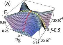
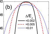
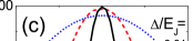
Figure 4: (a) Fidelity of Rabi oscillation with $\Delta/E_{J}=0.002$, $E_{Jb}/E_{J}=0.1$ and $E_{J4}/E_{J}=50$. Cut views of fidelity with (b) $f=0.5$ and (c) $n_{g}=0.5$.

As shown in the above evolution $e^{-i\tilde{H}^{R}t}\phi(0)$ of Eq. (49), even though the energy levels of the states $|\psi_{2}\rangle$ and $|\psi_{3}\rangle$ are degenerate for $n_{g}=0.5$, the initial state $|\psi_{0}\rangle$ always evolves to $|\psi_{3}\rangle$, not $|\psi_{2}\rangle$. Numerically also we were able to confirm the deterministic relation,

$$|\psi_{0}\rangle\rightarrow|\psi_{3}\rangle,~{}~{}~{}~{}~{}~{}~{}|\psi_{1}\rangle\rightarrow|\psi_{2}\rangle$$ (54)

through ${{\cal D}_{1}}$ and ${{\cal D}_{2}}$, respectively. This means that the Hilbert spaces spanned by the basis $\{|\psi_{0}\rangle,|\psi_{3}\rangle\}$ and by the basis $\{|\psi_{1}\rangle,|\psi_{2}\rangle\}$ are effectively decoupled.

In this case the qubit states, $|\xi_{0}\rangle$ and $|\xi_{1}\rangle$, are the superpositions of these degenerate states,

$$|\xi_{0}\rangle=\alpha|\psi_{0}\rangle+\beta|\psi_{1}\rangle,~{}~{}|\xi_{1}\rangle=\alpha|\psi_{2}\rangle+\beta|\psi_{3}\rangle.$$ (55)

The values of $\alpha$ and $\beta$ are determined when the qubit states are prepared. A Rabi pulse generates a superposition between the qubit state,

$$|\Psi(0)\rangle=p|\xi_{0}\rangle+q|\xi_{1}\rangle.$$ (56)

We checked numerically that the single qubit phase evolution can be achieved by the Larmour precession,

$$|\Psi(t)\rangle=e^{i\theta}p|\xi_{0}\rangle+e^{-i\theta}q|\xi_{1}\rangle.$$ (57)

The single qubit Rabi oscillation can also be demonstrated. In Fig. 4 (a) we plot the fidelity of the Rabi oscillation with the initial state $|\Psi(0)\rangle=|\xi_{0}\rangle$,where the fidelity is defined as the overlap $F=|\langle\Psi(\Omega_{R}t=\pi)|\xi_{1}\rangle|^{2}.$ Here we fix the resonant frequency $\omega=Q_{+}/\sqrt{2}=\omega_{0}$ as in Eq. (46). The Rabi oscillation frequency is numerically obtained as $\Omega_{R}/2\pi\approx$ 70MHz for $\Delta/E_{J}$=0.01 and $g/E_{J}$=0.05 with $E_{J}/h$=100GHz. At the operation point $(f,n_{g})=(0.5,0.5)$, the fidelity error $\delta F=1-F\sim{\rm O}(10^{-3})$ for $\Delta/E_{J}$=0.005, which is sufficiently small.

Figures 4 (b) and (c) are cut view of Fig. 4 (a). In Fig. 4 (b) the peak width is much broad because the Cooper pair box is the transmon, while the peak width at $F=0.99$ in Fig. 4 (c) is $\delta f\sim 5\times 10^{-5}$ for $\Delta/E_{J}$=0.002. Flux fluctuation is estimated to be $\sim 10^{-6}[\Phi_{0}/{\rm Hz}^{1/2}]$ Yoshi ; Bertet and flux amplitude can be controlled up to the accuracy of $10^{-5}\Phi_{0}$. Hence both the peak widths are sufficiently large. The fidelities are higher for smaller value of $\Delta/E_{Jb}$ in numerical calculation, whereas F has maximum at $E_{Jb}=\sqrt{2}\Delta$ in the RWA. The reason for this discrepancy is that the oscillating term as well as the constant term in ($1+e^{\pm 2i\omega t}$) in ${\tilde{H}}^{R}$ contributes to the transition through the intermediate level. Even for the parameter regime where the RWA works well such that $g/E_{J}=0.001\ll\omega$, the fidelities $F_{\rm RWA}$ from the RWA and $F_{\bf n}$ from the numerical calculation are different from each other; we have, for example, $(F_{\rm RWA},F_{\bf n})=(0.735,0.848),(0.889,0.782),~{}{\rm and}~{}(0.973,0.713)$ for $\Delta/E_{J}=0.04,0.05,~{}{\rm and}~{}0.06$, respectively, with $E_{J4}/E_{J}=0.1$.

III Qubit state readout

The flux qubit state has usually been detected by using the superconducting quantum interference device (SQUID). The SQUID with resistively shunted Josephson junction is biased by a current a little below the critical current so that depending on the flux qubit state the SQUID turns into voltage state to produce the readout result, giving rese to decoherence due to the backaction to the qubit state. The dispersive readout scheme with the non-linear Josephson resonator reduces the backaction and thus enables the non-destructive measurement. For the transmon qubit the single-shot readout has been performed through the dispersive measurement schemes.

For our qubit, which is a hybrid of the flux qubit and the transmon, the flux state can be read out by detecting the state of transmon. Hence, in the present scheme the non-destructive single-shot readout can be achieved by using the dispersive measurement schemes such as the Josephson bifurcation amplifier and the Josephson parametric amplifier. Owing to the large shunted capacitance the transmon is robust against the charge fluctuation, whereas the qubit operation time becomes long due to the flat energy band. Since in our study the transmon is not used as a qubit, rather as an auxiliary readout element, the qubit operation time is determined by the characteristics of the flux qubit part. Hence, our qubit readout design has the advantage of increasing the transmon capacitance sufficiently, not worrying about long qubit-operation time.

We can observe in Eqs. (14)-(17) that the qubit states $|\psi_{i}\rangle$ do not have definite magnetic moment or charge number. At the operating point $n_{g}=0.5$, $|\psi_{0}\rangle$ and $|\psi_{3}\rangle$ in Eqs. (14) and (17) approaches the states,

$$|\psi_{0}\rangle=\frac{1}{\sqrt{2}}\frac{|\downarrow\rangle-|\uparrow\rangle}{\sqrt{2}}\frac{|L\rangle-|R\rangle}{\sqrt{2}}+\frac{i}{\sqrt{2}}\frac{|\downarrow\rangle+|\uparrow\rangle}{\sqrt{2}}|B\rangle,$$ (58)

$$|\psi_{3}\rangle=\frac{1}{\sqrt{2}}\frac{|\downarrow\rangle-|\uparrow\rangle}{\sqrt{2}}\frac{|L\rangle-|R\rangle}{\sqrt{2}}-\frac{i}{\sqrt{2}}\frac{|\downarrow\rangle+|\uparrow\rangle}{\sqrt{2}}|B\rangle,$$

as $\Delta/E_{Jb}$ decreases. For both states the probability for having an additional Cooper pair is 0.5, which means we cannot discriminate between $|\psi_{0}\rangle$ and $|\psi_{3}\rangle$ through charge detection.

In order to read out the qubit state, we apply an oscillating electric field on the qubit,

$$H_{\rm osc}=I\otimes g_{e}\cos\omega_{e}t[-(|L\rangle\langle L|+|R\rangle\langle R|)+|B\rangle\langle B|].$$ (59)

In the basis $\{|\psi_{0}\rangle,|\psi_{1}\rangle,|\psi_{2}\rangle,|\psi_{3}\rangle\}$, the transformed Hamiltonian ${\tilde{H}}_{\rm osc}$ is represented as

$$\tilde{H}_{\rm osc}\!=g_{e}\cos\omega_{e}t\!\left(\begin{array}[]{cccc}\frac{\sqrt{2}\Delta_{+}}{Q_{+}}&0&0&-\frac{E_{Jb}}{Q_{+}}\\ 0&-\frac{\sqrt{2}\Delta_{-}}{Q_{-}}&-\frac{E_{Jb}}{Q_{-}}&0\\ 0&-\frac{E_{Jb}}{Q_{-}}&\frac{\sqrt{2}\Delta_{-}}{Q_{-}}&0\\ -\frac{E_{Jb}}{Q_{+}}&0&0&-\frac{\sqrt{2}\Delta_{+}}{Q_{+}}\end{array}\right)\!\!.$$ (64)

Since $\tilde{H}_{0}$ in this basis is diagonal, the total Hamiltonian $H_{\rm read}=H_{0}+H_{\rm osc}$ is transformed to a direct sum of $2\times 2$ matrices,

$$\tilde{H}_{\rm read}=\tilde{H}^{1}_{\rm read}\oplus\tilde{H}^{2}_{\rm read},$$ (65)

where the basis is $\{|\psi_{0}\rangle,|\psi_{3}\rangle\}$ for $\tilde{H}^{1}_{\rm read}$ and $\{|\psi_{1}\rangle,|\psi_{2}\rangle\}$ for $\tilde{H}^{2}_{\rm read}$. By a proper rotation in the $2\times 2$ subspace the qubit state can be transformed to a state which have a definite charge number.

For an analytic analysis we consider $n_{g}=0.5~{}(E_{\rm ch}=0)$ and negligible $\Delta/E_{Jb}$, then

$$\tilde{H}^{1}_{\rm read}=\tilde{H}^{2}_{\rm read}=-\frac{E_{Jb}}{\sqrt{2}}\sigma_{z}-g_{e}\cos\omega_{e}t\sigma_{x}.$$ (66)

The transition between $\{|\psi_{0}\rangle,|\psi_{3}\rangle\}$ is described by $\tilde{H}^{1}_{\rm read}$. In a rotating frame the Hamiltonian $\tilde{H}^{1,{\rm R}}_{\rm read}$ is given by Eq. (35) with ${\cal D}=e^{i\sigma_{z}\omega_{e}t}$. Further, in the RWA the fast oscillating modes are neglected as $e^{\pm i\omega_{e}t}=1$, resulting in

$$\tilde{H}^{1,{\rm R}}_{\rm read}=\left(\begin{array}[]{cc}-\frac{E_{Jb}}{\sqrt{2}}+\frac{\omega_{e}}{2}&-\frac{g_{e}}{2}\\ -\frac{g_{e}}{2}&\frac{E_{Jb}}{\sqrt{2}}-\frac{\omega_{e}}{2}\end{array}\right).$$ (69)

If we set $\omega_{e}$ resonant with the qubit energy gap

$$\omega_{e}=2\times E_{Jb}/\sqrt{2},$$ (70)

by using the time evolution of the qubit state $|\psi(t)\rangle=e^{-i\tilde{H}^{1,{\rm R}}_{\rm read}t}|\psi(0)\rangle$ the evolutions of initial states $|\psi_{0}(0)\rangle_{R}$ and $|\psi_{3}(0)\rangle_{R}$ in the rotating frame after $\pi/2$-rotation ($g_{e}\tau_{r}=\pi/2$) are given by

$$|\psi_{0}(0)\rangle_{R}=\left(\begin{array}[]{c}1\\ 0\end{array}\right)\longrightarrow|\psi_{0}(\pi/2)\rangle_{R}=\frac{1}{\sqrt{2}}\left(\begin{array}[]{c}1\\ i\end{array}\right),$$ (75)

$$|\psi_{3}(0)\rangle_{R}=\left(\begin{array}[]{c}0\\ 1\end{array}\right)\longrightarrow|\psi_{3}(\pi/2)\rangle_{R}=\frac{1}{\sqrt{2}}\left(\begin{array}[]{c}i\\ 1\end{array}\right).$$ (80)

If the condition $\omega_{e}\tau_{r}=2\pi(p-1/4)$ with integer $p$ is satisfied, the final states in laboratory frame, $|\psi\rangle=e^{i\sigma_{z}\omega_{e}t}|\psi\rangle_{R}$, have definitely different charge numbers as follows,

$$|\psi_{0}\left(\frac{\pi}{2}\right)\rangle = \frac{1-i}{2}(|\psi_{0}(0)\rangle-|\psi_{3}(0)\rangle)$$ (81)

$$= \frac{1+i}{\sqrt{2}}\frac{|\downarrow\rangle+|\uparrow\rangle}{\sqrt{2}}|B\rangle,$$

$$|\psi_{3}\left(\frac{\pi}{2}\right)\rangle = \frac{1+i}{2}(|\psi_{0}(0)\rangle+|\psi_{3}(0)\rangle)$$ (82)

$$= \frac{1+i}{\sqrt{2}}\frac{|\downarrow\rangle-|\uparrow\rangle}{\sqrt{2}}\frac{|L\rangle\!-\!|R\rangle}{\sqrt{2}},$$

where $|\psi_{0}(0)\rangle$, $|\psi_{3}(0)\rangle$ are $|\psi_{0}\rangle$, $|\psi_{3}\rangle$ in Eq. (58), respectively. This condition with $p=10$ and $g_{e}\tau_{r}=\pi/2$ implies that the coupling constant should be adjusted as $g_{e}\approx 360$MHz with $E_{Jb}=0.1E_{J}$ and $E_{J}$=100GHz. We also carry out the analysis for the transition between $\{|\psi_{1}\rangle,|\psi_{2}\rangle\}$ described by $\tilde{H}^{2}_{\rm read}$, resulting in

$$|\psi_{1}(\frac{\pi}{2})\rangle = \frac{1-i}{2}(|\psi_{1}(0)\rangle-|\psi_{2}(0)\rangle)$$ (83)

$$= \frac{1+i}{\sqrt{2}}\frac{|\downarrow\rangle-|\uparrow\rangle}{\sqrt{2}}|B\rangle,$$

$$|\psi_{2}(\frac{\pi}{2})\rangle = \frac{1+i}{2}(|\psi_{1}(0)\rangle+|\psi_{2}(0)\rangle)$$ (84)

$$= \frac{1+i}{\sqrt{2}}\frac{|\downarrow\rangle\!+\!|\uparrow\rangle}{\sqrt{2}}\frac{|L\rangle\!-\!|R\rangle}{\sqrt{2}}.$$

If we change the basis into the Cooper pair number state,

$$|n+1\rangle=|B\rangle,~{}~{}|n\rangle=\frac{|L\rangle-|R\rangle}{\sqrt{2}},$$ (85)

the qubit states of Eq. (55) are written as

$$|\xi_{0}\!\!\left(\frac{\pi}{2}\right)\rangle \!\!=\!\! \left[\frac{\alpha}{\sqrt{2}}(|\downarrow\rangle+|\uparrow\rangle)+\frac{\beta}{\sqrt{2}}(|\downarrow\rangle-|\uparrow\rangle)\right]|n+1\rangle,$$

$$|\xi_{1}\!\!\left(\frac{\pi}{2}\right)\rangle \!\!=\!\! \left[\frac{\alpha}{\sqrt{2}}(|\downarrow\rangle+|\uparrow\rangle)+\frac{\beta}{\sqrt{2}}(|\downarrow\rangle-|\uparrow\rangle)\right]|n\rangle.$$ (86)

Figure 5: Readout fidelity $F$ of the state $|\xi_{0}(\pi/2)\rangle$ after $\pi/2$-rotation. Here, $E_{Jb}/E_{J}=0.1$ and $E_{J4}/E_{J}=50$.

In this case the readout fidelity is defined as the overlap with the number state,

$$F=|\langle\xi_{0}\left(\frac{\pi}{2}\right)|n+1\rangle|^{2}~{}~{}{\rm or}~{}~{}F=|\langle\xi_{1}\left(\frac{\pi}{2}\right)|n\rangle|^{2}.$$ (87)

In Fig. 5 we show the numerical results for the fidelity $F$ of $|\xi_{0}(\pi/2)\rangle$ state, where the fidelity error $\delta F=1-F$ is as much small as $\delta F\sim{\rm O}(10^{-4})$ for $\Delta/E_{J}=0.001$. Non-destructive single-shot charge detection can be performed by the dispersive measurement using the non-linear Josephson resonator Mallet ; Vijay which has the advantages of high speed and sensitivity, low backaction, and the absence of on-chip dissipation.

We employed the special conditions $g_{e}\tau_{r}=\pi/2$ and $\omega_{e}\tau_{r}=2\pi(p-1/4)$ for charge detection. However, the general conditions for qubit state readout are given by

$$g_{e}\tau_{r}=2\pi q\pm\pi/2,$$ (88)

$$\omega_{e}\tau_{r}=2\pi p\pm\pi/2$$ (89)

with integers $p,q$. These conditions result in the relation between the coupling constant $g_{e}$ and the Josephson coupling energy $E_{Jb}$ as follows,

$$g_{e}=\frac{4q\pm 1}{4p\pm 1}\sqrt{2}E_{Jb}.$$ (90)

With $(4q+1,4p-1)$ or $(4q-1,4p+1)$ in Eq. (90), we have the charge states $|\psi_{0,1}(\pi/2)\rangle\sim|n+1\rangle$ and $|\psi_{2,3}(\pi/2)\rangle\sim|n\rangle$, whereas with $(4q+1,4p+1)$ or $(4q-1,4p-1)$ we have $|\psi_{0,1}(\pi/2)\rangle\sim|n\rangle$ and $|\psi_{2,3}(\pi/2)\rangle\sim|n+1\rangle$. In this study we use the parameter value, $E_{Jb}/E_{J}$=0.1. Hence, the coupling strength $g_{e}$ is estimated as $g_{e}\sim$ 10GHz for $p=q$ with $E_{J}$=100GHz, which is too strong to be realizable. In order to obtain a moderate coupling strength $g_{e}$ we need to adopt large $p$ and small $q$ in Eq. (90). We set $p=10$ and $q=0$, and according to Eqs. (70) and (89) we estimate the measurement time $\tau_{r}\sim$ 1 ns, which is sufficiently short to maintain qubit coherence during the measurement.

IV Discussions and Summary

The operating point $(f,n_{g})=(0.5,0.5)$ can be an optimally biased point with respect to both $f$ and $n_{g}$ for the qubit states $|\xi_{0(1)}\rangle$. The pure dephasing rate due to several fluctuating fields is given by $1/T^{*}_{2}=\sum_{i}(1/2\hbar^{2})\cos^{2}\eta_{i}S_{Xi}$ Makhlin ; Makhlin2 with the noise power $S_{Xi}$. Here $\eta_{\rm fl}=\tan^{-1}(\Delta/\epsilon)$ and $\eta_{\rm ch}=\tan^{-1}(E_{Jb}/2E_{\rm ch})$ for flux and charge fluctuation, respectively. Since $\cos\eta_{\rm fl}=0$ and $\cos\eta_{\rm ch}=0$ at the operating point $\epsilon=0$ and $E_{\rm ch}=0$, relaxation is dominant decoherence process at this optimal point. The relaxation rate is given by $1/T_{1}=\sum_{i}(1/2\hbar^{2})\sin^{2}\eta_{i}S_{Xi}$. It is known in experiments that $T_{1,{\rm fl}}\sim 1\mu$s for flux qubit flux and $T_{1,{\rm ch}}\sim 1\mu$s for transmon qubit Mallet , resulting in $T_{1}\sim 0.5\mu$s. If we increase the capacitance of the transmon in the present scheme, the relaxation rate can be decreased further. Then, the relaxation time $T_{1}$ of our qubit can approach that for the flux qubit.

For multi-qubit case the coefficients $\{\alpha^{(k)},\beta^{(k)}\}$ may be different for different qubit-$(k)$. As shown in Eq. (III), however, the states $|\xi_{0}(\pi/2)\rangle$ and $|\xi_{1}(\pi/2)\rangle$ produce definite charge detection results regardless of the values of $\alpha$ and $\beta$. Hence multi-qubit operation and readout of the qubit states can also be achieved with these qubits.

In summary, we propose a readout scheme for the superconducting flux qubit which is a hybrid of the usual three-Josephson junction qubit and the transmon. The phase degree of freedom of flux qubit loop and the charge degree of freedom of transmon are entangled with each other so that the qubit state readout can be achieved by detecting the charge number of the transmon. A $\pi/2$-rotation of the entangled state by an electric field results in the discriminating charge number state which is correlated with the current state of the flux qubit. We show that the non-destructive single-shot measurement for the flux qubit state can be achieved by detecting the state of tranmon. Further, the readout can be performed at an optimally biased point with respect to both the magnetic field and gate voltage. The fidelity of qubit state readout is shown to be sufficiently high.

ACKNOWLEDGMENTS

This research was supported by Basic Science Research Program through the National Research Foundation of Korea (NRF) funded by the Ministry of Education, Science and Technology (2011-0023467; MDK).

References

- (1) A. B. Zorin, Phys. Rev. Lett. 86, 3388 (2001).
- (2) A. Lupaşcu, C. J. M. Verwijs, R. N. Schouten, C. J. P. M. Harmans, and J. E. Mooij, Phys. Rev. Lett. 93, 177006 (2004).
- (3) I. Siddiqi, R. Vijay, F. Pierre, C. M. Wilson, M. Metcalfe, C. Rigetti, L. Frunzio, and M. H. Devoret, Phys. Rev. Lett. 93, 207002 (2004).
- (4) A. Blais, R.-S. Huang, A. Wallraff, S. M. Girvin, and R. J. Schoelkopf, Phys. Rev. A 69, 062320 (2004).
- (5) A. Wallraff, D. I. Schuster, A. Blais, L. Frunzio, J. Majer, M.H. Devoret, S. M. Girvin, and R. J. Schoelkopf, Phys. Rev. Lett. 95, 060501 (2005).
- (6) A. Blais, J. Gambetta, A. Wallraff, D. I. Schuster, S. M. Girvin, M. H. Devoret, and R. J. Schoelkopf, Phys. Rev. A 75, 032329 (2007).
- (7) I. Siddiqi, R. Vijay, M. Metcalfe, E. Boaknin, L. Frunzio, R. J. Schoelkopf, and M. H. Devoret, Phys. Rev. B 73, 054510 (2006).
- (8) A. Lupaşcu, E. F. C. Driessen, L. Roschier, C. J. P. M. Harmans, and J. E. Mooij, Phys. Rev. Lett. 96, 127003 (2006).
- (9) J. Koch, T. M. Yu, J. Gambetta, A. A. Houck, D. I. Schuster, J. Majer, A. Blais, M. H. Devoret, S. M. Girvin, and R. J. Schoelkopf, Phys. Rev. A 76, 042319 (2007)
- (10) J. Q. You, X. Hu, S. Ashhab, and F. Nori, Phys. Rev. B 75, 140515(R) (2007)
- (11) J. A. Schreier, A. A. Houck, J. Koch, D. I. Schuster, B. R. Johnson, J. M. Chow, J. M. Gambetta, J. Majer, L. Frunzio, M. H. Devoret, S. M. Girvin, and R. J. Schoelkopf, Phys. Rev B 77, 180502(R) (2008).
- (12) F. Mallet, F. R. Ong, A. Palacios-Laloy, F. Nguyen, P. Bertet, D. Vion, and D. Esteve, Nature Phys. 5, 791 (2009).
- (13) R. Vijay, D. H. Slichter, and I. Siddiqi, Phys. Rev. Lett. 106, 110502 (2011).
- (14) A. A. Houck, J. A. Schreier, B. R. Johnson, J. M. Chow, J. Koch, J. M. Gambetta, D. I. Schuster, L. Frunzio, M. H. Devoret, S. M. Girvin, and R. J. Schoelkopf, Phys. Rev. Lett. 101, 080502 (2008).
- (15) J. E. Mooij, T. P. Orlando, L. Levitov, L. Tian, C. H. van der Wal, and S. Lloyd, Science 285, 1036 (1999).
- (16) A. O. Niskanen, K. Harrabi, F. Yoshihara, Y. Nakamura, S. Lloyd, and J. S. Tsai, Science 316, 723 (2007).
- (17) T. Hime, P. A. Reichardt, B. L. T. Plourde, T. L. Robertson, C.-E. Wu, A. V. Ustinov, and J. Clarke, Science 314, 1427 (2006).
- (18) Y. Nakamura, Yu. A. Pashkin, and J. S. Tsai, Nature 398, 786 (1999).
- (19) Y. Makhlin, G. Schön, and A. Shnirman, Nature 398, 305 (1999).
- (20) Yu. A. Pashkin, T. Yamamoto, O. Astafiev, Y. Nakamura, D. V. Averin, and J. S. Tsai, Nature 421, 823 (2003).
- (21) T. Yamamoto, Yu. A. Pashkin, O. Astafiev, Y. Nakamura and J. S. Tsai, Nature 425, 941 (2003).
- (22) M. A. Sillanpää, T. Lehtinen, A. Paila, Yu. Makhlin, L. Roschier, and P. J. Hakonen, Phys. Rev. Lett. 95, 206806 (2005).
- (23) Yu. A. Pashkin, O. Astafiev, T. Yamamoto, Y. Nakamura and J. S. Tsai, Quantum Inf. Process 8, 55 (2009).
- (24) D. Vion, A. Aassime, A. Cottet, P. Joyez, H. Pothier, C. Urbina, D. Esteve, and M. H. Devoret, Science 296, 886 (2002).
- (25) N. Boulant, G. Ithier, P. Meeson, F. Nguyen, D. Vion, D. Esteve, I. Siddiqi, R. Vijay, C. Rigetti, F. Pierre, and M. Devoret, Phys. Rev. B 76, 014525 (2007).
- (26) E. Il′ichev, N. Oukhanski, A. Izmalkov, Th. Wagner, M. Grajcar, H.-G. Meyer, A. Yu. Smirnov, A. M. van den Brink, M. H. S. Amin, and A. M. Zagoskin, Phys. Rev. Lett. 91, 097906 (2003).
- (27) A. A. Abdumalikov Jr., O. Astafiev, Y. Nakamura, Y. A. Pashkin, and J. S. Tsai, Phys. Rev. B 78, 180502(R) (2008).
- (28) Y. Makhlin, G. Schön, and A. Shnirman, Rev. Mod. Phys. 73, 357 (2001).
- (29) E. T. Jaynes and F. W. Cummings, Proc. IEEE 51, 89 (1963).
- (30) F. Yoshihara, K. Harrabi, A. O. Niskanen, Y. Nakamura, and J. S. Tsai, Phys. Rev. Lett. 97, 167001 (2006).
- (31) P. Bertet, I. Chiorescu, G. Burkard, K. Semba, C. J. P. M. Harmans, D. P. DiVincenzo, and J. E. Mooij, Phys. Rev. Lett. 95, 257002 (2005).
- (32) Y. Makhlin, G. Schön, and A. Shnirman, in New Directions in Mesoscopic Physics, edited by R. Fazio, V. F. Gantmakher, and Y. Imry (Kluwer, Dordrecht, 2003).