Time-averaged MSD of Brownian motion

Abstract

We study the statistical properties of the time-averaged mean-square displacements (TAMSD). This is a standard non-local quadratic functional for inferring the diffusion coefficient from an individual random trajectory of a diffusing tracer in single-particle tracking experiments. For Brownian motion, we derive an exact formula for the Laplace transform of the probability density of the TAMSD by mapping the original problem onto chains of coupled harmonic oscillators. From this formula, we deduce the first four cumulant moments of the TAMSD, the asymptotic behavior of the probability density and its accurate approximation by a generalized Gamma distribution.

Keywords: diffusion, Brownian motion, MSD, time average, single-particle tracking

1 Introduction

The statistical properties of Brownian motion play a crucial role in disciplines as various as mathematics, physics, chemistry, biology, engineering, economics and ecology [1, 2, 3, 4, 5]. In many cases, an observation or an experiment can be repeated a large number of times to get a representative statistics of outcomes. In other situations, one measures an observable which reflects a cumulative effect of a large number of molecules (e.g., the macroscopic nuclear magnetic resonance signal formed by an extremely large number of nuclei [5]). In both cases, a system can be characterized by ensemble-averaged quantities. For instance, the ensemble average (or expectation) of the mean-square displacement (MSD) of a freely diffusing particle, $\langle X^{2}(t)\rangle$, yields a measure of the diffusion coefficient $D$ through the Einstein’s relation: $\langle X^{2}(t)\rangle=2Dt$. However, there are other situations when few or even single stochastic trajectory $X(t)$ is available that makes the ensemble averaging inaccurate or impossible. The common examples are stock prices in finance [6] or trajectories of macromolecules inside living cells acquired by single particle tracking (SPT) techniques [3, 7, 8, 9, 10, 11, 12, 13, 14, 15, 16]. In the former case, the observation (i.e., a price time series) is evidently unique for each asset. In the latter case, although an experiment can be repeated, the ensemble average may still be problematic, especially for tracers that move in spatially heterogeneous and time-evaluating media such as living cells. In order to infer the dynamical information from such individual trajectories, one needs therefore to replace ensemble averages by time averages. For instance, the diffusion coefficient is often inferred by considering the time-averaged MSD (TAMSD) at a lag time $t$ over a sample trajectory of duration $T$:

$$\chi_{t,T}=\frac{1}{T-t}\int\limits_{0}^{T-t}dt_{0}(X(t_{0}+t)-X(t_{0}))^{2}.$$ (1)

Although this is still a random variable, the time average reduces its fluctuations around the mean which, for Brownian motion, is $\langle\chi_{t,T}\rangle=2Dt$.

The statistical properties of quadratic functionals of a Gaussian process have been intensively studied. In mathematical statistics, several series representations of the probability density of a general quadratic form of a Gaussian process have been proposed, e.g. a mixture of chi-squared distributions [21, 22, 23, 24], a power series expansion [25, 26], and a series expansion over Laguerre polynomials [27, 28, 29] (see also [30, 31] for a review). For biophysical applications, Qian and co-workers analyzed the TAMSD of a discrete random walk which is known to have a Gamma (or chi-squared) distribution only at the smallest lag time [7]. The distribution of diffusion coefficients was also studied via Monte Carlo simulations by Saxton [8, 9] (see also [10, 32] for experimental data). More recently, Boyer and Dean investigated the distribution of several estimators of diffusion coefficients for Brownian motion [33]. They reduced the analysis of least-squares and maximum likelihood estimates to the distribution of a local quadratic functional of Brownian motion. Mapping this problem onto an imaginary time Schrödinger equation, they derived explicit analytical results for the distribution of the diffusion coefficient estimator. In a separate paper, Boyer and co-workers discussed the optimal way to extract diffusion coefficients from single trajectories of Brownian motion and showed the superior efficiency of the maximum likelihood estimator over least-squares estimates [34]. An optimal Bayesian method for quantifying biomolecule diffusivity was presented by Voisinne et al. [35].

A different approach to the analysis of inferring schemes with quadratic functionals was developed by Grebenkov [36, 37]. First, the explicit formulas for the mean and variance of the TAMSD (and another quadratic functional) were derived for a large class of Gaussian processes governed by a generalized Langevin dynamics [36]. The formula for the variance allows one to estimate the spread of measurements and to choose an appropriate sample duration $T$. Second, a matrix representation for the characteristic function of $\chi_{t,T}$ was used in order to analyze the probability density $p(z)$ of the TAMSD of a general discrete Gaussian process [37]. Moreover, an empirical approximation for $p(z)$ by a generalized Gamma distribution (GGD) was proposed:

$$p(z)=\frac{z^{\nu-1}}{2(ab)^{\nu/2}K_{\nu}(2\sqrt{a/b})}\exp\left(-\frac{a}{z}-\frac{z}{b}\right),$$ (2)

with three parameters $a\geq 0$, $b>0$ and $\nu\in{\mathbb{R}}$, and $K_{\nu}(z)$ is the modified Bessel function of the second kind (in the limit $a\to 0$, one retrieves the Gamma distribution $\frac{z^{\nu-1}e^{-z/b}}{\Gamma(\nu)b^{\nu}}$). Although the high accuracy of the GGD approximation (2) was confirmed numerically for a discrete Brownian motion, the theoretical status of this approximation remained unclear. In addition, the dependence of the parameters $a$, $b$ and $\nu$ on the lag time $t$ was not analyzed.

In this paper, we rigorously characterize the TAMSD of Brownian motion. In Sect. 2, we introduce a functional integral representation for a Laplace transform $\varphi(s)$ of the probability density $p(z)$ which is a cornerstone for all consecutive derivations. For $t>T/2$, it leads to a simple closed formula for $\varphi(s)$. For $t<T/2$, an exact representation of $\varphi(s)$ involves a determinant of an explicit matrix of size $[T/t]\times[T/t]$, $[T/t]$ being an integer part of $T/t$. In Sect. 3, we discuss some practical consequences of these theoretical results. In particular, we derive the explicit formulas for the first four cumulant moments of the TAMSD, as well as the asymptotic behavior of the probability density $p(z)$ at small and large $z$. For instance, we show that $p(z)$ decays as $e^{-a/z}$ at small $z$ that justifies the use of a GGD as a convenient approximation for $p(z)$. It also explains a remarkable accuracy of this approximation which correctly reproduces the asymptotic behavior of $p(z)$ at both small and large $z$. Finally, we derive the asymptotic relations for the parameters $a$, $b$ and $\nu$ of the GGD as functions of the lag time $t$ by matching the first moments of the true and approximate distributions. These relations allow one to get an accurate approximation of the probability density $p(z)$ for a given lag time $t$ that opens a number of practical applications for single-particle tracking experiments. These findings and future perspectives are summarized in Conclusion.

2 Theoretical results

Throughout this section, we consider $X(u)$ to be Brownian motion with mean zero and covariance $\langle X(u),X(v)\rangle=\min\{u,v\}$, with diffusion coefficient $D$ set to $1/2$. The sample duration $T$ is fixed to $1$, while the lag time $t\in[0,1]$ is dimensionless. We are interested in the probability density $p_{t}(z)=\langle\delta(z-\chi_{t})\rangle$ of the random variable $\chi_{t}$ which denotes the TAMSD of $X(u)$:

$$\chi_{t}=\frac{1}{1-t}\int\limits_{0}^{1-t}du(X(u+t)-X(u))^{2}.$$ (3)

We aim at calculating the Laplace transform $\varphi_{t}(s)$ of the probability density $p_{t}(z)$

$$\varphi_{t}(s)=\langle\exp(-s\chi_{t})\rangle=\int\limits_{0}^{\infty}dz\,e^{-sz}p_{t}(z),$$ (4)

Once $\varphi_{t}(s)$ is obtained, one can retrieve the probability density $p_{t}(z)$ either through the inverse Laplace transform of $\varphi_{t}(s)$, or through the inverse Fourier transform of the characteristic function $\phi_{t}(k)\equiv\langle e^{ik\chi_{t}}\rangle=\varphi_{t}(-ik)$ (although both ways are formally equivalent, Fourier transforms are more convenient for numerical implementation). From a theoretical point of view, the knowledge of $\varphi_{t}(s)$ is therefore fully equivalent to that of $p_{t}(z)$ (see Sect. 3 for practical consequences).

We start by expressing the Laplace transform in Eq. (4) as a functional integral over trajectories $X(u)$ of a Brownian motion [4, 17]

$$\varphi_{t}(s)=\int\limits_{\mathbb{R}}dx_{1}\int\limits_{X(0)=0}^{X(1)=x_{1}}\mathcal{D}X(u)\exp\left(-\frac{1}{2}\int\limits_{0}^{1}(\partial_{u}X(u))^{2}-\frac{s}{1-t}\int\limits_{0}^{1-t}(X(u+t)-X(u))^{2}\right),$$ (5)

where we assume that Brownian motion starts from the origin: $X(0)=0$ (anyway, the TAMSD is translation invariant and thus the above functional integral is independent of the starting point). The next step would be to use the Feynman-Kac formula [4, 18] and map the functional integral to a propagator of a certain quantum mechanical problem, to compute the propagator and to evaluate $\varphi_{t}(s)$. This method was successfully used by Boyer and Dean for local quadratic functionals of Brownian motion [33]. However, in our problem different parts of the trajectory, at times $u$ and $u+t$, are coupled, and the action is non-local, forbiding a direct use of the Feynman-Kac formalism. To overcome this difficulty, we partition the trajectory into pieces and relabel them as new Brownian walkers in order to reduce it to an effectively many-body but local problem. The latter is not surprising since a system with memory is often equivalent to some many-body system, for example dynamics of a classical spin-glass or quantum mean-field spin-glass are typically mapped onto single particle problems with memory [19, 20]. The transformation appearing in our problem is similar in spirit, but uses the inverse mapping to turn a non-local single particle problem into a local many-body problem. We illustrate this in detail for the case $t>\frac{1}{2}$ where the mapping and the computation are relatively simple. The case $t<\frac{1}{2}$ is a straightforward generalization which is treated in the next Subsection.

Figure 1: (Color online) Splitting of a trajectory into blocks. (a) For $t>\frac{1}{2}$, there are only three blocks: two coupled parts $Y_{0}$ and $Y_{1}$ and one free part $Z_{0}$; (b) When $t=\frac{1}{m}$ ($m=2,3,4,...$), a trajectory is split into $m$ equal blocks yielding a chain of $m$ successively coupled oscillators $Y_{0}$, …, $Y_{m-1}$; (c) When $\frac{1}{1+m}<t<\frac{1}{m}$ (for some $m=2,3,4,...$), the time interval $[0,1]$ is covered by $m$ subintervals of duration $t$, plus a smaller interval $[1-mt,1]$ of duration $\delta=1-mt$. In order to split the interval $[0,1]$ regularly, each subinterval is divided into two parts, of durations $\delta$ and $t-\delta$, respectively. As a consequence, the trajectory is mapped onto two chains of coupled oscillators $\{Y_{k}\}$ and $\{Z_{k}\}$. The two chains $\{Y_{k}\}$ and $\{Z_{k}\}$ are coupled through boundary conditions for successive parts of the trajectory: $Y_{k}(\delta)=Z_{k}(0)$, $k=0,...,m-1$ which express continuity of the original trajectory $X(u)$.

2.1 Case $t>\frac{1}{2}$

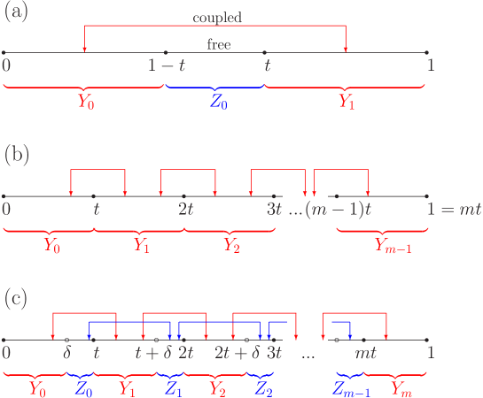
The partitioning of the trajectory in the case $t<\frac{1}{2}$ is illustrated on Fig. 1a. We split the whole trajectory $X(u)$ into three parts:

$$Y_{0}(u) = X(u)\hskip 64.01869ptu\in[0,1-t],$$

$$Z_{0}(u) = X(u+1-t)\qquad u\in[0,2t-1],$$

$$Y_{1}(u) = X(u+t)\hskip 45.5244ptu\in[0,1-t].$$

The original trajectory is then replaced by a collection of two harmonically coupled particles and a free walker. Boundary conditions express continuity of the original trajectory $X(u)$:

$$\varphi_{t}(s)=\int\limits_{{\mathbb{R}}^{3}}dx_{1-t}dx_{t}dx_{1}\int\limits_{Y_{0}(0)=0}^{Y_{0}(1-t)=x_{1-t}}\mathcal{D}Y_{0}\int\limits_{Z_{0}(0)=x_{1-t}}^{Z_{0}(2t-1)=x_{t}}\mathcal{D}Z_{0}\int\limits_{Y_{1}(0)=x_{t}}^{Y_{1}(1-t)=x_{1}}\mathcal{D}Y_{1}$$

$$\times\exp\left(-\frac{1}{2}\int\limits_{0}^{2t-1}du\,(\partial_{u}Z_{0})^{2}-\frac{1}{2}\int\limits_{0}^{1-t}du\,\left[(\partial_{u}Y_{0})^{2}+(\partial_{u}Y_{1})^{2}\right]-\frac{g^{2}}{2}\int\limits_{0}^{1-t}du\,(Y_{1}-Y_{0})^{2}\right).$$

Note that the subscripts of $x_{1-t}$, $x_{t}$ and $x_{1}$ are just notations for these integration variables. We have defined for convenience

$$g^{2}=\frac{2s}{1-t}.$$

The original non-locality is translated into harmonic coupling of particles $Y_{0}$, $Y_{1}$, the overall action is now local. Since there are just two particles involved, this case is easy to resolve: $Y_{0}$, $Y_{1}$ are decoupled in a standard way by defining their normal modes $A_{0}$, $A_{1}$

$$A_{0}(u)=\frac{1}{\sqrt{2}}(Y_{0}(u)+Y_{1}(u)),\qquad A_{1}(u)=\frac{1}{\sqrt{2}}(Y_{0}(u)-Y_{1}(u)),$$

where $A_{0}$ represents the center of mass motion and $A_{1}$ describes harmonic oscillations around the center of mass. Boundary conditions for $A_{0}$ and $A_{1}$ are:

$$a_{0,0} = A_{0}(0)=\frac{1}{\sqrt{2}}(Y_{0}(0)+Y_{1}(0))=\frac{1}{\sqrt{2}}(0+x_{t}),$$

$$a_{0,1-t} = A_{0}(1-t)=\frac{1}{\sqrt{2}}(Y_{0}(1-t)+Y_{1}(1-t))=\frac{1}{\sqrt{2}}(x_{1-t}+x_{1}),$$

$$a_{1,0} = A_{1}(0)=\frac{1}{\sqrt{2}}(Y_{0}(0)-Y_{1}(0))=\frac{1}{\sqrt{2}}(0-x_{t}),$$

$$a_{1,1-t} = A_{1}(1-t)=\frac{1}{\sqrt{2}}(Y_{0}(1-t)-Y_{1}(1-t))=\frac{1}{\sqrt{2}}(x_{1-t}-x_{1}).$$

Therefore we get a system of two free particles $Z_{0}$, $A_{0}$ and one harmonic oscillator $A_{1}$:

$$\varphi_{t}(s)=\int\limits_{{\mathbb{R}}^{3}}dx_{1-t}\,dx_{t}\,dx_{1}\int_{A_{1}(0)=a_{1,0}}^{A_{1}(1-t)=a_{1,1-t}}\mathcal{D}A_{1}\,\exp\left(-\frac{1}{2}\int_{0}^{1-t}du(\partial_{u}A_{1})^{2}-\frac{g^{2}}{2}\int_{0}^{1-t}duA_{1}^{2}\right)\times$$

$$\int_{Z(0)=x_{1-t}}^{Z(2t-1)=x_{t}}\mathcal{D}Z_{0}\exp\left(-\frac{1}{2}\int_{0}^{2t-1}du(\partial_{u}Z_{0})^{2}\right)\int_{A_{0}(0)=a_{0,0}}^{A_{0}(1-t)=a_{0,1-t}}\mathcal{D}A_{0}\exp\left(-\frac{1}{2}\int_{0}^{1-t}du(\partial_{u}A_{0})^{2}\right).$$

The Feynman-Kac formula can now be applied to each particle separately expressing $\varphi_{t}(s)$ as a product of propagators of respective quantum problems:

$$\varphi_{t}(s)=\int\limits_{{\mathbb{R}}^{3}}dx_{1-t}dx_{t}dx_{1}~{}G_{g}(a_{1,1-t},1-t~{}|~{}a_{1,0},0)~{}G_{0}(a_{0,1-t},1-t~{}|~{}a_{0,0},0)~{}G_{0}(x_{t},t~{}|~{}x_{1-t},1-t),$$

i.e. two free propagators $G_{0}$ and one propagator $G_{g}$ for a harmonic oscillator:

$$G_{g}(x,t|y,u)=\frac{\sqrt{g}~{}e^{-(t-u)g/2}}{\sqrt{\pi(1-q^{2})}}\exp\left(-\frac{\alpha g}{4}(x+y)^{2}-\frac{g}{4\alpha}(x-y)^{2}\right),$$ (6)

where $q=e^{-(t-u)g}$ and $\alpha=(1-q)/(1+q)$. In the limit $g\to 0$, one retrieves the diffusive propagator of a free walker:

$$G_{0}(x,t|y,u)=\frac{1}{\sqrt{2\pi(t-u)}}\exp\left(-\frac{(x-y)^{2}}{2(t-u)}\right).$$ (7)

Pluging expressions for propagators, one gets

$$\varphi_{t}(s)=\int\limits_{{\mathbb{R}}^{3}}dx_{1-t}dx_{t}dx_{1}\frac{\sqrt{g}~{}e^{-(1-t)g/2}}{\sqrt{\pi(1-q^{2})}}\exp\left(-\frac{\alpha g}{4}(a_{1,0}+a_{1,1-t})^{2}-\frac{g}{4\alpha}(a_{1,0}-a_{1,1-t})^{2}\right)\times$$

$$\times\frac{\exp\left(-\frac{(a_{0,1-t}-a_{0,0})^{2}}{2(1-t)}\right)}{\sqrt{2\pi(1-t)}}\times\frac{\exp\left(-\frac{(x_{t}-x_{1-t})^{2}}{2(2t-1)}\right)}{\sqrt{2\pi(2t-1)}},$$

where $q=e^{-(1-t)g}$, $\alpha=(1-q)/(1+q)$. Substituting the expressions for $a_{0,0}$, $a_{0,1-t}$, $a_{1,0}$, $a_{1,1-t}$ and evaluating directly the Gaussian integrals, we get the following closed formula

$$\varphi_{t}(s)=\frac{2e^{-\sqrt{s(1-t)}}}{1+e^{-2\sqrt{s(1-t)}}}~{}\left(1+\sqrt{s(1-t)}~{}\frac{3t-1}{1-t}~{}\frac{1-e^{-2\sqrt{s(1-t)}}}{1+e^{-2\sqrt{s(1-t)}}}\right)^{-1/2}.$$ (8)

This formula is one of the main results of the paper.

2.2 Case $t<\frac{1}{2}$

Although the analysis for the case $t<\frac{1}{2}$ relies on the same ideas and it is a straightforward generalization of the above calculus, the computation is much more involved because the number of particles is growing linearly to infinity as $t\to 0$. Technically one has to distinguish subcases of $\frac{1}{1+m}\leq t\leq\frac{1}{m}$ for all integer $m>1$. This is a reflection of the fact that the smaller $t$ is, the more images $t+k\,u$ with integer $k$ can be placed inside the interval $[0,1]$, yielding $X(u)$ coupled to $X(u+t)$, which is coupled to $X(u+2t)$ and so forth. As previously, the original problem with self-interaction maps onto an exactly solvable model of coupled harmonic oscillators.

For discrete lag times $t=\frac{1}{m}$ with $m=2,3,4,...$, the whole time interval $[0,1]$ is covered by $m$ equal subintervals so that the trajectory can be mapped onto a single chain of $m$ coupled harmonic oscillators as shown on Fig. 1b. Using this mapping, we derive in A.1 the exact formula for the Laplace transform $\varphi_{t}(s)$:

$$\varphi_{t}(s)=\left(\prod\limits_{k=1}^{m-1}\frac{tg\sqrt{\lambda_{k}}}{\sinh(tg\sqrt{\lambda_{k}})}\right)^{1/2}\frac{1}{\sqrt{t^{m}\det(\mathbf{A})}}.$$ (9)

where $\lambda_{k}=2(1-\cos(\frac{\pi k}{m}))$, with $k=1,...,m-1$. The matrix $\mathbf{A}$ of size $m\times m$, which represents the coupling of harmonic oscillators, is given by Eqs. (48) or (49). Although Eq. (9) provides an exact solution for the original problem, it has a rather formal nature, as evaluation of $\det(\mathbf{A})$ for large matrix sizes $m$ (i.e. small times $t$) is quite complicated since $\mathbf{A}$ is a generic matrix with no particular simplifying structure (see A.3). This is the main difficulty encountered in the computation of $\varphi_{t}(s)$ for small values of $t$.

In the generic case $\frac{1}{1+m}<t<\frac{1}{m}$ (for some $m=2,3,4,...$), the interval $[0,1]$ is covered by $m$ subintervals of duration $t$, plus a smaller interval $[mt,1]$ of duration $\delta=1-mt<t$. In order to split the interval $[0,1]$ regularly, each subinterval is divided into two parts, of durations $\delta$ and $t-\delta$. This covering maps the whole trajectory onto two interacting chains of $m+1$ and $m$ harmonic oscillators as illustrated on Fig. 1c. In A.2, we derive the following exact formula

$$\varphi_{t}(s)=\left(\prod\limits_{k=1}^{m}\frac{\delta g\sqrt{\tilde{\lambda}_{k}}}{\sinh(\delta g\sqrt{\tilde{\lambda}_{k}})}\right)^{1/2}\left(\prod\limits_{k=1}^{m-1}\frac{(t-\delta)g\sqrt{\lambda_{k}}}{\sinh((t-\delta)g\sqrt{\lambda_{k}})}\right)^{1/2}\frac{1}{\sqrt{\delta^{m+1}(t-\delta)^{m}\det(\mathbf{A})}},$$ (10)

where $\tilde{\lambda}_{k}=2(1-\cos(\frac{\pi k}{m+1}))$, with $k=1,...,m$. The matrix $\mathbf{A}$ of size $(2m+1)\times(2m+1)$, which represents the coupling of harmonic oscillators, is given by Eq. (53). Once again, this solution is exact though still quite formal, as the dependence of $\varphi_{t}(s)$ on $s$ and $t$ is partly “hidden” in the determinant of the matrix $\mathbf{A}$.

3 Discussion

Quite surprisingly, a theoretical analysis of the statistical properties of the TAMSD turned out to be a challenging problem, even in the simplest case of Brownian motion. This reflects the non-locality of the involved quadratic functional and the many-body character of the underlying quantum system. It is also worth stressing that a “resolution” of this problem would mean different things for theoreticians and experimentalists. In the previous Section, we have fully resolved the problem from a theoretical point of view, by providing the exact formulas (8), (9), (10) for the Laplace transform $\varphi_{t}(s)$ of the probability density. However, this solution remains somewhat formal since an explicit “shape” of the probability density is still unknown, even for the simplest case $t>\frac{1}{2}$. In this Section, we discuss some practical consequences of these results.

3.1 Moments

3.1.1 Case $t>\frac{1}{2}$.

Using the exact solution (8), one can compute the moments of the TAMSD:

$$\mu_{k}=(-1)^{k}\left(\frac{\partial^{k}}{\partial s^{k}}\varphi_{t}(s)\right)_{s=0},$$ (11)

from which the cumulant moments are

$$\kappa_{1} = t,$$ (12)

$$\kappa_{2} = \frac{1}{3}(11t^{2}-6t+1),$$ (13)

$$\kappa_{3} = \frac{1}{15}(286t^{3}-216t^{2}+54t-4),$$ (14)

$$\kappa_{4} = \frac{2}{105}(8065t^{4}-8220t^{3}+3206t^{2}-572t+41).$$ (15)

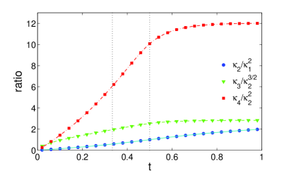
Here, $\kappa_{1}$ is the mean value, $\kappa_{2}$ the variance, while the skewness and kurtosis are given as $\kappa_{3}/\kappa_{2}^{3/2}$ and $\kappa_{4}/\kappa_{2}^{2}$, respectively. We note that the expression for the variance $\kappa_{2}$ reproduces the result by Qian et al. which was obtained for a discrete random walk [7]. In turn, the formulas for the third and fourth moments are derived for the first time.

Figure 2: (Color online) (Left) The reduced variance $\kappa_{2}/\kappa_{1}^{2}$, skewness $\kappa_{3}/\kappa_{2}^{3/2}$ and kurtosis $\kappa_{4}/\kappa_{2}^{2}$ of the TAMSD $\chi_{t}$ as functions of the lag time $t$. Symbols present the values obtained from an exact matrix formula for a discrete random walk (see Eq. (6) from [37], the sample length $N=1000$), while lines refer to the analytical formulas (13), (14), (15) for $t>1/2$ and (17), (18), (3.1.2) (or (20)) for $t<1/2$. (Right) The relative error between the analytical formulas and their counterparts for a discrete random walk. The vertical dotted lines stand at $t=1/3$ and $t=1/2$. All the formulas are accurate for the whole region (an increase of the relative error at small $t$ is related to intrinsic differences between discrete and continuous processes).

3.1.2 Case $t<1/2$.

For the case $1/3<t<1/2$ ($m=2$), the explicit formula for $\varphi_{t}(s)$ is provided in A.3. Taking the derivatives with respect to $s$, we obtain the first cumulant moments:

$$\kappa_{1} = t,$$ (16)

$$\kappa_{2} = \frac{1}{3}~{}\frac{t^{3}(4-5t)}{(1-t)^{2}},$$ (17)

$$\kappa_{3} = \frac{2}{15}~{}\frac{t^{5}(33-47t)}{(1-t)^{3}},$$ (18)

$$\kappa_{4} = \frac{2}{105}(1-t)^{-4}\biggl{[}30913t^{8}-86272t^{7}+102060t^{6}$$

$$-68040t^{5}+28350t^{4}-7560t^{3}+1260t^{2}-120t+5\biggr{]}.$$

As the explicit formula (10) for $\varphi_{t}(s)$ is too cumbersome for $t<1/3$, another representation (61) for the cumulant moments was deduced in B. In particular, we checked that Eqs. (17) and (18) for $\kappa_{2}$ and $\kappa_{3}$ are also valid for $t<1/3$. In turn, the formula for $\kappa_{4}$ for $t<1/3$ becomes

$$\kappa_{4}=\frac{8t^{7}}{105(1-t)^{4}}(302-473t)\qquad(t<1/3).$$ (20)

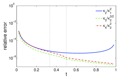
Figure 2 shows the reduced variance $\kappa_{2}/\kappa_{1}^{2}$, skewness $\kappa_{3}/\kappa_{2}^{3/2}$ and kurtosis $\kappa_{4}/\kappa_{2}^{2}$ of the TAMSD as functions of the lag time $t$. The values obtained from an exact matrix formula for a discrete random walk (see Eq. (6) from [37], the sample length $N=1000$), are compared to the analytical formulas (13), (14), (15) for $t>1/2$ and (17), (18), (3.1.2) (or (20)) for $t<1/2$. Notice an excellent agreement between the curves.

3.2 Small $z$ asymptotic behavior

3.2.1 Case $t>\frac{1}{2}$

In the limit of large $s$, Eq. (8) can be approximated as

$$\varphi_{t}(s)\approx\frac{2e^{-\sqrt{s(1-t)}}}{\sqrt{\sqrt{s(1-t)}~{}\frac{3t-1}{1-t}}}\qquad(s\gg 1).$$

Using the asymptotic relation for the inverse Laplace transform ${\mathcal{L}}^{-1}$,

$${\mathcal{L}}^{-1}[s^{\kappa}e^{-2\sqrt{as}}]\approx\frac{a^{\kappa+1/2}}{\sqrt{\pi}}z^{-2\kappa-3/2}e^{-a/z},$$ (21)

with $\kappa=-1/4$ and $a=(1-t)/4$, one derives the asymptotic behavior of the probability density $p_{t}(z)$ at small $z$:

$$p_{t}(z)\approx\frac{2}{\sqrt{2\pi\frac{3t-1}{1-t}}}~{}\frac{e^{-(1-t)/(4z)}}{z}\qquad(z\to 0).$$ (22)

In other words, the asymptotic decay of $\varphi_{t}(s)$ as $e^{-2\sqrt{as}}$ at large $s$ implies the sharp decay of $p_{t}(z)$ as $e^{-a/z}$ at small $z$. This is the first rigorous justification for using a GGD in Eq. (2) to approximate the probability density $p_{t}(z)$.

3.2.2 Case $t<\frac{1}{2}$

In this case, we have to analyze the asymptotic behavior of Eqs. (9) or (10). For large $s$, one can replace $\sinh(z)$ by $e^{z}/2$ (with exponentially small corrections) to get in both cases

$$\varphi_{t}(s)\approx\frac{\exp\left(-\sqrt{s}\frac{\eta(t)}{\sqrt{2(1-t)}}\right)}{\sqrt{I_{t}(g)}}\qquad(s\gg 1).$$ (23)

where the functions $\eta(t)$ and $I_{t}(g)$ are explicitly given in A. The asymptotic behavior of $\varphi_{t}(s)$ at large $s$ is mainly determined by the exponential term, while $I_{t}(g)$ turns out to be an algebraic correction. In C, we derive a representation of $I_{t}(g)$ in the form $I_{t}(g)=c_{0}+c_{1}g$, where $c_{0}$ and $c_{1}$ become independent of $g$ for large $g$ (or $s$). As a consequence, the asymptotic behavior of $\varphi_{t}(s)$ reads as

$$\varphi_{t}(s)\simeq\frac{\exp\left(-\sqrt{s}\frac{\eta(t)}{\sqrt{2(1-t)}}\right)}{\sqrt{c_{0}+\frac{c_{1}\sqrt{2}}{\sqrt{1-t}}\sqrt{s}}}\qquad(s\gg 1).$$

Neglecting $c_{0}$ and using again Eq. (21), one deduces the asymptotic behavior of $p_{t}(z)$:

$$p_{t}(z)\approx\frac{\sqrt{\eta(t)}}{\sqrt{2\pi c_{1}(t)}}~{}z^{-1}\exp\left(-\frac{\eta^{2}(t)}{8z(1-t)}\right)\qquad(z\to 0),$$ (24)

in which $c_{1}(t)$ is given by Eq. (65). Similar to the case $t>\frac{1}{2}$, the probability density sharply decays (as $e^{-a/z}$) when $z\to 0$.

3.3 Large $z$ asymptotic behavior

Since the inverse Laplace transform can be written as the Bromwich integral in the complex plane, the singularities of $\varphi_{t}(s)$ for $s\in{\mathbb{C}}$ play an important role. In particular, the singularity with the largest (negative) real part, which is called the abscissa of convergence of the Laplace transform, determines the asymptotic behavior of the probability density $p_{t}(z)$ at large $z$ [38].

For $t>\frac{1}{2}$, one can easily check that all singularities of $\varphi_{t}(s)$ are located on the negative real axis. In fact, taking $s=-\alpha^{2}/(1-t)$, one can rewrite Eq. (8) as

$$\varphi_{t}(s)=\frac{2}{\cos\alpha}\left(1-\beta^{-1}~{}\alpha\tan\alpha\right)^{-1/2},$$ (25)

where $\beta=(1-t)/(3t-1)$ is a positive parameter between $0$ and $1$ (given that $\frac{1}{2}\leq t\leq 1$). This function has two sets of singularities at points $\tilde{\alpha}_{k}$ and $\alpha_{k}$ which are solutions of the equations

$$\cos\tilde{\alpha}_{k}=0,\qquad\alpha_{k}\tan\alpha_{k}=\beta\qquad(k=1,2,3,...).$$

The smallest solution $\alpha_{1}$ of the second equation can be determined perturbatively in powers of $\beta$:

$$\alpha_{1}^{2}=\beta-\frac{1}{3}\beta^{2}+\frac{4}{45}\beta^{3}+O(\beta^{4}).$$

The related singularity is thus located at

$$s_{1}=-\frac{\alpha_{1}^{2}}{1-t}=-\left(\frac{1}{3t-1}-\frac{1-t}{3(3t-1)^{2}}+\frac{4(1-t)^{2}}{45(3t-1)^{3}}+O((1-t)^{3})\right).$$

Note that $\alpha_{1}$ varies from $0$ at $t=1$ to $0.8603...$ at $t=0.5$ so that $|s_{1}|$ varies from $0.5$ at $t=1$ to $1.4803$ at $t=0.5$. At the same time, the smallest solution $\tilde{\alpha}_{1}=\pi/2$ is independent of $t$ and is always larger than $\alpha_{1}$.

In close vicinity of $s_{1}$, one has

$$\varphi_{t}(s)\simeq\sqrt{\frac{2(\beta^{2}+\alpha_{1}^{2})}{(\beta+\beta^{2}+\alpha_{1}^{2})(3t-1)}}~{}(s-s_{1})^{-1/2}\qquad(s\approx s_{1}),$$

from which the inverse Laplace transform yields an asymptotic approximation

$$p_{t}(z)\simeq\sqrt{\frac{2(\beta^{2}+\alpha_{1}^{2})}{(\beta+\beta^{2}+\alpha_{1}^{2})(3t-1)}}~{}\frac{\exp(-z/b)}{\sqrt{\pi z}}\qquad(z\gg 1),$$ (26)

with $b=1/|s_{1}|=(1-t)/\alpha_{1}^{2}$.

The analysis can be extended to the case $t<\frac{1}{2}$. For instance, when $t=1/m$, one can substitute $s=-(1-t)\alpha^{2}/(2t)$ into Eq. (9) in order to locate the singularities of $\varphi_{t}(s)$ either as solutions $\tilde{\alpha}_{k}$ of $\sin(\tilde{\alpha}_{k}\sqrt{\lambda_{k}})=0$ (with $k=1,...,m-1$), or as solutions $\alpha_{k}$ of $\det(\mathbf{A})=0$. For a general situation $\frac{1}{m+1}<t<\frac{1}{m}$ for some $m=2,3,4,...$, the singularties of $\varphi_{t}(s)$ can be determined in a similar way. In both cases, the large $z$ asymptotic behavior is determined by the largest negative root $s_{1}$ (i.e., the root with the smallest absolute value $|s_{1}|$) of the equation $\det(\mathbf{A})=0$. Given the square root type of singularity in Eq. (10), the exponential asymptotic decay of $p_{t}(z)$ at large $z$ in the form similar to Eq. (26) is expected to be valid for any lag time $t$.

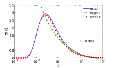
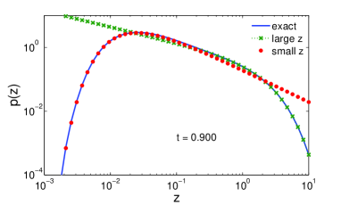
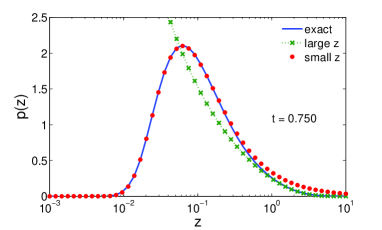
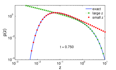
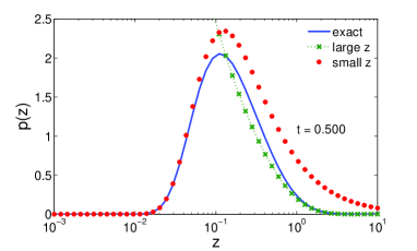
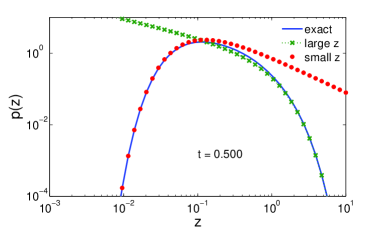
The accuracy of the asymptotic Eq. (22) for small $z$ and Eq. (26) for large $z$ is illustrated on Fig. 3. For all lag times, Eqs. (22),(24) correctly describe the asymptotic behavior of $p_{t}(z)$ at small $z$. Moreover, for larger $t$ (e.g., $t=0.9$ and $t=0.75$), Eq. (22) turns out to reproduce the whole shape of $p_{t}(z)$, except for large $z$. The deviations at large $z$ are expected because the exponential decay of $p_{t}(z)$ is not captured in the small $z$ asymptotic relation (22).

Figure 3: (Color online) The probability density $p_{t}(z)$ (solid line), its small $z$ asymptotic relation (22) (shown by circles), and large $z$ asymptotic relation (26) (shown by crosses), at lag times $t=0.9$, $t=0.75$ and $t=0.5$, in semilog (left) and loglog (right) scales.

3.4 Limiting case $t=1$

In the limit $t\to 1$, one gets $\varphi_{1}(s)=1/\sqrt{1+2s}$, from which

$$p_{1}(z)=\frac{e^{-z/2}}{\sqrt{2\pi z}}.$$ (27)

We retrieved therefore the limiting behavior of the discrete case for the lag time $n=N-1$ [7, 37]. Since the density $p_{1}(z)$ describes the distribution of a squared Gaussian variable $\chi_{1}=X^{2}(1)$, $\varphi_{1}(s)$ and then Eq. (27) could be directly obtained by integrating the Gaussian probability density $\frac{1}{\sqrt{2\pi}}e^{-x^{2}/2}$ for $X(1)$ with $e^{-sx^{2}}$.

The function $p_{1}(z)$ diverges at $z=0$ and monotonously decreases on the positive semi-axis $z>0$, in sharp contract to $p_{t}(z)$ (with $t<1$), which must have a maximum, as being equal to $0$ at $z=0$ and $z\to\infty$. In the limit $t\to 1$, the most probable value of $\chi_{t}$ (i.e., the position of the maximum) approaches $0$, while the mean value approaches $1$. This also illustrates the fact that $p_{1}(z)$ has the largest skewness among $p_{t}(z)$, as seen on Fig. 2.

3.5 Limiting case $t\to 0$

In the opposite limit of $t\to 0$ it is harder to get analytic behavior from theoretical results, as the limit describes the situation where the number of particles $m$ grows to infinity, which, combined with complicated boundary conditions for normal modes, makes a direct evaluation unfeasible. We provide here a few qualitative arguments, while a more rigorous analysis is reported in D. Since the mean and variance of $\chi_{t}$ vanish as $t\to 0$, it is convenient to rescale $\chi_{t}$ by $t$, in order to fix the mean value to $1$. For small $t$, the rescaled TAMSD can be approximated as

$$\tilde{\chi}_{t}\equiv\frac{\chi_{t}}{t}\simeq\frac{1}{m}\sum\limits_{k=1}^{m}\zeta_{k}^{2},$$

where $m=[1/t]$ and $\zeta_{k}$ are independent Gaussian displacements (standing for $X(t_{0}+t)-X(t_{0})$, with $t_{0}=kt$) with mean zero and variance $1$. The above sum is known to have a chi-squared (or Gamma) distribution with $m$ degrees of freedom [39], from which

$$\tilde{\varphi}_{t}(s)\simeq(1+2s/m)^{-m/2}\simeq(1+2st)^{-1/(2t)}.$$ (28)

In the limit $t\to 0$, we get $\tilde{\varphi}_{0}(s)=e^{-s}$ and $\tilde{p}_{0}(z)=\delta(z-1)$ as expected since $\chi_{t}/t$ concentrates around $1$ in this limit. Although the limiting results for $\tilde{\varphi}_{0}(s)$ and $\tilde{p}_{0}(z)$ are correct, an approximation (28) of $\tilde{\varphi}_{t}(s)$ for small $t$ by a Gamma distribution is not accurate.

3.6 Dimensional units

All the above results were obtained for $D=1/2$ and $T=1$, with $t$ being a dimensionless lag time between $0$ and $1$. Dimensional units can be easily incorporated by replacing $s$ by $2DTs$, $z$ by $z/(2DT)$ and $t$ by $t/T$ in the formulas for $\varphi_{t}(s)$ and $p_{t}(z)$. For instance, Eq. (8) reads for a given diffusion coefficient $D$ and sample duration $T$ as

$$\varphi_{t}(s)=\frac{2e^{-\sqrt{2Ds(T-t)}}}{1+e^{-2\sqrt{2Ds(T-t)}}}~{}\left(1+\sqrt{2Ds(T-t)}~{}\frac{3t-T}{T-t}~{}\frac{1-e^{-2\sqrt{2Ds(T-t)}}}{1+e^{-2\sqrt{2Ds(T-t)}}}\right)^{-1/2}.$$

In the formulas for the cumulant moments, one has to replace $t$ by $t/T$ and multiply the right-hand side by $(2DT)^{n}$, with $n$ being the order of the moment.

3.7 Discrete versus continuous cases

As we discussed in Introduction, the TAMSD is commonly employed for inferring the diffusion coefficient from an individual random trajectory of a diffusing tracer. For this purpose, one records positions of a tracer at successive times, with a fixed time step $\tau$. An individual trajectory of the tracer is therefore discretized, and the TAMSD becomes

$$\chi_{n,N}=\frac{1}{N-n}\sum\limits_{k=1}^{N-n}(x_{k+n}-x_{k})^{2},$$ (29)

where $x_{k}=X(k\tau)$ is the position of the tracer at time $k\tau$, $n=t/\tau$ is the discrete lag time, and $N=T/\tau$ is the number of points in the sample. In the limit $\tau\to 0$, the discrete TAMSD is expected to converge to the continuous one defined by Eq. (1). The probability distribution of the TAMSD for a discrete Gaussian process was investigated in [37]. For a given covariance matrix $\mathbf{C}$ (and zero mean), one can use the classical matrix representation

$$\varphi_{n,N}(s)\equiv\langle\exp(-s\chi_{n,N})\rangle=\frac{1}{\sqrt{\det(\mathbf{I}+s\mathbf{M}\mathbf{C})}},$$ (30)

where the matrix $\mathbf{M}$ represents the discrete quadratic form in Eq. (29). When the sample length $N$ is smaller than few thousands, the Schur decomposition of the matrix $\mathbf{M}\mathbf{C}$ allows one to rapidly compute the Laplace transform $\varphi_{n,N}(s)$ or the characteristic function $\phi_{n,N}(k)\equiv\varphi_{n,N}(-ik)$, from which the probability density $p(z)$ can be reconstructed through the inverse Fourier transform [37].

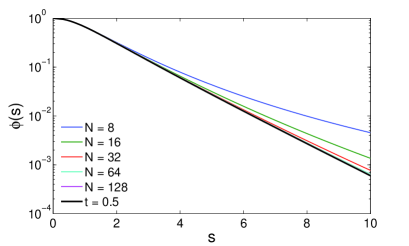
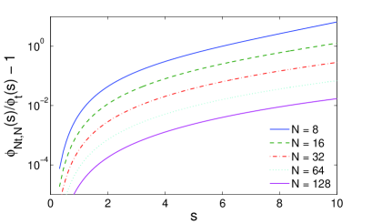
Although Eq. (30) provides an exact solution for $\varphi_{n,N}(s)$ and an efficient numerical way for computing $p(z)$ for moderate $N$, the dependence on the parameters (e.g., the lag time) remains elusive. In contrast, Eq. (8) for Brownian motion is explicit and allows one to derive the asymptotic behavior and the dependence on the lag time. Since $\chi_{n,N}$ approaches $\chi_{t,T}$ in the limit $\tau\to 0$, Eq. (8) is expected to be an accurate approximation to $\varphi_{n,N}(s)$ for large enough $N$. This point is illustrated on Fig. 4, in which $\varphi_{t}(s)$ for $t=0.5$ is compared to $\varphi_{N/2,N}(s)$, for different sample lengths $N$. The curves for $N=8,16,32$ exhibit deviations at large $s$, while the curves for larger $N=64,128$ are barely distinguishable from $\varphi_{t}(s)$ at the present range of $s$ values. As a consequence, one can use the explicit formula (8) for discrete samples with $N\gtrsim 50$. At the same time, the functions $\varphi_{n,N}(s)$ and $\varphi_{t}(s)$ will always be different for large enough $s$. In fact, for a fixed $N$, $\varphi_{n,N}(s)$ exhibits a power law asymptotic decay (as $\det(\mathbf{I}+s\mathbf{M}\mathbf{C})$ is a polynomial in $s$), while $\varphi_{t}(s)$ decays exponentially fast. However, the distinction between these behaviors may appear for so large $s$, for which both functions become already extremely small so that a distinction would be irrelevant for practical applications. In summary, Eq. (8) and its extensions for $t<1/2$ can in practice be used for studying the TAMSD of discretely sampled positions of a freely diffusing particle.

Figure 4: (Color online) (Left) Comparison between $\varphi_{t}(s)$ for Brownian motion (with $t=0.5$) from Eq. (8) (thick black line) and $\varphi_{Nt,N}(s)$ for discrete random walks with different sample length $N=8,16,32,64,128$, with $n=tN$. The curves for $N=64,128$ are barely distinguishable from the theoretical one. (Right) The relative error between $\varphi_{t}(s)$ and $\varphi_{Nt,N}(s)$. As expected, the relative error increases with $s$ and it is larger for smaller $N$.

3.8 Relation to generalized Gamma distribution

As shown numerically in [37], the probability density $p_{t}(z)$ for a discrete random walk can be accurately approximated by a generalized Gamma distribution (GGD) from Eq. (2). Its Laplace transform reads as

$$\varphi(s)=(1+sb)^{-\nu/2}\frac{K_{\nu}(2\sqrt{a(1+sb)/b})}{K_{\nu}(2\sqrt{a/b})}.$$ (31)

On one hand, its comparison to Eqs. (8), (9), (10) immediately shows that a GGD is not an exact distribution for $\chi_{t}$ (except for the trivial case $t=1$). On the other hand, we have seen earlier that the GGD correctly reproduces the asymptotic behavior at small and large $z$, and it turns out to be a remarkably accurate approximation of $p_{t}(z)$ (see Fig. 6). Moreover, a simple form of Eq. (2) is particularly attractive for practical purposes (e.g., inferring statistics of diffusion coefficients by maximum likelihood methods, estimating the confidence intervals, etc.). For practical uses of this approximation, it is important to relate the parameters $a$, $b$ and $\nu$ to the lag time $t$.

In E, we derive the asymptotic relations for the parameters $a$, $b$ and $\nu$ in the limit $t\to 0$ by matching the first three moments:

$$c = x\nu\simeq\frac{3\sqrt{1159}}{160}~{}t^{-1}+c_{0}\approx 0.638~{}t^{-1}-0.537,$$ (32)

$$\nu = \frac{1}{\varepsilon}\simeq\frac{63}{160}~{}t^{-1}+\nu_{0}\approx 0.394~{}t^{-1}-0.714,$$ (33)

$$a = \frac{x}{1+\sqrt{1+x^{2}}}~{}\frac{tc}{2}\simeq\frac{57}{320}+a_{0}t\approx 0.178-0.105t,$$ (34)

$$b = \frac{4a}{c^{2}}\simeq\frac{320}{183}~{}t^{2}+b_{3}t^{3}\approx 1.749~{}t^{2}+2.3t^{3},$$ (35)

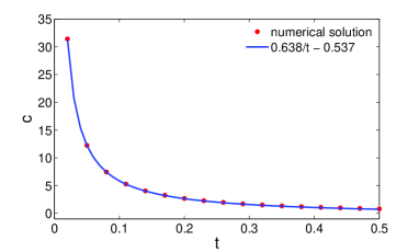
where $c=2\sqrt{a/b}$ and $x=\frac{\sqrt{1159}}{21}\approx 1.6211$. Here, the leading terms were derived analytically, while the values of the next-order corrections $\nu_{0}$, $c_{0}$, $a_{0}$ and $b_{0}$ were obtained by fitting the numerical curves of these quantities. Although they could in principle be found from the higher-order terms, such analysis goes beyond the scope of the paper. The asymptotic relations (32), (33), (34), (35) turn out to be accurate for the whole range of $t<\frac{1}{2}$, as shown on Fig. 5.

Figure 5: (Color online) The parameters $a$, $b$ and $\nu$ (and $c=2\sqrt{a/b}$) of the GGD as functions of the lag time $t$. Full circles are obtained by a numerical resolution of Eqs. (71), (72) and solid lines represent the short-time asymptotic formulas (32), (33), (34), (35) for $t<\frac{1}{2}$.

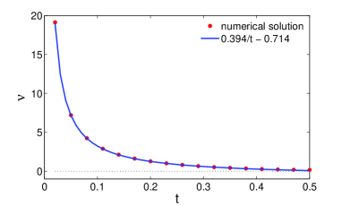
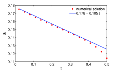
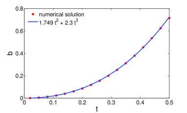
We check the accuracy of the GGD with the parameters $a$, $b$ and $\nu$ from the short-time asymptotic formulas (33), (34), (35) by comparing this approximation to the probability density obtained numerically for a discrete random walk (Sect. 3.7). The latter is referred here as “exact” solution, although it was obtained by a numerical computation of the inverse Fourier transform of the exact characteristic function from Eq. (30), as explained in detail in [37]. In order to plot several curves onto the same figure, the TAMSD was rescaled by $t$ to set the mean value to $1$ for all lag times $t$. Figure 6(left) shows an excellent agreement between exact solutions and approximations by the GGD, for several lag times $t$ from $0$ to $\frac{1}{2}$.

Figure 6: (Color online) The probability density $p_{t}(z)$ of the TAMSD rescaled by $t$ for several lag times $t$, in normal, semilog and loglog scales. Lines show exact solutions for a discrete random walk, while circles represent approximations by GGDs. For $t\leq\frac{1}{2}$ (left panel), the parameters $a$, $b$ and $\nu$ are obtained from the asymptotic formulas (33), (34), (35). Even for the limiting value $t=\frac{1}{2}$, the approximation remains accurate. For $t>\frac{1}{2}$ (right panel), the parameters $a$, $b$ and $\nu$ are extracted from the best fit of $p_{t}(z)$ by a GGD.

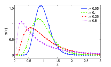
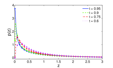
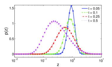
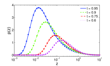
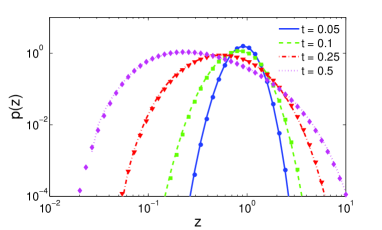
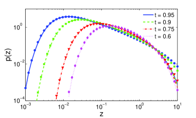
For larger lag times, the probability density $p_{t}(z)$ becomes more and more skewed, with the maximum of $p_{t}(z)$ getting much smaller than the mean value. As a consequence, positive-order moments are determined by the values of $p_{t}(z)$ far from the maximum. Given the objective to approximate the function $p_{t}(z)$ around the maximum, one cannot therefore rely on matching positive-order moments, as done in E. One needs therefore to identify other characteristics of the true and approximate distributions to be matched. One can see that even with the exact solution at hand, the analysis is intricate.

At the same time, GGD remains an accurate approximation of the probability density $p_{t}(z)$ even for $t>\frac{1}{2}$, as illustrated on Fig. 6 (right panel). On the right panel, the parameters $a$, $b$ and $\nu$ were obtained by fitting the exact density $p_{t}(z)$ (obtained numerically) to a GGD. As a perspective, one may attempt to derive analytical asymptotic relations for these parameters for $t>\frac{1}{2}$. Note also that, for $t>\frac{1}{2}$, the small $z$ asymptotic formula (22) is also an accurate approximation of $p_{t}(z)$, as discussed in Sect. 3.2.

3.9 Two-dimensional and higher-dimensional case

The above analysis was focused on a one-dimensional Brownian motion. In turn, many SPT techniques allow one to record the displacements of a tracer in two or three dimensions. Under the assumption of isotropic motion, one often considers the combined time-averaged MSD

$$\chi^{(d)}_{t,T}=\frac{1}{T-t}\int\limits_{0}^{T-t}dt_{0}\sum\limits_{i=1}^{d}\bigl{(}X_{i}(t_{0}+t)-X_{i}(t_{0})\bigr{)}^{2},$$ (36)

where $X_{i}(t)$ is the tracer’s position at time $t$ along the $i$th coordinate. For $d$-dimensional Brownian motion, each process $X_{i}(t)$ is a one-dimensional Brownian motion independent from the others so that the Laplace transform $\varphi_{t}^{(d)}(s)$ for the random variable $\chi^{(d)}_{t,T}$ is simply $[\varphi_{t}(s)]^{d}$. One can then easily extend the above 1D results to higher-dimensional cases. In particular, the probability density $p(z)$ would exhibit similar asymptotic behavior at small and large $z$, with deviations coming from power law corrections.

Conclusion

We have studied the statistical properties of the time-averaged mean-square displacements of Brownian motion. Using the standard tools of functional integrals, the original problem was mapped onto an exactly solvable model of coupled harmonic oscillators. When the lag time $t$ was larger than a half of the trajectory length $T$ ($t>T/2$), a simple closed formula (8) for the Laplace transform $\varphi_{t}(s)$ of the probability density $p_{t}(z)$ was derived. In the opposite case $t<T/2$, the analysis was quite similar, although the resulting exact formulas were less explicit. This reflects the many-body character of the original problem. In the special case $t=1/m$ with $m=2,3,4,...$, one dealt with a chain of coupled harmonic oscillators and derived Eq. (9) for $\varphi_{t}(s)$. The general situation corresponded to two chains of coupled harmonic oscillators, for which Eq. (10) for $\varphi_{t}(s)$ was deduced. From these formulas, the probability density $p_{t}(z)$ can be formally reconstructed either through the inverse Laplace transform of $\varphi_{t}(s)$, or through the inverse Fourier transform of the characteristic function $\phi_{t}(k)\equiv\varphi_{t}(-ik)$ (the second option being more convenient for numerical implementation). To our knowledge, the probability distribution of the TAMSD of Brownian motion was derived for the first time.

From the exact formulas for $\varphi_{t}(s)$, we deduced the first four cumulant moments of the TAMSD. While the first and second moments (mean and variance) were reported earlier, the third and fourth moments (related to skewness and kurtosis of the distribution) have been obtained for the first time. We also analyzed the asymptotic behavior of the probability density $p_{t}(z)$ at small and large arguments. In particular, we have shown the sharp decay of $p_{t}(z)$ as $e^{-a/z}$ at small $z$. This behavior justified the use of a generalized Gamma distribution as an approximation for $p_{t}(z)$ suggested in [37]. The fact that the GGD correctly reproduces the asymptotic behavior of the probability density at both small and large $z$ explained a remarkable accuracy of this approximation, illustrated by Fig. 6. Finally, we expressed the parameters $a$, $b$ and $\nu$ of a GGD as functions of the lag time $t$ by matching the first moments of the true and approximate distributions. The resulting asymptotic relations were shown to be accurate for $t<T/2$ so that one could easily construct an accurate approximation for the probability density $p_{t}(z)$ of the TAMSD for a given lag time. For larger $t$, the distribution was too skewed so that the first moments did not really control the shape of $p_{t}(z)$ around the maximum. In that case, one had to resort to a simple approximation of $p_{t}(z)$ provided by the asymptotic form (22) (i.e., by a GGD with $a=(1-t)/4$, $b=0$ and $\nu=0.5$). However, as illustrated on Fig. 6, better approximations by a GGD could be constructed. Their explicit derivation requires further analysis.

From a practical point of view, an accurate approximation of the probability density $p_{t}(z)$ by a simple function (such as a generalized Gamma distribution) opens several interesting perspectives for a more reliable analysis of random trajectories of diffusing tracers acquired in single-particle tracking experiments. In particular, one can develop efficient inferring schemes through maximum likelihood estimation, or accurately quantify the confidence intervals of measured diffusion coefficients. While the present work was focused on Brownian motion, future investigations may challenge the statistical properties of the TAMSD for more sophisticated processes (e.g., restricted diffusion, fractional Brownian motion or generalized Langevin equation with memory) which are known to be representative models for diffusive dynamics in viscoelastic media (e.g., living cells) or for time series in finance.

Appendix A Computation for $t<\frac{1}{2}$

The computation for the case $t<\frac{1}{2}$ is a straightforward generalization of the calculus from Sect. 2.1. For convenience, we consider separately the special case $t=\frac{1}{m}$ in A.1 and the generic case $\frac{1}{m+1}<t<\frac{1}{m}$ in A.2.

A.1 Special cases $t=\frac{1}{m}$

For $t=\frac{1}{m}$ with $m=2,3,4,...$, the whole time interval $[0,1]$ is covered by $m$ equal subintervals so that the trajectory can be mapped onto a chain of $m$ coupled harmonic oscillators as illustrated on Fig. 1b. We define oscillators $Y_{k}$ as

$$Y_{k}(u)\equiv X(kt+u)\qquad u\in(0,t),~{}~{}(k=0...m-1),$$

so that the non-local part of the action in Eq. (5) becomes:

$$\int\limits_{0}^{1-t}du(X(u+t)-X(u))^{2}=\sum\limits_{k=0}^{m-2}\int\limits_{kt}^{(k+1)t}du(X(u+t)-X(u))^{2}=\sum\limits_{k=0}^{m-2}\int\limits_{0}^{t}du(Y_{k+1}(u)-Y_{k}(u))^{2},$$

from which the Laplace transform reads as

$$\varphi_{t}(s)=\int\limits_{{\mathbb{R}}^{m}}dy_{1}...dy_{m}\prod_{k=0}^{m-1}\int_{Y_{k}(0)=y_{k}}^{Y_{k}(t)=y_{k+1}}\mathcal{D}Y_{k}\,\exp\left[-\frac{1}{2}\int_{0}^{t}(\partial_{u}Y_{k})^{2}-\frac{g^{2}}{2}\int_{0}^{t}(Y_{k+1}-Y_{k})^{2}\right],$$

with the starting point $y_{0}=0$ (and $y_{m}=x_{1}$). The non-locality is therefore eliminated at the expense of many-body character of the resulting problem. To advance further we need to diagonalize the chain of coupled oscillators with open boundary conditions:

$$\Sigma=\sum_{k=0}^{m-1}\int_{0}^{t}(\partial_{u}Y_{k})^{2}+g^{2}\sum_{k=0}^{m-2}\int_{0}^{t}(Y_{k+1}-Y_{k})^{2}=\sum_{k=0}^{m-1}\int_{0}^{t}\left[(\partial_{u}Y_{k})^{2}+g^{2}\sum\limits_{l=0}^{m-1}Y_{k}L_{kl}Y_{l}\right],$$

where the matrix $\mathbf{L}$ is a discrete Laplacian of size $m\times m$ with von Neumann boundary conditions:

$$\mathbf{L}=\left(\begin{array}[]{c c c c c c c}1&-1&0&0&\cdots&0&0\\ -1&2&-1&0&\cdots&0&0\\ 0&-1&2&-1&\cdots&0&0\\ 0&0&-1&2&\cdots&0&0\\ 0&0&0&-1&\cdots&0&0\\ \cdots&\cdots&\cdots&\cdots&\cdots&\cdots&\cdots\\ 0&0&0&0&\cdots&-1&1\\ \end{array}\right).$$

The normal modes which diagonalize $\Sigma$ are defined as

$$A_{k}=\sum_{l=0}^{m-1}\Psi_{kl}Y_{l}\qquad(k=0,\dots,m-1),$$

where $\mathbf{\Psi}$ is an orthogonal matrix with columns formed by eigenvectors of $\mathbf{L}$: $\mathbf{L}\cdot\mathbf{\Psi}=\mathbf{\Psi}\cdot\mathbf{\Lambda}$. It is straightfoward to compute the eigenvalues and eigenvectors of this matrix:

$$\Lambda_{kl}=\delta_{kl}\lambda_{k},\qquad\lambda_{k}=2\left(1-\cos\frac{\pi k}{m}\right)\qquad(k=0...m-1),$$ (37)

$$\Psi_{kl}=\frac{\sin\frac{\pi k(l+1)}{m}-\sin\frac{\pi kl}{m}}{\sqrt{m(1-\cos\frac{\pi k}{m})}}\qquad(k=1...m-1,~{}l=0...m-1),$$ (38)

$$\Psi_{0l}=\frac{1}{\sqrt{m}}\qquad(l=0...m-1).$$

We obtain the diagonalized form as

$$\Sigma=\sum_{k=0}^{m-1}\int_{0}^{t}\left[(\partial_{u}A_{k})^{2}+g^{2}\lambda_{k}A_{k}^{2}\right]$$ (39)

(note that for $k=0$ the second term vanishes as $\lambda_{0}=0$), with the boundary conditions for $A_{k}$ translated from the boundary conditions for $Y_{k}$ as

$$a_{k0} = A_{k}(0)=\sum_{l=0}^{m-1}\Psi_{kl}Y_{l}(0)=\sum_{l=1}^{m-1}\Psi_{kl}y_{l}\qquad(k=0..m-1),$$

$$a_{kt} = A_{k}(t)=\sum_{l=0}^{m-1}\Psi_{kl}Y_{l}(t)=\sum_{l=0}^{m-1}\Psi_{kl}y_{l+1}\qquad(k=0..m-1).$$ (40)

These linear relations convert the original coordinates $y_{1},\dots,y_{m}$ into new variables $a_{k0}$ and $a_{kt}$. In the first relation, the sum runs from $l=1$ as $y_{0}=0$ and the columns of the matrix $\mathbf{\Psi}$ are shifted to the left, the last column being filled with zeros (as there is no dependence on $y_{m}$). This shift can be represented by a shift matrix $\mathbf{S}$ (of size $m\times m$) as $\mathbf{\Psi}\cdot\mathbf{S}$:

$$\mathbf{S}=\left(\begin{array}[]{c c c c c}0&0&...&0&0\\ 1&0&...&0&0\\ 0&1&...&0&0\\ ...&...&...&...&...\\ 0&0&...&1&0\\ \end{array}\right).$$

Using the shift matrix, we can write

$$a_{k0}=\sum\limits_{l=0}^{m-1}[\mathbf{\Psi}\cdot\mathbf{S}]_{kl}y_{l+1}\qquad(k=0...m-1).$$ (41)

Once we have the diagonalized form (39), the Feynman-Kac formula is applicable and the Laplace transform $\varphi_{t}(s)$ is again given as a product of $m-1$ propagators of harmonic oscillators and one propagator of a free particle (corresponding to $\lambda_{0}=0$):

$$\varphi_{t}(s)=\int\limits_{{\mathbb{R}}^{m}}dy_{1}\cdots dy_{m}\,G_{0}(a_{0t},t|a_{00},0)\,\prod\limits_{k=1}^{m-1}G_{g\sqrt{\lambda_{k}}}(a_{kt},t|a_{k0},0).$$

We plug in the propagators as given by Eq. (6) and find the following expression:

$$\varphi_{t}(s) = \int\limits_{{\mathbb{R}}^{m}}dy_{1}\cdots dy_{m}\,\frac{1}{\sqrt{2\pi t}}\,\exp\left(-\frac{(a_{0t}-a_{00})^{2}}{2t}\right)$$

$$\times \prod\limits_{k=1}^{m-1}\frac{(g\sqrt{\lambda_{k}})^{1/2}e^{-tg\sqrt{\lambda_{k}}}}{\sqrt{\pi(1-q_{k}^{2})}}\exp\left(-\frac{\alpha_{k}g\sqrt{\lambda_{k}}}{4}(a_{kt}+a_{k0})^{2}-\frac{g\sqrt{\lambda_{k}}}{4\alpha_{k}}(a_{kt}-a_{k0})^{2}\right),$$

where

$$q_{k}=e^{-tg\sqrt{\lambda_{k}}},\qquad\alpha_{k}=\frac{1-q_{k}}{1+q_{k}}.$$ (43)

The formula for $\varphi_{t}(s)$ can be rewritten as

$$\varphi_{t}(s)=\frac{\exp\left(-\frac{1}{2}g\eta(t)\right)}{\prod\limits_{k=1}^{m-1}(1+q_{k})}~{}\frac{1}{\sqrt{I_{t}(g)}},$$ (44)

in which

$$\eta(t)=t\sum\limits_{k=1}^{m-1}\sqrt{\lambda_{k}}=t\biggl{(}{\rm ctan}\bigl{(}\frac{\pi}{4m}\bigr{)}-1\biggr{)},$$ (45)

$$\frac{1}{\sqrt{I_{t}(g)}}=\frac{1}{\sqrt{2\pi t}}~{}\frac{g^{(m-1)/2}}{\pi^{(m-1)/2}}\left(\prod\limits_{k=1}^{m-1}\frac{\sqrt{\lambda_{k}}}{\alpha_{k}}\right)^{1/2}\int\limits_{{\mathbb{R}}^{m}}d{\bf y}\exp\left(-\frac{1}{2}({\bf y}^{T}\cdot\mathbf{A}\cdot{\bf y})\right),$$ (46)

where ${\bf y}=(y_{1},...,y_{m})^{T}$, and $\mathbf{A}=\mathbf{V}^{T}\cdot\mathbf{U}\mathbf{V}$ is the matrix of size $m\times m$ which combines both the structure of the quadratic form in Eq. (A.1) and the linear relations (40), (41), represented respectively by matrices $\mathbf{U}$ and $\mathbf{V}$ of sizes $2m\times 2m$ and $2m\times m$:

$$\mathbf{U}=\left(\begin{array}[]{c | c}\mathbf{U}^{+}&\mathbf{U}^{-}\\ \hline\cr\mathbf{U}^{-}&\mathbf{U}^{+}\\ \end{array}\right),\qquad\mathbf{V}=\left(\begin{array}[]{c}\mathbf{\Psi}\cdot\mathbf{S}\\ \hline\cr\mathbf{\Psi}\\ \end{array}\right),$$ (47)

where $U^{\pm}$ are diagonal matrices of size $m\times m$ with the elements

$$u_{k}^{+} = \frac{1}{2}g\sqrt{\lambda_{k}}(\alpha_{k}+1/\alpha_{k})=\frac{g\sqrt{\lambda_{k}}}{\tanh(gt\sqrt{\lambda_{k}})}\quad(k=1...m-1),\qquad u_{0}^{+}=\frac{1}{t},$$

$$u_{k}^{-} = \frac{1}{2}g\sqrt{\lambda_{k}}(\alpha_{k}-1/\alpha_{k})=\frac{-g\sqrt{\lambda_{k}}}{\sinh(gt\sqrt{\lambda_{k}})}\quad(k=1...m-1),\qquad u_{0}^{-}=\frac{-1}{t}.$$

The elements $u_{0}^{\pm}$ can be seen as the limit of the generic formulas with $\lambda_{0}\to 0$. Performing the matrix multiplication yields

$$\mathbf{A}=\mathbf{V}^{T}\mathbf{U}\mathbf{V}=\mathbf{\Psi}^{T}\mathbf{U}^{+}\mathbf{\Psi}+\mathbf{S}^{T}\mathbf{\Psi}^{T}\mathbf{U}^{-}\mathbf{\Psi}+\mathbf{\Psi}^{T}\mathbf{U}^{-}\mathbf{\Psi}\mathbf{S}+\mathbf{S}^{T}\mathbf{\Psi}^{T}\mathbf{U}^{+}\mathbf{\Psi}\mathbf{S}.$$ (48)

The diagonal matrices $U^{\pm}$ contain the eigenvalues $\lambda_{k}$ of the original matrix $\mathbf{L}$ and $\mathbf{\Psi}$ is formed by its eigenvectors, implying a simple matrix representation for $\mathbf{A}$:

$$\mathbf{A}=\frac{g\sqrt{\mathbf{L}}}{\tanh(gt\sqrt{\mathbf{L}})}-\mathbf{S}^{T}\frac{g\sqrt{\mathbf{L}}}{\sinh(gt\sqrt{\mathbf{L}})}-\frac{g\sqrt{\mathbf{L}}}{\sinh(gt\sqrt{\mathbf{L}})}\mathbf{S}+\mathbf{S}^{T}\frac{g\sqrt{\mathbf{L}}}{\tanh(gt\sqrt{\mathbf{L}})}\mathbf{S}.$$ (49)

This expression is convenient for a theoretical analysis, while the original representation (48) is better suited for rapid numerical construction of $\mathbf{A}$.

The computation of the Gaussian integral in Eq. (46) yields

$$\frac{1}{\sqrt{I_{t}(g)}}=\frac{(2g)^{(m-1)/2}}{\sqrt{t}~{}\sqrt{\det(\mathbf{A})}}\left(\prod\limits_{k=1}^{m-1}\frac{\sqrt{\lambda_{k}}}{\alpha_{k}}\right)^{1/2}.$$ (50)

This relation, together with Eq. (44), completes the computation of $\varphi_{t}(s)$ for special cases $t=1/m$ (with $m=2,3,4,...$) and provides a solution to the problem. This solution can alternatively be written in the form (9).

A.2 Generic situation

For the generic case $\frac{1}{1+m}<t<\frac{1}{m}$ (for some $m=2,3,4,...$), the interval $[0,1]$ is covered by $m$ subintervals of duration $t$, plus a smaller interval $[mt,1]$ of duration $\delta=1-mt<t$. In order to split the interval $[0,1]$ regularly, one divides each subinterval in two parts, of durations $\delta$ and $t-\delta$, respectively:

$$[0,1]=[0,\delta]\cup[\delta,t]\cup\cdots\cup[t_{m-1},t_{m-1}+\delta]\cup[t_{m-1}+\delta,t_{m}]\cup[t_{m},1],$$

where $t_{k}=kt$. This covering maps the whole trajectory onto two interacting chains of $m+1$ and $m$ harmonic oscillators as illustrated on Fig. 1c:

$$Y_{k}(u) = X(t_{k}+u)\quad u\in[0,\delta],\quad(k=0\ldots m),$$

$$Z_{k}(u) = X(t_{k}+u)\quad u\in[\delta,t],\quad(k=0\ldots m-1).$$

Here $m=[1/t]$, the integer part of $1/t$. One gets therefore

$$\varphi_{t}(s)=\int\limits_{{\mathbb{R}}^{2m+1}}dy_{1}...dy_{m}dz_{0}...dz_{m}\prod_{k=0}^{m-1}\int_{Y_{k}(0)=y_{k}}^{Y_{k}(\delta)=z_{k}}\mathcal{D}Y_{k}\,\exp\left[-\frac{1}{2}\int_{0}^{\delta}(\partial_{u}Y_{k})^{2}-\frac{g^{2}}{2}\int_{0}^{\delta}(Y_{k+1}-Y_{k})^{2}\right]$$

$$\times\left\{\prod_{k=0}^{m-2}\int_{Z_{k}(0)=z_{k}}^{Z_{k}(t-\delta)=y_{k+1}}\mathcal{D}Z_{k}\,\exp\left[-\frac{1}{2}\int_{\delta}^{t}(\partial_{u}Z_{k})^{2}-\frac{g^{2}}{2}\int_{\delta}^{t}(Z_{k+1}-Z_{k})^{2}\right]\right\}$$

$$\times\int_{Y_{m}(0)=y_{m}}^{Y_{m}(\delta)=z_{m}}\mathcal{D}Y_{m}\,\exp\left[-\frac{1}{2}\int_{0}^{\delta}(\partial_{u}Y_{m})^{2}\right]\int_{Z_{m-1}(\delta)=z_{m-1}}^{Z_{m-1}(t)=y_{m}}\mathcal{D}Z_{m-1}\,\exp\left[-\frac{1}{2}\int_{\delta}^{t}(\partial_{u}Z_{m-1})^{2}\right].$$

(with $y_{0}=0$). There is no direct interaction between the two chains, but the boundary conditions for the chains are mixed since $Y_{k}(\delta)=Z_{k}(0)$ and $Z_{k}(t-\delta)=Y_{k+1}(0)$ to ensure the continuity of the original Brownian trajectory. Introducing normal modes:

$$A_{k}=\sum_{l=0}^{m}\tilde{\Psi}_{kl}Y_{l},\hskip 28.45274ptB_{k}=\sum_{l=0}^{m-1}\Psi_{kl}Z_{l},$$

this problem transforms into a set of uncoupled oscillators. The $\mathbf{\tilde{\Psi}}$ is an orthogonal matrix formed by the eigenvectors of the discrete Laplacian $\mathbf{L}$ of size $(m+1)\times(m+1)$ (tilde sign refers to quantities related to the matrix $\mathbf{L}$ of size $(m+1)\times(m+1)$, in order to distinguish them from similar quantities corresponding to $\mathbf{L}$ of size $m\times m$). The boundary conditions read for each $k=0\dots m$

$$a_{k0} = \sum_{k=1}^{m}\tilde{\Psi}_{kl}y_{l},\qquad a_{k\delta}=\sum_{l=0}^{m}\tilde{\Psi}_{kl}z_{l},$$ (51)

$$b_{k\delta} = \sum_{l=0}^{m-1}\Psi_{kl}z_{l},\qquad b_{kt}=\sum_{l=1}^{m}\Psi_{k,l-1}y_{l}.$$ (52)

We obtain then

$$\varphi_{t}(s)=\int\limits_{{\mathbb{R}}^{2m+1}}dy_{1}...dy_{m}dz_{0}...dz_{m}\left\{\prod\limits_{k=0}^{m}G_{g\sqrt{\tilde{\lambda}_{k}}}(a_{k\delta},\delta|a_{k0},0)\right\}\left\{\prod\limits_{k=0}^{m-1}G_{g\sqrt{\lambda_{k}}}(b_{kt},t|b_{k\delta},\delta)\right\}.$$

Note that two factors with $k=0$ correspond to free diffusion propagators (as $\lambda_{0}=\tilde{\lambda}_{0}=0$). Substituting Eq. (6) for the propagators, one gets Gaussian integrals:

$$\varphi_{t}(s) = \int\limits_{{\mathbb{R}}^{2m+1}}dy_{1}...dy_{m}dz_{0}...dz_{m}\frac{1}{2\pi\sqrt{\delta(t-\delta)}}\exp\left(-\frac{(a_{0\delta}-a_{00})^{2}}{2\delta}-\frac{(b_{0t}-b_{0\delta})^{2}}{2(t-\delta)}\right)$$

$$\times \prod\limits_{k=1}^{m}\frac{(g\sqrt{\tilde{\lambda}_{k}})^{1/2}e^{-\delta g\sqrt{\tilde{\lambda}_{k}}/2}}{\sqrt{\pi(1-\tilde{q}_{k}^{2})}}\exp\left(-\frac{\tilde{\alpha}_{k}g\sqrt{\tilde{\lambda}_{k}}}{4}(a_{k\delta}+a_{k0})^{2}-\frac{g\sqrt{\tilde{\lambda}_{k}}}{4\tilde{\alpha}_{k}}(a_{k\delta}-a_{k0})^{2}\right)$$

$$\times \prod\limits_{k=1}^{m-1}\frac{(g\sqrt{\lambda_{k}})^{1/2}e^{-(t-\delta)g\sqrt{\lambda_{k}}/2}}{\sqrt{\pi(1-q_{k}^{2})}}\exp\left(-\frac{\alpha_{k}g\sqrt{\lambda_{k}}}{4}(b_{kt}+b_{k\delta})^{2}-\frac{g\sqrt{\lambda_{k}}}{4\alpha_{k}}(b_{kt}-b_{k\delta})^{2}\right).$$

The argument of the exponential function can be represented as a quadratic form $\frac{1}{2}({\bf a}^{T}\mathbf{U}{\bf a})$:

$$\left(\begin{array}[]{c}a_{00}\\ ...\\ a_{m0}\\ b_{0t}\\ ...\\ b_{m-1,t}\\ a_{0\delta}\\ ...\\ a_{m\delta}\\ b_{0\delta}\\ ...\\ b_{m-1,\delta}\\ \end{array}\right)^{T}\left(\begin{array}[]{c c c c c c c c c c c c}\tilde{u}_{0}^{+}&...&0&0&...&0&\tilde{u}_{0}^{-}&...&0&0&...&0\\ ...&...&...&...&...&...&...&...&...&...&...&...\\ 0&...&\tilde{u}_{m}^{+}&0&...&0&0&...&\tilde{u}_{m}^{-}&0&...&0\\ 0&...&0&u_{0}^{+}&...&0&0&...&0&u_{0}^{-}&...&0\\ ...&...&...&...&...&...&...&...&...&...&...&...\\ 0&...&0&0&...&u_{m-1}^{+}&0&...&0&0&...&u_{m-1}^{-}\\ \tilde{u}_{0}^{-}&...&0&0&...&0&\tilde{u}_{0}^{+}&...&0&0&...&0\\ ...&...&...&...&...&...&...&...&...&...&...&...\\ 0&...&\tilde{u}_{m}^{-}&0&...&0&0&...&\tilde{u}_{m}^{+}&0&...&0\\ 0&...&0&u_{0}^{-}&...&0&0&...&0&u_{0}^{+}&...&0\\ ...&...&...&...&...&...&...&...&...&...&...&...\\ 0&...&0&0&...&u_{m-1}^{-}&0&...&...&0&...&u_{m-1}^{+}\\ \end{array}\right)\left(\begin{array}[]{c}a_{00}\\ ...\\ a_{m0}\\ b_{0t}\\ ...\\ b_{m-1,t}\\ a_{0\delta}\\ ...\\ a_{m\delta}\\ b_{0\delta}\\ ...\\ b_{m-1,\delta}\\ \end{array}\right)$$

where ${\bf a}$ is the $(4m+2)$-dimensional vector, $\mathbf{U}$ is a $(4m+2)\times(4m+2)$ matrix with the elements:

$$\tilde{u}_{k}^{\pm} = \frac{1}{2}g\sqrt{\tilde{\lambda}_{k}}(\tilde{\alpha}_{k}\pm 1/\tilde{\alpha}_{k})\quad(k=1...m),\quad\tilde{u}_{0}^{\pm}=\frac{\pm 1}{\delta},$$

$$u_{k}^{\pm} = \frac{1}{2}g\sqrt{\lambda_{k}}(\alpha_{k}\pm 1/\alpha_{k})\quad(k=1...m-1),\quad u_{0}^{\pm}=\frac{\pm 1}{t-\delta}.$$

The intermediate variables $a_{00}$, $a_{0\delta}$,$\cdots$ forming the vector ${\bf a}$, are expressed through Eqs. (51), (52) which can be written in a matrix form ${\bf a}=\mathbf{V}{\bf x}$, where ${\bf x}$ is $(2m+1)$-dimensional vector ${\bf x}=(y_{1},y_{2},...,y_{m},~{}z_{0},z_{1},...,z_{m})^{T}$, and matrix $\mathbf{V}$ has a block structure

$$\left(\begin{array}[]{c}a_{00}\\ a_{10}\\ ...\\ a_{m0}\\ \hline\cr b_{0t}\\ ...\\ b_{m-1,t}\\ \hline\cr a_{0\delta}\\ a_{1\delta}\\ ...\\ a_{m\delta}\\ \hline\cr b_{0\delta}\\ ...\\ b_{m-1,\delta}\\ \end{array}\right)=\left(\begin{array}[]{c c c | c c c | c}\tilde{\Psi}_{01}&...&\tilde{\Psi}_{0m}&0&...&0&0\\ \tilde{\Psi}_{11}&...&\tilde{\Psi}_{1m}&0&...&0&0\\ ...&...&...&...&...&...&...\\ \tilde{\Psi}_{m1}&...&\tilde{\Psi}_{mm}&0&...&0&0\\ \hline\cr\Psi_{00}&...&\Psi_{0,m-1}&0&...&0&0\\ ...&...&...&...&...&...&...\\ \Psi_{m-1,0}&...&\Psi_{m-1,m-1}&0&...&0&0\\ \hline\cr 0&...&0&\tilde{\Psi}_{00}&...&\tilde{\Psi}_{0,m-1}&\tilde{\Psi}_{0m}\\ 0&...&0&\tilde{\Psi}_{10}&...&\tilde{\Psi}_{1,m-1}&\tilde{\Psi}_{1m}\\ ...&...&...&...&...&...&...\\ 0&...&0&\tilde{\Psi}_{m0}&...&\tilde{\Psi}_{m,m-1}&\tilde{\Psi}_{mm}\\ \hline\cr 0&...&0&\Psi_{00}&...&\Psi_{0,m-1}&0\\ ...&...&...&...&...&...&...\\ 0&...&0&\Psi_{m-1,0}&...&\Psi_{m-1,m-1}&0\\ \end{array}\right)\left(\begin{array}[]{c}y_{1}\\ ...\\ y_{m}\\ \hline\cr z_{0}\\ ...\\ z_{m}\\ \end{array}\right).$$

We obtain therefore the quadratic form $\frac{1}{2}({\bf x}^{T}\mathbf{V}^{T}\mathbf{U}\mathbf{V}{\bf x})=\frac{1}{2}({\bf x}^{T}\mathbf{A}{\bf x})$, where

$$\mathbf{A}=\mathbf{V}^{T}\mathbf{U}\mathbf{V}$$ (53)

is the $(2m+1)\times(2m+1)$ matrix.

The computation of Gaussian integrals yields an exact representation:

$$\varphi_{t}(s)=\left(\prod\limits_{k=1}^{m}\frac{1}{1+\tilde{q}_{k}}\right)\left(\prod\limits_{k=1}^{m-1}\frac{1}{1+q_{k}}\right)\frac{\exp\left(-\frac{g}{2}\,\eta(t)\right)}{\sqrt{I_{t}(g)}},$$ (54)

where

$$\tilde{q}_{k} = e^{-\delta g\sqrt{\tilde{\lambda}_{k}}},\qquad\tilde{\alpha}_{k}=\frac{1-\tilde{q}_{k}}{1+\tilde{q}_{k}},\qquad\tilde{\lambda}_{k}=2\biggl{(}1-\cos\biggl{(}\frac{\pi k}{m+1}\biggr{)}\biggr{)},$$

$$q_{k} = e^{-(t-\delta)g\sqrt{\lambda_{k}}},\qquad\alpha_{k}=\frac{1-q_{k}}{1+q_{k}},\qquad\lambda_{k}=2\biggl{(}1-\cos\biggl{(}\frac{\pi k}{m}\biggr{)}\biggr{)},$$

$$\eta(t) = \delta\sum\limits_{k=1}^{m}\sqrt{\tilde{\lambda}_{k}}+(t-\delta)\sum\limits_{k=1}^{m-1}\sqrt{\lambda_{k}},$$ (55)

$$\frac{1}{\sqrt{I_{t}(g)}} = \frac{(2g)^{m-\frac{1}{2}}}{\sqrt{\delta(t-\delta)}~{}\sqrt{\det(\mathbf{A})}}\left(\prod\limits_{k=1}^{m}\frac{\sqrt{\tilde{\lambda}_{k}}}{\tilde{\alpha}_{k}}\right)^{1/2}\left(\prod\limits_{k=1}^{m-1}\frac{\sqrt{\lambda_{k}}}{\alpha_{k}}\right)^{1/2}.$$ (56)

One can alternatively rewrite (54) in the form (10).

Using explicit expressions for $\lambda_{k}$, $\tilde{\lambda}_{k}$ and formula (45), we get

$$\eta(t) = \left({\rm ctan}\left(\frac{\pi}{4(m+1)}\right)-{\rm ctan}\left(\frac{\pi}{4m}\right)\right)$$

$$- t\left(1+m~{}{\rm ctan}\left(\frac{\pi}{4(m+1)}\right)-(m+1){\rm ctan}\left(\frac{\pi}{4m}\right)\right).$$

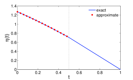
If $t$ is small, then we can approximate $m\approx 1/t$, from which the series expansion of ${\rm ctan}(x)$ leads to

$$\eta(t)\approx\frac{4}{\pi}-t-\frac{\pi}{12}~{}t^{2}+O(t^{3})\qquad(t<0.5).$$ (58)

This expansion accurately approximates the function $\eta(t)$ for $t<0.5$, as illustrated on Fig. 7. For $t>0.5$, one has $m=1$, and Eq. (A.2) simplifies to $\eta(t)=\sqrt{2}(1-t)$, while Eq. (54) is reduced to Eq. (8).

Figure 7: (Color online) The function $\eta(t)$ and its approximation (58) for $t<0.5$. For $t>0.5$, one has the exact relation $\eta(t)=\sqrt{2}(1-t)$.

A.3 The case $1/3<t<1/2$

For the case $1/3<t<1/2$ ($m=2$), one performs the computation analytically and gets the following result

$$\varphi_{t}(s)=\frac{\exp\left(-\frac{g}{2}\left[(1-2t)(1+\sqrt{3})+(3t-1)\sqrt{2}\right]\right)}{(1+\tilde{q}_{1})(1+\tilde{q}_{2})(1+q_{1})\sqrt{c_{0}+gc_{1}}},$$ (59)

where

$$c_{0}(g) = \frac{1}{576}\biggl{(}9+4\sqrt{3}\tilde{\alpha}_{1}\tilde{\alpha}_{2}+10\sqrt{6}\tilde{\alpha}_{2}\alpha_{1}+\tilde{\alpha}_{1}^{2}\tilde{\alpha}_{2}^{2}+16\tilde{\alpha}_{2}^{2}\alpha_{1}^{2}+6\sqrt{2}\tilde{\alpha}_{1}\alpha_{1}\tilde{\alpha}_{2}^{2}\biggr{)},$$

$$c_{1}(g) = \frac{5t-1}{576}\biggl{(}6\tilde{\alpha}_{1}+\frac{3}{\sqrt{2}}\tilde{\alpha}_{1}^{2}\tilde{\alpha}_{2}^{2}\alpha_{1}+6\tilde{\alpha}_{1}\tilde{\alpha}_{2}^{2}\alpha_{1}^{2}+2\sqrt{3}\tilde{\alpha}_{2}\alpha_{1}^{2}+\frac{3}{\sqrt{2}}\alpha_{1}+6\sqrt{6}\tilde{\alpha}_{1}\tilde{\alpha}_{2}\alpha_{1}+2\sqrt{3}\tilde{\alpha}_{1}^{2}\tilde{\alpha}_{2}\biggr{)}.$$

It is worth recalling that the “coefficients” $c_{0}$ and $c_{1}$, as well as $\tilde{q}_{1}$, $\tilde{q}_{2}$, $q_{1}$, $\tilde{\alpha}_{1}$, $\tilde{\alpha}_{2}$, $\alpha_{1}$ all depend on $g$ which enters through an exponential function. As $t$ gets smaller, expressions are getting even more cumbersome.

A.4 Exact formulas for $t=1/3$ and $t=1/4$

For the case $t=1/m$ with small $m=2,3,4,...$, the matrix $\mathbf{A}$ from Eq. (49) has a small size so that one can compute $\det(\mathbf{A})$ explicitly. For instance, one has for $m=3$,

$$\det(\mathbf{A})=\frac{g^{2}}{12\alpha_{1}\alpha_{2}}\biggl{[}4g\sqrt{3}\alpha_{1}+4g\alpha_{2}\alpha_{1}^{2}+\alpha_{1}^{2}\alpha_{2}^{2}\sqrt{3}+9\sqrt{3}+12\alpha_{1}\alpha_{2}\biggr{]},$$

and for $m=4$

$$\det(\mathbf{A}) = \frac{g^{3}}{64\alpha_{1}\alpha_{2}\alpha_{3}}\biggl{[}-4g\alpha_{2}^{2}\alpha_{3}^{2}\alpha_{1}\sqrt{2}\nu_{1}+12g\alpha_{2}^{2}\alpha_{3}\alpha_{1}^{2}\nu_{1}\sqrt{2}-32\alpha_{2}\alpha_{3}\nu_{1}\sqrt{2}$$

$$+128\alpha_{1}\alpha_{2}\sqrt{2}\nu_{1}+12\sqrt{2}g\nu_{1}\alpha_{3}+28g\alpha_{1}\sqrt{2}\nu_{1}+8g\alpha_{2}^{2}\alpha_{3}^{2}\alpha_{1}\nu_{1}$$

$$+16g\alpha_{2}^{2}\alpha_{3}\alpha_{1}^{2}\nu_{1}+160\alpha_{1}\alpha_{2}\nu_{1}+96\nu_{1}\alpha_{2}\alpha_{3}+40g\alpha_{1}\nu_{1}-16g\nu_{1}\alpha_{3}$$

$$-16\alpha_{2}^{2}\sqrt{2}\alpha_{3}^{2}+16\alpha_{2}^{2}\alpha_{1}^{2}\sqrt{2}+16\alpha_{1}\alpha_{2}^{2}\sqrt{2}\alpha_{3}+17g\alpha_{2}\alpha_{3}^{2}\sqrt{2}$$

$$+17g\alpha_{1}^{2}\alpha_{2}\sqrt{2}+64+24\alpha_{2}^{2}\alpha_{3}^{2}+24\alpha_{2}^{2}\alpha_{1}^{2}+24g\alpha_{1}^{2}\alpha_{2}-24g\alpha_{2}\alpha_{3}^{2}+12g\alpha_{2}\alpha_{3}\alpha_{1}\biggr{]},$$

where $\nu_{1}=\sqrt{\mu_{1}}/2=\sin(\pi/8)=\sqrt{2-\sqrt{2}}/2$. For larger $m$, explicit formulas are much more cumbersome.

Appendix B Cumulant moments

The simple explicit formula (8) for $\varphi_{t}(s)$ allows one to easily compute high-order cumulant moments of $\chi_{t}$ for $t>\frac{1}{2}$. The analysis of the opposite case $t<\frac{1}{2}$ is more difficult, especially for small $t$. For this reason, we present an alternative approach to evaluation of these moments.

We start by establishing a formal representation of $\varphi_{t}(s)$ as a determinant of some integral operator. Using the standard Gaussian identity

$$e^{-x^{2}/2}=\int\limits_{\mathbb{R}}\frac{dy}{\sqrt{2\pi}}~{}e^{-y^{2}/2+ixy},$$

one can rewrite Eq. (5) by introducing an auxiliary Gaussian field $Y$:

$$\varphi_{t}(s) = \int\mathcal{D}Y(u)\exp\left(-\frac{1}{2}\int\limits_{0}^{1-t}Y^{2}(u)\right)\int\limits_{\mathbb{R}}dx_{1}\int\limits_{X(0)=0}^{X(1)=x_{1}}\mathcal{D}X(u)$$

$$\times\exp\left(-\frac{1}{2}\int\limits_{0}^{1}(\partial_{u}X(u))^{2}+i\left(\frac{2s}{1-t}\right)^{1/2}\int\limits_{0}^{1-t}Y(u)(X(u+t)-X(u))\right).$$

Splitting the trajectory $X(u)$ into a linear part $tx_{1}$ and Brownian bridge $\tilde{X}(u)$ started from $0$ and arrived at $0$ at time $t=1$, one integrates over the whole path $X(u)$ to get

$$\varphi_{t}(s)=\int\mathcal{D}Y(u)\exp\left(-\frac{1}{2}\int\limits_{0}^{1-t}duY^{2}(u)-\frac{s}{1-t}\int\limits_{0}^{1-t}du\int\limits_{0}^{1-t}dv~{}Y(u)G(u,v)Y(v)\right),$$

where $G(u,v)$ is a combination of the two-point correlators $C(u,v)$ of Brownian bridge $\tilde{X}(u)$

$$C(u,v) = (1-v)u-(u-v)\Theta(u-v),$$

$$G(u,v) = t^{2}+C(u+t,v+t)-C(u+t,v)-C(u,v+t)+C(u,v),$$

where $\Theta(x)$ is the Heaviside function: $\Theta(x)=1$ for $x>0$ and $0$ otherwise. One gets then

$$G(u,v)=(u-v+t)\Theta(u-v+t)+(u-v-t)\Theta(u-v-t)-2(u-v)\Theta(u-v),$$ (60)

which also reduces to $t-|u-v|$ for $|u-v|<t$, and $0$ otherwise.

Evaluating Gaussian integrals over the auxiliary field $Y(u)$ yields

$$\varphi_{t}(s)=\frac{1}{\sqrt{\det\left(1+\frac{2s}{1-t}G\right)}},$$

where $G$ is an integral operator with the kernel $G(u,v)$ acting from $L_{2}([0,1-t])$ to $L_{2}([0,1-t])$. This is a direct extension of the classical representation (as Eq. (30)) for discrete Gaussian processes to the continuous case (see [37]). Rewriting the above formula as

$$-\ln\varphi_{t}(s)=\frac{1}{2}\Tr\ln\left(1+\frac{2sG}{1-t}\right)=\frac{1}{2}\sum\limits_{n=1}^{\infty}\frac{1}{n}\left(\frac{-2s}{1-t}\right)^{n}\Tr(G^{n}),$$

one gets a representation of cumulant moments:

$$\kappa_{n}=(-1)^{n-1}\lim\limits_{s\to 0}\left(\frac{\partial^{n}\ln\varphi_{t}(s)}{\partial s^{n}}\right)=\frac{2^{n-1}(n-1)!}{(1-t)^{n}}\Tr(G^{n}).$$

More explicitly, one has

$$\kappa_{n}=\frac{2^{n-1}(n-1)!}{(1-t)^{n}}\int\limits_{0}^{1-t}du_{1}...\int\limits_{0}^{1-t}du_{n}~{}G_{u_{1},u_{2}}~{}G_{u_{2},u_{3}}~{}...~{}G_{u_{n},u_{1}},$$ (61)

with an explicit function $G_{uv}$ from (60).

Appendix C Large $g$ asymptotic behavior for $t<\frac{1}{2}$

C.1 Case $t=1/m$: representation of the determinant

In this section, we only consider the case $t=1/m$, with $m=2,3,4,...$, although the general situation could be analyzed in a similar way. The matrix $\mathbf{U}$ from Eq. (47) can be split into two parts: $\mathbf{U}=\mathbf{U}_{0}+g\,\mathbf{U}_{1}$, where the matrix $\mathbf{U}_{0}$ has only 4 nonzero elements which do not depend on $g$:

$$\mathbf{U}_{0}=\left(\begin{array}[]{c c c c c c}u_{0}^{+}&...&0&u_{0}^{-}&...&0\\ ...&...&...&...&...&...\\ 0&...&0&0&...&0\\ u_{0}^{-}&...&0&u_{0}^{+}&...&0\\ ...&...&...&...&...&...\\ 0&...&0&0&...&0\\ \end{array}\right),\qquad\mathbf{U}_{1}=g^{-1}(\mathbf{U}-\mathbf{U}_{0}).$$

Given that $\Psi_{0k}=1/\sqrt{m}$ and $u_{0}^{+}=-u_{0}^{-}=1/t=m$, one finds

$$\mathbf{A}_{0}=\mathbf{V}^{T}\mathbf{U}_{0}\mathbf{V}=\left(\begin{array}[]{c c c c}0&...&0&0\\ ...&...&...&...\\ 0&...&0&0\\ 0&...&0&1\\ \end{array}\right).$$

One has therefore

$$\det(\mathbf{A})=\det(\mathbf{A}_{0}+g\,\mathbf{A}_{1})=\det(\mathbf{A}_{1})\det(g\mathbf{I}+\mathbf{A}_{1}^{-1}\mathbf{A}_{0})=\det(\mathbf{A}_{1})\prod\limits_{k=1}^{m}(g+\alpha_{k}),$$

where $\mathbf{A}_{1}=\mathbf{V}^{T}\mathbf{U}_{1}\mathbf{V}$ and $\alpha_{k}$ are the eigenvalues of the matrix $\mathbf{A}_{1}^{-1}\mathbf{A}_{0}$. Since the matrix $\mathbf{A}_{0}$ has only one nonzero element, the product $\mathbf{A}_{1}^{-1}\mathbf{A}_{0}$ is a matrix in which only the last column is nonzero. As a consequence, all the eigenvalues of this product are zero, except one, which is equal to $(\mathbf{A}_{1}^{-1})_{m-1,m-1}$. We obtain therefore

$$\det(\mathbf{A})=\det(\mathbf{A}_{1})g^{m-1}(g+(\mathbf{A}_{1}^{-1})_{m-1,m-1})=g^{m-1}(a_{0}+a_{1}g),$$ (62)

where the coefficients $a_{0}=\det(\mathbf{A}_{1})(\mathbf{A}_{1}^{-1})_{m-1,m-1}$ and $a_{1}=\det(\mathbf{A}_{1})$ depend on $g$ only through the coefficients $\alpha_{k}$ in the matrix $\mathbf{A}_{1}$. Denoting

$$c_{i}=\frac{a_{i}}{m2^{m-1}}\prod\limits_{k=1}^{m-1}\frac{\alpha_{k}}{\sqrt{\lambda_{k}}}\qquad(i=0,1),$$

one gets $I_{t}(g)=c_{0}+gc_{1}$ so that

$$\varphi_{t}(s)=\frac{\exp\left(-\frac{g}{2}t\sum\limits_{k=1}^{m-1}\sqrt{\lambda_{k}}\right)}{(1+q_{1})...(1+q_{m-1})\sqrt{c_{0}+gc_{1}}}.$$

This representation is exact but quite formal as the dependence on $g$ and $t$ is still “hidden” in coefficients $c_{0}$ and $c_{1}$.

C.2 Case $t=1/m$: large $g$ asymptotic behavior

For large $g$, all $\alpha_{k}$ are close to $1$, while $q_{k}$ are negligible so that

$$c_{i}\simeq\frac{a_{i}}{m^{3/2}2^{m-1}}\qquad(g\gg 1,~{}i=0,1),$$ (63)

where we used the identity

$$\prod\limits_{k=1}^{m-1}\sqrt{\lambda_{k}}=\prod\limits_{k=1}^{m-1}2\sin(\frac{\pi k}{2m})=\sqrt{m}.$$ (64)

Since the coefficients $a_{i}$ depend on $g$ only through $q_{k}$, they rapidly converge to the limiting values. In the limit $g\to\infty$, the matrix $\mathbf{U}_{1}$ gets a diagonal form

$$\mathbf{U}_{1}\simeq\left(\begin{array}[]{c | c}\sqrt{\mathbf{\Lambda}}&0\\ \hline\cr 0&\sqrt{\mathbf{\Lambda}}\\ \end{array}\right),$$

from which

$$\mathbf{A}_{1}=\mathbf{V^{T}}\mathbf{U}_{1}\mathbf{V}\simeq\mathbf{V}^{T}\sqrt{\mathbf{\Lambda}}\mathbf{V}+\mathbf{S}^{T}\mathbf{V}^{T}\sqrt{\mathbf{\Lambda}}\mathbf{V}\mathbf{S}=\sqrt{\mathbf{L}}+\mathbf{S}^{T}\sqrt{\mathbf{L}}\mathbf{S}\qquad(g\gg 1).$$

The limiting matrix on the right-hand side, which is explicit and independent of $g$, determines the limiting values $a_{0}$ and $a_{1}$. Moreover, the explicit formulas for $\lambda_{k}$ and $\Psi_{kl}$ allow one to get the elements of the matrix $\sqrt{\mathbf{L}}$ ($k,l=0,...,m-1$):

$$(\sqrt{\mathbf{L}})_{kl}=-\frac{\sin(\frac{\pi}{2m})}{m}\left(\frac{1}{\cos(\frac{\pi}{2m})-\cos(\frac{\pi(k-l)}{m})}+\frac{1}{\cos(\frac{\pi}{2m})-\cos(\frac{\pi(k+l+1)}{m})}\right).$$

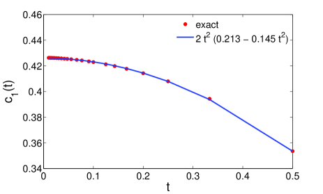
Using this representation, we obtain numerically an accurate approximation

$$a_{1}=\det(\mathbf{A}_{1})\simeq\sqrt{t}~{}2^{m}~{}(0.213-0.145t^{2}+...),$$

from which

$$c_{1}(t)\simeq\frac{a_{1}}{m^{3/2}2^{m-1}}=2t^{2}(0.213-0.145t^{2}+...).$$ (65)

Its accuracy is illustrated on Fig. 8.

Figure 8: (Color online) The exact coefficient $c_{1}(t)$ for $m=2,...,101$ computed through Eq. (63) and its fit as $2t^{2}(0.213-0.145t^{2})$.

C.3 General case

In the general case $\frac{1}{m+1}<t<\frac{1}{m}$ (for some $m=2,3,4,...$), the analysis is quite similar but formulas are more cumbersome. The contribution $I_{t}(g)$ from the Gaussian integral reads as

$$I_{t}(g)=\frac{\delta(t-\delta)}{2^{2m-3}g^{2m-1}\sqrt{m(m+1)}}\det(\mathbf{A}).$$

By construction, the matrix $\mathbf{A}$ can be represented as $\mathbf{A}=\mathbf{A}_{0}+g\mathbf{A}_{1}$, where the matrix $\mathbf{A}_{0}$ is independent of $g$, while the matrix $\mathbf{A}_{1}$ depends on $g$ only through $\alpha_{k}$ and $\tilde{\alpha}_{k}$. As a consequence, $\mathbf{A}_{1}$ becomes independent of $g$ for large $g$ (or $s$). The determinant of the matrix $\mathbf{A}_{0}+g\mathbf{A}_{1}$ is in general a polynomial of $g$ of degree $2m+1$. We conclude that the asymptotic behavior of $\varphi_{t}(s)$ in Eq. (10) is essentially determined by the exponential function $\exp(-\sqrt{s}\frac{\eta(t)}{\sqrt{2(1-t)}})$, with an algebraic prefactor from $\det(\mathbf{A})$.

For the cases $m=1$ and $m=2$, we obtain that $\det(\mathbf{A})=g^{2m-1}(a_{0}+a_{1}g)$, with the coefficients $a_{0}$ and $a_{1}$ depending on $t$. As a consequence, one gets $I_{t}(g)=c_{0}+c_{1}g$, with the new coefficients $c_{0}$ and $c_{1}$. We expect that this representation is valid for any $m$, but the related analysis is beyond the scope of the paper.

Appendix D Small $g$ asymptotic behavior for $t<\frac{1}{2}$

We only consider the specific cases $t=1/m$, with $m=2,3,4,...$. One can split the explicit representation (49) into two parts: $\mathbf{A}=\mathbf{H}_{0}+\mathbf{H}_{1}$, with

$$\mathbf{H}_{0}=\frac{g\sqrt{\mathbf{L}}}{\tanh(gt\sqrt{\mathbf{L}})},\quad\mathbf{H}_{1}=-\mathbf{S}^{T}\frac{g\sqrt{\mathbf{L}}}{\sinh(gt\sqrt{\mathbf{L}})}-\frac{g\sqrt{\mathbf{L}}}{\sinh(gt\sqrt{\mathbf{L}})}\mathbf{S}+\mathbf{S}^{T}\frac{g\sqrt{\mathbf{L}}}{\tanh(gt\sqrt{\mathbf{L}})}\mathbf{S}.$$ (66)

One gets then $\det(\mathbf{A})=\det(\mathbf{H}_{0})\det(\mathbf{I}+\mathbf{H}_{0}^{-1}\mathbf{H}_{1})$, from which the explicit computation of the determinant $\det(\mathbf{H}_{0})$ yields

$$\varphi_{t}(s)=\exp\left(-\frac{gt}{2}\sum\limits_{k=1}^{m-1}\sqrt{\lambda_{k}}\right)\left(\prod\limits_{k=1}^{m-1}\frac{1+q_{k}^{2}}{2}\right)^{-1/2}~{}\frac{1}{\sqrt{\det(\mathbf{I}+\mathbf{H}_{0}^{-1}\mathbf{H}_{1})}}.$$ (67)

Up to this point, this is just another representation of the previous result.

In the limit $g\to 0$, one can expand $q_{k}$ from Eq. (43) into Taylor series to get

$$\ln\left(\prod\limits_{k=1}^{m-1}\frac{1+q_{k}^{2}}{2}\right)=\sum\limits_{k=1}^{m-1}\ln\left(\frac{1+q_{k}^{2}}{2}\right)\simeq-tg\sum\limits_{k=1}^{m-1}\sqrt{\lambda_{k}}+\frac{t^{2}g^{2}}{2}\sum\limits_{k=1}^{m-1}\lambda_{k}-\frac{t^{4}g^{4}}{12}\sum\limits_{k=1}^{m-1}\lambda_{k}^{2}+\cdots$$

Given that

$$\sum\limits_{k=1}^{m-1}\lambda_{k}=2(m-1),\qquad\sum\limits_{k=1}^{m-1}\lambda_{k}^{2}=6m-8,$$

one finds

$$\left(\prod\limits_{k=1}^{m-1}\frac{1+q_{k}^{2}}{2}\right)^{-1/2}\simeq\exp\left(\frac{gt}{2}\left(\sum\limits_{k=1}^{m-1}\sqrt{\lambda_{k}}\right)-st+\frac{s^{2}t^{3}(1-4t/3)}{(1-t)^{2}}+\cdots\right).$$

Note that the first term here exactly compensates the first factor in Eq. (67).

Now we turn to the analysis of the determinant $\det(\mathbf{I}+\mathbf{H}_{0}^{-1}\mathbf{H}_{1})$. Expanding expressions for $\mathbf{H}_{0}^{-1}$ and $\mathbf{H}_{1}$ from Eqs. (66) into Taylor series, one gets

$$\mathbf{H}_{0}^{-1}\mathbf{H}_{1} = (\mathbf{S}^{T}\mathbf{S}-\mathbf{S}^{T}-\mathbf{S})+\frac{z}{6}\biggl{(}2\mathbf{S}^{T}\mathbf{L}\mathbf{S}+\mathbf{S}^{T}\mathbf{L}+\mathbf{S}\mathbf{L}-2\mathbf{LS}^{T}\mathbf{S}+2\mathbf{LS}^{T}+2\mathbf{LS}\biggr{)}$$

$$-\frac{z^{2}}{90}\biggl{(}2\mathbf{S}^{T}\mathbf{L}^{2}\mathbf{S}+\frac{7}{4}(\mathbf{S}^{T}\mathbf{L}^{2}+\mathbf{L}^{2}\mathbf{S})+10\mathbf{LS}^{T}\mathbf{LS}+5\mathbf{LS}^{T}\mathbf{L}+5\mathbf{LSL}\biggr{)}+O(z^{3}),$$

where $z=g^{2}t^{2}$. Denoting $\mathbf{J}=\mathbf{I}+\mathbf{S}^{T}\mathbf{S}-\mathbf{S}^{T}-\mathbf{S}$, one has

$$\det(\mathbf{I}+\mathbf{H}_{0}^{-1}\mathbf{H}_{1})=\det(\mathbf{J})\det\left(\mathbf{I}+z\mathbf{J}_{1}+\frac{z^{2}}{2}\mathbf{J}_{2}+O(z^{3})\right),$$

where

$$\mathbf{J}_{1} = \frac{1}{6}\mathbf{J}^{-1}\biggl{(}2\mathbf{S}^{T}\mathbf{LS}+\mathbf{S}^{T}\mathbf{L}+\mathbf{SL}-2\mathbf{LS}^{T}\mathbf{S}+2\mathbf{LS}^{T}+2\mathbf{LS}\biggr{)},$$

$$\mathbf{J}_{2} = \frac{1}{45}\mathbf{J}^{-1}\biggl{(}2\mathbf{S}^{T}\mathbf{L}^{2}\mathbf{S}+\frac{7}{4}(\mathbf{S}^{T}\mathbf{L}^{2}+\mathbf{L}^{2}\mathbf{S})+10\mathbf{LS}^{T}\mathbf{LS}+5\mathbf{LS}^{T}\mathbf{L}+5\mathbf{LSL}\biggr{)}.$$

Checking that $\det(\mathbf{J})=1$ and using a perturbative expansion for the second determinant,

$$\det(\mathbf{I}+\mathbf{X})=1+\tr(\mathbf{X})+\frac{1}{2}\bigl{[}\tr(\mathbf{X})^{2}-\tr(\mathbf{X}^{2})\bigr{]}+\cdots,$$

one finds, up to $z^{2}$:

$$\det(\mathbf{I}+\mathbf{H}_{0}^{-1}\mathbf{H}_{1})=1+z\tr(\mathbf{J}_{1})+\frac{z^{2}}{2}\biggl{(}\tr(\mathbf{J}_{2})+(\tr(\mathbf{J}_{1}))^{2}-\tr(\mathbf{J}_{1}^{2})\biggr{)}+O(z^{3}).$$

Using the explicit form of the matrices $\mathbf{J}_{1}$ and $\mathbf{J}_{2}$, one can check that $\tr(\mathbf{J}_{1})=0$ and compute exactly two other traces, from which

$$\det(\mathbf{I}+\mathbf{H}_{0}^{-1}\mathbf{H}_{1})\simeq 1+s^{2}\frac{t^{3}(2/3-t)}{(1-t)^{2}}+O(s^{3}).$$ (68)

Bringing all these results together, we obtain

$$\varphi_{t}(s)\simeq e^{-ts}~{}\frac{\exp(s^{2}t^{3}\frac{(1-4t/3)}{(1-t)^{2}})}{\sqrt{1+s^{2}t^{3}\frac{2/3-t}{(1-t)^{2}}}}+O(s^{3}).$$ (69)

One can see that the factor in front of $e^{-ts}$ gives the second-order correction in the form $s^{2}t^{3}$. If one rescales the TAMSD $\chi_{t}$ by $t$ (to set the mean value to $1$), the Laplace transform $\tilde{\varphi}_{t}(s^{\prime})$ of the probability density for $\chi_{t}/t$ is obtained by replacing $st$ by $s^{\prime}$. In the limit $t\to 0$, one can show that $\tilde{\varphi}_{t}(s^{\prime})$ converges to $e^{-s^{\prime}}$, as expected.

Appendix E Comparison of moments

Given that a generalized Gamma distribution turns out to be an accurate approximation for the probability density $p_{t}(z)$, one can attempt to retrieve the parameters $a$, $b$ and $\nu$ of this distribution by matching the moments of the true and approximate distributions. For a GGD, one has

$$\mu_{\alpha}\equiv\langle\chi_{t}^{\alpha}\rangle=(ab)^{\alpha}\frac{K_{\nu+\alpha}(c)}{K_{\nu}(c)},\qquad c=2\sqrt{a/b}.$$ (70)

Following Ref. [37], one can solve the system of two nonlinear equations involving the first three moments:

$$\frac{\mu_{2}}{\mu_{1}^{2}}=\frac{K_{\nu+2}(c)K_{\nu}(c)}{K_{\nu+1}^{2}(c)},\qquad\frac{\mu_{3}}{\mu_{1}^{3}}=\frac{K_{\nu+3}(c)K_{\nu}^{2}(c)}{K_{\nu+1}^{3}(c)}.$$ (71)

Once the pair $\{c,\nu\}$ is found, one retrieves the other two parameters as

$$b=2\mu_{1}\frac{K_{\nu}(c)}{cK_{\nu+1}(c)},\qquad a=bc^{2}/4$$ (72)

(note that the first relation was misprinted in [37]). Using the explicit formulas (12), (13), (14) for the cumulant moments for $t<\frac{1}{2}$, one finds

$$\frac{\mu_{2}}{\mu_{1}^{2}} = 1+\frac{\kappa_{2}}{\kappa_{1}^{2}}=1+\frac{t(4-5t)}{3(1-t)^{2}}\simeq 1+\frac{4}{3}t+t^{2}+O(t^{3}),$$ (73)

$$\frac{\mu_{3}}{\mu_{1}^{3}} = 1+3\frac{\kappa_{2}}{\kappa_{1}^{2}}+\frac{\kappa_{3}}{\kappa_{1}^{3}}=1+\frac{t(60-69t-19t^{2})}{15(1-t)^{3}}\simeq 1+4t+\frac{37}{5}t^{2}+O(t^{3}).$$ (74)

We have solved numerically Eqs. (71) and found the dependence of the parameters $a$, $b$ and $\nu$ on the lag time $t$, as shown on Fig. 5.

One can see that when $t\to 0$, both $c$ and $\nu$ increase inversely proportional to $t$. In this limit, one can approximate the modified Bessel function $K_{\nu}(\nu x)$ as

$$K_{\nu}(\nu x)\simeq\sqrt{\pi/\nu}\left(\frac{1+\sqrt{1+x^{2}}}{x}\right)^{\nu}(1+x^{2})^{-1/4}e^{-\nu\sqrt{1+x^{2}}}.$$ (75)

Considering $\varepsilon=1/\nu$ as a small parameter and assuming $c/\nu$ to be a constant in the limit $t\to 0$, one takes $c/\nu=x-\alpha\varepsilon+\beta\varepsilon^{2}$ and gets

$$\frac{K_{\nu+2}(c)K_{\nu}(c)}{K_{\nu+1}^{2}(c)} \simeq 1+\frac{\varepsilon}{\sqrt{1+x^{2}}}+\Biggl{(}\frac{\alpha x}{(1+x^{2})^{3/2}}-\frac{\sqrt{1+x^{2}}-1}{(1+x^{2})^{2}}\Biggr{)}\varepsilon^{2}+O(\varepsilon^{3}),$$ (76)

$$\frac{K_{\nu+3}(c)K_{\nu}^{2}(c)}{K_{\nu+1}^{3}(c)} \simeq 1+\frac{3\varepsilon}{\sqrt{1+x^{2}}}+\Biggl{(}\frac{3\alpha x(2+\sqrt{1+x^{2}})}{(1+x^{2})(1+\sqrt{1+x^{2}})^{2}}$$

$$- \frac{2(2+x^{2})\sqrt{1+x^{2}}+3x^{4}+4x^{2}+4}{(1+x^{2})^{2}(1+\sqrt{1+x^{2}})^{2}}\Biggr{)}\varepsilon^{2}+O(\varepsilon^{3}).$$

It is worth noting that these terms are independent of $\beta$ (which appears in higher-order terms).

Comparing these expansions to Eqs. (73), (74), one sees that $\varepsilon$ is of the order of $t$. Taking $\varepsilon=\gamma t+\delta t^{2}+O(t^{3})$, one immediately gets $\gamma=\frac{4}{3}\sqrt{1+x^{2}}$ from the first-order terms. Substituting $\varepsilon=\frac{4}{3}\sqrt{1+x^{2}}~{}t+\delta~{}t^{2}$ into Eqs. (76), (E), one gets a system of two equations with three unknowns $\alpha$, $\delta$ and $x$:

$$\frac{\delta}{\sqrt{1+x^{2}}}+\Biggl{(}\frac{\alpha x}{\sqrt{1+x^{2}}}-\frac{\sqrt{1+x^{2}}-1}{(1+x^{2})}\Biggr{)}\frac{16}{9}=1,$$

$$\frac{3\delta}{\sqrt{1+x^{2}}}+\Biggl{(}\frac{3\alpha x(2+\sqrt{1+x^{2}})}{(1+\sqrt{1+x^{2}})^{2}}-\frac{2(2+x^{2})\sqrt{1+x^{2}}+3x^{4}+4x^{2}+4}{(1+x^{2})(1+\sqrt{1+x^{2}})^{2}}\Biggr{)}\frac{16}{9}=\frac{37}{5}.$$

These equations are linear in $\alpha$ and $\delta$. Expressing $\alpha$ from the first equation and substituting into the second one yields, after algebraic simplifications, a simple equation on $x$ which turns out to be independent of $\delta$: $2x^{2}-38+\sqrt{1+x^{2}}(21x^{2}-38)=0$. Its solution is

$$x=\frac{\sqrt{1159}}{21}\approx 1.6211.$$

As a consequence, one finds the leading terms for $\nu$ and $c$ and then for $a$ and $b$ as $t\to 0$ which are summarized in Eqs. (33), (34), (35).

References

- [1] Weiss G H, 1994 Aspects and Applications of the Random Walk (North-Holland, Amsterdam)
- [2] Ben-Avraham D and Havlin S, 2000 Diffusion and reaction in disordered systems (Cambridge University Press)
- [3] Saxton M J and Jacobson K, 1997 Annu. Rev. Biophys. Biomol. Struct. 26 373
- [4] Majumdar S N, 2005 Curr. Sci. 89 2076
- [5] Grebenkov D S, 2007 Rev. Mod. Phys. 79 1077
- [6] Bouchaud J-P and Potters M, 2000 Theory of Finantial Risks: From Statistical Physics to Risk Management (Cambridge University Press)
- [7] Qian H, Sheetz M P, and Elson E L, 1991 Biophys. J. 60 910
- [8] Saxton M J, 1993 Biophys. J. 64 1766
- [9] Saxton M J, 1997 Biophys. J. 72 1744
- [10] Goulian M and Simon S M, 2000 Biophys. J. 79 2188
- [11] Tolić-Norrelykke I M, Munteanu E-L, Thon G, Oddershede L, and Berg-Sorensen K, 2004 Phys. Rev. Lett. 93 078102
- [12] Golding I and Cox E C, 2006 Phys. Rev. Lett. 96 098102
- [13] Arcizet D, Meier B, Sackmann E, Rädler J O, and Heinrich D, 2008 Phys. Rev. Lett. 101 248103
- [14] Wilhelm C, 2008 Phys. Rev. Lett. 101 028101
- [15] Wirtz D, 2009 Ann. Rev. Biophys. 38 301
- [16] Metzler R, Tejedor V, Jeon J-H, He Y, Deng W H, Burov S, and Barkai E, 2009 Acta Phys. Pol. B 40 1315
- [17] Feynman R P and Hibbs A R, 1965 Quantum Mechanics and Path Integrals (New York, McGraw-Hill)
- [18] Freidlin M, 1985 Functional Integration and Partial Differential Equations, Annals of Mathematics Studies (Princeton University, Princeton, New Jersey)
- [19] Bray A J and Moore M A, 1980 J. Phys. C: Solid State Phys. 13 L655
- [20] Kirkpatrick T R and Thirumalai D, 1987 Phys. Rev. B 36 5388
- [21] Ruben H, 1962 Ann. Math. Stat. 33 542
- [22] Ruben H, 1963 Ann. Math. Stat. 34 1582
- [23] Robbins H, 1948 Ann. Math. Stat. 19 266
- [24] Robbins H and Pitman E J G, 1949 Ann. Math. Stat. 20 552
- [25] Pachares J, 1955 Ann. Math. Stat. 26 128
- [26] Shah B K and Khatri C G, 1961 Ann. Math. Stat. 32 883
- [27] Gurland J, 1953 Ann. Math. Stat. 24 416
- [28] Gurland J, 1955 Ann. Math. Stat. 26 122
- [29] Gurland J, 1956 Ind. J. Stat. 17 37
- [30] Kotz S, Johnson N L and Boyd D W, 1967 Ann. Math. Stat. 38 823
- [31] Kotz S, Johnson N L and Boyd D W, 1967 Ann. Math. Stat. 38 838.
- [32] Duits M H G, Li Y, Vanapalli S A, and Mugele F, 2009 Phys. Rev. E 79 051910
- [33] Boyer D and Dean D S, 2011 J. Phys. A: Math. Theor. 44 335003
- [34] Boyer D, Dean D S, Mejia-Monasterio C, and Oshanin G, 2012 Phys. Rev. E 85 031136
- [35] Voisinne G, Alexandrou A, and Masson J-B, 2010 Biophys. J. 98 596
- [36] Grebenkov D S, 2011 Phys. Rev. E 83 061117
- [37] Grebenkov D S, 2011 Phys. Rev. E 84 031124
- [38] Nakagawa K, 2007 IEEE Trans. Inf. Theory 53 3239
- [39] Hoel P G, 1962 Introduction to Mathematical Statistics (John Wiley and Sons, New York)