Y-system for $Y=0$ brane in planar AdS/CFT

Abstract

The spectrum of open strings with integrable $Y=0$ brane boundary conditions is analyzed in planar AdS/CFT. We give evidence that it can be described by the same Y-system that governs the spectrum of closed strings in ${\rm AdS}_{5}\times{\rm S}^{5}$, except with different asymptotic and analytical properties. We determine the asymptotic solution of the $Y$-system that is consistent both with boundary asymptotic Bethe ansatz and boundary Lüscher corrections.

1 Introduction

There have been recently immense interest and significant progress in applying integrable methods to the planar AdS/CFT correspondence, see Beisert:2010jr and references therein. The main focus has concerned the spectral problem, which aims to determine the scaling dimensions of gauge-invariant single-trace operators on one hand, and the energy levels of closed strings on the other. The sought-for spectrum can be encoded into the $Y$-system of the problem, which, when supplemented with the required asymptotical and analytical information, provides the unique physical solution.

In this paper we focus on the extension of the spectral problem to a case with boundary. Maximal giant gravitons McGreevy:2000cw ; Grisaru:2000zn correspond to baryonic (or determinant) operators in ${\cal N}=4$ super Yang-Mills (SYM) Balasubramanian:2001nh ; Corley:2001zk , and open strings ending on a maximal giant graviton brane correspond to determinant-like gauge-invariant operators Balasubramanian:2002sa ; deMelloKoch:2007uu . On the SYM side, Berenstein and Vázquez Berenstein:2005vf found the Hamiltonian of an open spin chain that gives the one-loop anomalous dimension of determinant-like operators in the scalar sector. They also determined the corresponding boundary S-matrix (or reflection matrix), and showed that it satisfies the boundary Yang-Baxter equation (BYBE) Cherednik:1985vs ; Sklyanin:1988yz ; Ghoshal:1993tm , suggesting that the model is integrable. (The double-row transfer matrix that generates the Berenstein-Vázquez Hamiltonian and the higher conserved charges was constructed and diagonalized only recently in Nepomechie:2011nz .) After some initial controversy Agarwal:2006gc ; Okamura:2006zr , Hofman and Maldacena Hofman:2007xp argued that integrability persists at two loops. As for bulk scattering, symmetry enhancement of the asymptotic spin chain offers a guide to finding the all-loop boundary S-matrix. For the so-called $Y=0$ brane, which is the simplest and most-studied example, $SU(1|2)^{2}$ symmetry determines the matrix part of the boundary S-matrix Hofman:2007xp (see Ahn:2008df for discussion on the BYBE). The scalar factor was found in Chen:2007ec by solving the boundary crossing and unitarity relations. The corresponding all-loop asymptotic Bethe ansatz (ABA) equations were studied in Galleas:2009ye . Based on Yangian symmetry of boundary scattering Ahn:2010xa ; MacKay:2010ey , bound-state boundary S-matrices were constructed in Ahn:2010xa ; Palla:2011eu . On the string theory side, integrable boundary conditions for sigma models and their flat connections were constructed in Mann:2006rh ; Dekel:2011ja . For a recent review including additional examples of boundaries, see Zoubos:2010kh .

The spectrum of open spin chains with finite length receives finite-size corrections, and the predictions of the boundary ABA equations are no longer reliable. The leading finite-size correction is due to virtual particles reflecting between the two boundaries, and their contribution can be described by a Lüscher-type formula Correa:2009mz ; Bajnok:2010ui . For the exact description, the contributions from higher virtual processes have to be summed up. In the periodic case, the sum of all virtual processes can be expressed by $Y$-functions which obey the $Y$-system.

The $Y$-system is a system of functional relations, which is related to the symmetry of the problem Zamolodchikov:1991et ; Kuniba:2010ir ; Gromov:2010kf . It encodes the group-theoretical fusion hierarchy of the transfer matrices in a gauge-invariant physical way. Usually it can be derived from an exact description of the problem, such as an integrable lattice realization (see e.g. Bazhanov:1987zu ; Kluemper1992304 ) or exact integral equations (TBA), which determine the finite-volume ground-state energy.

In the AdS/CFT setting, the $Y$-system was conjectured Gromov:2009tv based on the experience in relativistic models and by comparing its asymptotic solution to finite-size energy corrections Bajnok:2008bm . Later it was derived for the ground state from the thermodynamic Bethe ansatz equations Bombardelli:2009ns ; Gromov:2009bc ; Arutyunov:2009ur ; Arutyunov:2009ux . Excited-state TBA equations obtained by analytical continuation Dorey:1996re lead to the same $Y$-system. Although the scattering theory is invariant only under $SU(2|2)^{2}$, the spectrum has the full $PSU(2,2|4)$ symmetry. Indeed, it was shown in Gromov:2010vb (see also Arutyunov:2011uz ) that the conjectured $Y$-system exactly corresponds to this symmetry.

Introducing integrable boundary conditions in a model usually changes the asymptotic and analytical properties of the $Y$-functions, but not the $Y$-system. This is true for integrable lattice models with boundaries (see e.g. Behrend:1995zj ; OttoChui:2001xx ). It was conjectured and checked asymptotically that the $\beta$-deformed AdS/CFT correspondence can be described by the undeformed $Y$-system Gromov:2010dy . Later, using the model’s realization in terms of twisted boundary conditions Ahn:2010ws , the $Y$-system and the asymptotic and analytic information was derived from the ground-state TBA equations Ahn:2011xq (see also deLeeuw:2011rw ).

We expect that the $Y$-system used to describe the spectrum with periodical and twisted boundary conditions will persist to the boundary case with integrable boundary conditions. This expectation is also supported by the fact that the integrable boundary condition corresponding to a Wilson loop leads via a boundary TBA (BTBA) to the $Y$-system of $SU(2|2)$ Correa:2012hh ; Drukker:2012de . In this paper we focus on a different integrable boundary condition: the $Y=0$ brane Hofman:2007xp , which describes the dimension of determinant-like SYM operators such as

$${\cal O}_{Y}(Z^{k}\chi Z^{L-k})=\epsilon_{i_{1}\dots i_{N-1}i_{N}}^{j_{1}\dots j_{N-1}j_{N}}Y_{j_{1}}^{i_{1}}\dots Y_{j_{N-1}}^{i_{N-1}}(Z^{k}\chi Z^{L-k})_{j_{N}}^{i_{N}}\,.$$ (1.1)

Since in this case we do not have a BTBA equation for the ground state, we simply assume that the $Y$-system is not changed, and check the consistency of our assumption by direct computations of Lüscher corrections. We can thereby determine the relevant asymptotic and analytical solution, which is consistent with boundary Lüscher and asymptotic BA equations.

The paper is organized as follows: In the next Section 2 we review the $Y$-system of the planar $AdS_{5}/CFT_{4}$ correspondence. Then in Section 3 its asymptotic solution is determined in terms of the eigenvalues of the double-row transfer matrices. We construct a generating functional from which the bound-state transfer matrix eigenvalues can be extracted. We use these quantities to calculate the leading finite-size corrections of some operators and compare to the literature with confirmation in Section 4. Finally, we conclude in Section 5. Some details of the calculations, together with the implementation of the duality on the asymptotic BA and transfer matrices, are relegated to the Appendices.

2 The $AdS_{5}/CFT_{4}$ Y-system

The planar $AdS_{5}/CFT_{4}$ correspondence can be described by an integrable field theory, which has the global symmetry $PSU(2,2|4)$. It is generally believed that the symmetry determines the Y-system Gromov:2009tv , which, when supplemented with analyticity properties Cavaglia:2010nm ; Balog:2011nm , determines the spectrum of the model.

The form of the $Y$-system is very general

$$\frac{Y_{a,s}^{+}Y_{a,s}^{-}}{Y_{a-1,s}Y_{a+1,s}}=\frac{(1+Y_{a,s+1})(1+Y_{a,s-1})}{(1+Y_{a-1,s})(1+Y_{a+1,s})}\,,$$ (2.1)

and various models depend on the configurations of the nontrivial $Y$-functions and the analytical properties in the generalized rapidity variable $u$, $f^{\pm}(u)=f(u\pm\frac{i}{2})$. The $PSU(2,2|4)$ symmetry of the planar AdS/CFT integrable model leads to a T-shaped fat hook Y-system in Figure 1:

Figure 1: $Y$-system for planar AdS/CFT. The non-trivial $Y_{a,s}$-functions are marked by circles, massive nodes with black. The vertical and horizontal axes correspond to $a$ and $s$, respectively.

Models sharing the same symmetry often correspond to the same $Y$-system. What is different is the analytical properties of the $Y$-functions. The $AdS_{5}/CFT_{4}$ integrable model is more complicated than relativistic theories and has the unusual dispersion relation Beisert:2005tm ; Dorey:2006dq

$$E_{Q}(p_{Q})=\sqrt{Q^{2}+16g^{2}\sin^{2}\frac{p_{Q}}{2}}\,,\qquad g=\frac{\sqrt{\lambda}}{4\pi}\,,$$ (2.2)

where $Q\in\mathbb{Z}_{+}$ denotes the type of the particles: $Q=1$ corresponds to the fundamental particle, while $Q>1$ correspond to bound states of $Q$ fundamental particles. The rapidity parameter $u$ parameterizes the energy and momentum as

$$E_{Q}(u)=Q+2ig\left(\frac{1}{x^{[Q]}}-\frac{1}{x^{[-Q]}}\right)\,,\qquad p_{Q}(u)=-i\log\frac{x^{[Q]}}{x^{[-Q]}}\,,$$ (2.3)

where

$$x(u)=\frac{u}{2g}+\sqrt{\frac{u}{2g}-1}\sqrt{\frac{u}{2g}+1}\,,\qquad f^{[n]}(u)=f(u+\frac{in}{2})\,.$$ (2.4)

The momentum $p=p_{Q}(u)$ and the rapidity $u$ will be used interchangeably to parametrize physical quantities. The shifts $f^{\pm}=f^{[\pm 1]}$ are always understood to be with respect to the rapidity parameter.

The energy and momentum live on the torus parametrized by rapidity, while the $Y$-functions live on more complicated Riemann surfaces of rapidity. The ground-state $Y$-functions can be constructed from the pseudo energies of the mirror TBA equations Bombardelli:2009ns ; Gromov:2009bc ; Arutyunov:2009ur . The mirror model can be obtained from the original one by a double Wick rotation Ambjorn:2005wa ; Arutyunov:2007tc , $p\to-i\tilde{\epsilon}$, $E\to-i\tilde{p}$, which amounts to using (2.3) with

$$x(u)=\frac{u}{2g}+i\sqrt{1-\frac{u^{2}}{4g^{2}}}\,.$$ (2.5)

With these kinematical variables, the energy of a fundamental multi-particle state with momenta $p_{k}$ can be expressed in terms of only the massive $Y$-functions, $Y_{Q}=Y_{Q,0}$, as

$$E(L)=\sum_{k}E_{1}(p_{k})-\sum_{Q=1}^{\infty}\int\frac{du}{2\pi}\partial_{u}\tilde{p}_{Q}\log(1+Y_{Q})\,.$$ (2.6)

The momenta are determined by the function $Y_{1}(p)$, analytically continued from (2.5) to (2.4), via the exact Bethe equation:

$$Y_{1}(p_{k})=-1\,.$$ (2.7)

We expect that this structure is valid for both the periodic and the boundary situation. The difference lies in the asymptotic behavior of the $Y$-functions, which we analyze in the next section. The integration domains are also different. In the periodic case we integrate over the whole line, while for the boundary case only over the half line.

3 Asymptotic solution of the Y-system

In this section we analyze the asymptotic large-volume solution of the $Y$-system.

3.1 The asymptotic solution in general

The Y-system can be solved in terms of the $T$-system:

$$T_{a,s}^{+}T_{a,s}^{-}=T_{a+1,s}T_{a-1,s}+T_{a,s+1}T_{a,s-1}\,,$$ (3.1)

as

$$Y_{a,s}=\frac{T_{a,s+1}T_{a,s-1}}{T_{a+1,s}T_{a-1,s}}\,.$$ (3.2)

The $T$-functions are well-defined up to gauge transformations $T_{a,s}\to g^{[\pm a\pm s]}T_{a,s}$, where the signs are not correlated. We shall look for the asymptotic solution for large volume. In this limit the massive nodes are small and the $T$-system of $PSU(2,2|4)$ splits into two copies of the $SU(2|2)$ $T$-systems with boundary conditions $T_{a,0}=1$ Gromov:2009tv . The small massive nodes at leading order are determined by the asymptotic solutions of the two $SU(2|2)$ wings as:

$$Y_{a,0}=\frac{\phi^{[-a]}}{\phi^{[a]}}T_{a,-1}T_{a,1}\,.$$ (3.3)

The unknown function $\phi$ can be fixed by comparing it to the Lüscher correction. In the periodic case we obtain Bajnok:2008bm ; Bajnok:2010ui

$$Y_{a,0}=e^{-\tilde{\epsilon}_{a}L}\mathbb{T}_{a}\,,$$ (3.4)

where $\mathbb{T}_{a}$ is an eigenvalue of the full transfer matrix with the charge $a$ auxiliary representation space and the $N$-fold tensor product of the fundamental representations, which by the usual abuse of notation we denote in the same way:

$$\mathbb{T}_{a}(p,\{p_{i}\})=\mbox{sTr}_{a}(\mathbb{S}_{aN}(p,p_{N})\dots\mathbb{S}_{a1}(p,p_{1}))\,,$$ (3.5)

where sTr means supertrace and $\mathbb{S}_{aj}$ denotes the full scattering matrix of the charge $a$ auxiliary and the $j$-th fundamental particle. We introduce the basis for the fundamental representation of $SU(2|2)\otimes SU(2|2)$ by

$$|(\alpha\dot{\alpha})\rangle=|\alpha\rangle\otimes|\dot{\alpha}\rangle,\qquad\alpha=1,2,3,4,\qquad\dot{\alpha}=\dot{1},\dot{2},\dot{3},\dot{4}.$$ (3.6)

Labels $1,2,\dot{1},\dot{2}$ are bosonic, while $3,4,\dot{3},\dot{4}$ are fermionic.

As the (fundamental) scattering matrix has a factorized $SU(2|2)\otimes SU(2|2)$ form

$$\mathbb{S}=S_{0}\,S\otimes\dot{S},\qquad{\rm or}\qquad\mathbb{S}_{(\alpha\dot{\alpha})(\gamma\dot{\gamma})}^{(\beta\dot{\beta})(\delta\dot{\delta})}=S_{0}\,S_{\alpha\gamma}^{\beta\delta}\otimes\dot{S}_{\dot{\alpha}\dot{\gamma}}^{\dot{\beta}\dot{\delta}}\,,$$ (3.7)

the transfer matrix factorizes as well

$$\mathbb{T}_{a}=t_{a}\,t_{a,1}\otimes\dot{t}_{a,1}\,,\qquad t_{a,1}(p\,;\{p_{i}\})=\mbox{sTr}(S_{aN}(p,p_{N})\cdots S_{a1}(p,p_{1}))\,,$$ (3.8)

and the normalization is

$$t_{a}=t_{1}^{[1-a]}t_{1}^{[3-a]}\dots t_{1}^{[a-3]}t_{1}^{[a-1]}\,,\qquad t_{1}=\prod_{i=1}^{N}S_{0}(p,p_{i})\,.$$ (3.9)

Comparing the asymptotic solution of the $T$-system to the Lüscher correction, we can conclude that the $SU(2|2)$ $T$-functions are the left/right $SU(2|2)$ transfer matrices, and that $\frac{\phi^{-}}{\phi^{+}}=\left(\frac{x^{-}}{x^{+}}\right)^{L}t_{1}$. Clearly, the fused $SU(2|2)$ transfer matrices $t_{a,1}$ satisfy the $T$-system relation; and together with $\phi$, provide the needed asymptotic solution in the periodic case Gromov:2009tv .

Let us now turn to the boundary case. Comparing the asymptotic solution with the boundary Lüscher correction Bajnok:2010ui , we find

$$Y_{a,0}=e^{-2\tilde{\epsilon}_{a}L}\mathbb{D}_{a}\,,$$ (3.10)

where we have to replace the single-row transfer matrix with the double-row transfer matrix Sklyanin:1988yz ; Murgan:2008fs :

$$\mathbb{D}_{a}(p,\{p_{i}\})=\mbox{Tr}_{a}(\mathbb{S}_{aN}(p,p_{N})\dots\mathbb{S}_{a1}(p,p_{1})\mathbb{R}_{a}^{-}(p)\mathbb{S}_{1a}(p_{1},-p)\dots\mathbb{S}_{Na}(p_{N},-p)\tilde{\mathbb{R}}_{a}^{+}(-p))\,.$$ (3.11)

We remind the reader that $S_{aj}$ and $S_{ja}$ act nontrivially only on the vector spaces labeled by $a$ and $j$, and act as identity on all the other spaces; see Figure 2.

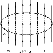
Figure 2: The double-row transfer matrix (3.11). The inner indices, represented by dashed lines in the figure, must also be summed.

Here $\mathbb{R}_{a}^{-}(p)$ denotes the full reflection factor of the charge $a$ particle on the right boundary. Note that the transfer matrix is not written in terms of the left reflection factor $\mathbb{R}_{a}^{+}(p)=\mathbb{R}_{a}^{-}(-p)$, but instead in terms of $\tilde{\mathbb{R}}_{a}^{+}(p)$. The latter is defined by

$$\mathbb{R}_{a}^{-}(p)\equiv\mbox{Tr}_{a^{\prime}}{\cal P}_{aa^{\prime}}\mathbb{S}_{aa^{\prime}}(p,-p)\,\tilde{\mathbb{R}}_{a^{\prime}}^{+}(-p),\\ {\rm or}\quad\mathbb{R}_{a}^{-}(p)_{(\gamma\dot{\gamma})}^{(\beta\dot{\beta})}=\mathbb{S}_{aa}(p,-p)_{(\alpha\dot{\alpha})(\gamma\dot{\gamma})}^{(\beta\dot{\beta})(\delta\dot{\delta})}\tilde{\mathbb{R}}_{a}^{+}(-p)_{(\delta\dot{\delta})}^{(\alpha\dot{\alpha})},$$ (3.12)

(where ${\cal P}$ is the permutation matrix), which ensures that $\mathbb{D}_{a}(p_{j},\{p_{i}\})$ is equal to the boundary Bethe-Yang matrix , and therefore $Y_{1,0}(p_{j})=-1$ is equivalent to the boundary Bethe-Yang equations. (See appendix A in Ahn:2000jd and Bajnok:2010ui for further details).

Factorization of the reflection factors

$$\mathbb{R}^{-}=R_{0}^{-}R^{-}\otimes\dot{R}^{-}\,,\qquad\tilde{\mathbb{R}}^{+}=\tilde{R}_{0}^{+}\tilde{R}^{+}\otimes\dot{\tilde{R}}^{+}\,,$$ (3.13)

together with the factorization of the scattering matrix implies the following factorization of the double-row transfer matrix

$$\mathbb{D}_{a}=d_{a}\,d_{a,1}\otimes\dot{d}_{a,1}\,,$$ (3.14)

where

$$d_{a,1}(p\,;\{p_{i}\})=\mbox{Tr}_{a}(S_{aN}(p,p_{N})\cdots S_{a1}(p,p_{1})R_{a}^{-}(p)S_{1a}(p_{1},-p)\dots S_{Na}(p_{N},-p)\tilde{R}^{+}_{a}(-p))\,,$$ (3.15)

and the normalization is

$$d_{a}=d_{1}^{[1-a]}d_{1}^{[3-a]}\dots d_{1}^{[a-3]}d_{1}^{[a-1]}\,,\qquad d_{1}=R_{0}^{-}(p)\tilde{R}_{0}^{+}(-p)\prod_{i=1}^{N}S_{0}(p,p_{i})S_{0}(p_{i},-p)\,.$$ (3.16)

Comparing the two expressions we can conclude that, in the boundary setting, the asymptotic solution of the $T$-system is

$$T_{a,1}=d_{a,1}\,,\qquad T_{a,-1}=\dot{d}_{a,1}\,,\qquad\frac{\phi^{-}}{\phi^{+}}=e^{-2\tilde{\epsilon}_{1}L}d_{1}\,.$$ (3.17)

As the calculation of the bound-state transfer matrices starting from the definition is very cumbersome, we turn to their generating functional. The generating functional is a compact solution of the $T$-system Kazakov:2007fy that is directly related to the fundamental transfer matrix. We start by calculating the generating functional for the $su(2)$ sector in the next subsection, and we then proceed with the general case.

3.2 The fundamental double-row transfer matrix

In this subsection we construct the fundamental $SU(2|2)$ double-row transfer matrix and explain its relation to the boundary asymptotic Bethe ansatz equations. In so doing we first fix our conventions. We normalize the fundamental scattering matrix (3.7) in the $su(2)$ compatible way Arutyunov:2006yd ; Arutyunov:2008zt :

$$S_{0}(x_{1},x_{2})=\frac{x_{1}^{+}+\frac{1}{x_{1}^{+}}-x_{2}^{-}-\frac{1}{x_{2}^{-}}}{x_{1}^{-}+\frac{1}{x_{1}^{-}}-x_{2}^{+}-\frac{1}{x_{2}^{+}}}\frac{x_{1}^{-}}{x_{1}^{+}}\frac{x_{2}^{+}}{x_{2}^{-}}\sigma^{2}(p_{1},p_{2})\,,\qquad S_{11}^{11}(x_{1},x_{2})=1=S_{\dot{1}\dot{1}}^{\dot{1}\dot{1}}(x_{1},x_{2})\,.$$ (3.18)

The reflection factor on the right boundary (3.13) is simply

$$R^{-}(p)=\dot{R}^{-}(p)=\mbox{diag}(e^{-i\frac{p}{2}},-e^{i\frac{p}{2}},1,1)\,,\qquad R_{0}^{-}(p)=-e^{-ip}\sigma(p,-p)\,.$$ (3.19)

The reflection factor on the left boundary is related to the right one as

$$\mathbb{R}^{+}(p)=\mathbb{R}^{-}(-p)\,.$$ (3.20)

Let us start to analyze a multiparticle state having particles of type $1\dot{1}$ only; see (3.6). The boundary asymptotic Bethe ansatz expresses the single-valuedness of the wave function:

$$e^{-2ip_{j}(L+1)}\prod_{k=j-1}^{1}S_{0}(p_{j},p_{k})R_{0}^{-}(p_{j})\prod_{k=1:k\neq j}^{N}S_{0}(p_{k},-p_{j})R_{0}^{-}(p_{j})\prod_{k=N}^{j+1}S_{0}(p_{j},p_{k})=1\,,$$ (3.21)

where the shift $L\rightarrow L+1$ is due to contributions from the matrix parts of the reflection matrices. For more general states one has to diagonalize the boundary Bethe-Yang matrix:

$$\prod_{k=j-1}^{1}\mathbb{S}_{jk}(p_{j},p_{k})\mathbb{R}^{-}_{j}(p_{j})\prod_{k=1:k\neq j}^{N}\mathbb{S}_{kj}(p_{k},-p_{j})\mathbb{R}^{+}_{j}(-p_{j})\prod_{k=N}^{j+1}\mathbb{S}_{jk}(p_{j},p_{k})\,.$$ (3.22)

Actually one has to diagonalize a family of such matrices obtained by moving each particle “around” the others by reflecting on both boundaries. This is done at once by defining the double-row transfer matrix of Sklyanin (3.11) with $a=1$, and there $\tilde{\mathbb{R}}_{1}^{+}(-p)$ was defined in such a way that $\mathbb{D}_{1}(p_{j},\{p_{i}\})$ gives back the boundary Bethe-Yang matrix (3.22). As both the scattering and reflection matrices factorize, we focus on one copy of the double-row transfer matrices. For concreteness, we normalize them as

$$\tilde{d}_{1,1}=\mbox{sTr}_{1}\left(S_{1N}(p,p_{N})\dots S_{11}(p,p_{1})R^{-}_{1}(p)S_{11}(p_{1},-p)\dots S_{N1}(p_{N},-p)R^{-}_{1}(-p)\right),$$ (3.23)

which differs from $d_{1,1}$ (3.15) since we used $R^{-}(-p)$ instead of $\tilde{R}^{+}(-p)$. They are related to each other due to the relation $R^{-}(-p)\propto(-1)^{F}\tilde{R}^{+}(-p)$, which changes the trace to supertrace. For later convenience, we record here that

$$\mathbb{D}_{1}(p)=\tilde{d}_{1}(p)\,\tilde{d}_{1,1}(p)\otimes\dot{\tilde{d}}_{1,1}(p)\,,$$ (3.24)

and note that the overall factor $\tilde{d}_{1}(p)$ will be determined in Section 4.

We first focus on the ground state eigenvalue of the transfer matrix $\tilde{d}_{1,1}(p)$ corresponding to $|1,1,\dots,1\rangle$. We show in Appendix B that the eigenvalue can be expressed in terms of only the diagonal part as

$$\Lambda^{su(2)}(p)=\rho_{1}\Lambda_{1}+\rho_{2}\Lambda_{2}-\rho_{3}\Lambda_{3}-\rho_{4}\Lambda_{4}\,,$$ (3.25)

where

$$\Lambda_{1} = R_{\ \,\,1}^{-1}(-p)S_{11}^{11}(p,p_{N})...S_{11}^{11}(p,p_{1})R_{\ \,\,1}^{-1}(p)S_{11}^{11}(p_{1},-p)...S_{11}^{11}(p_{N},-p)=1\,,$$ (3.26)

$$\Lambda_{2} = R_{\ \,\,2}^{-2}(-p)S_{21}^{21}(p,p_{N})...S_{21}^{21}(p,p_{1})R_{\ \,\,2}^{-2}(p)S_{12}^{12}(p_{1},-p)...S_{12}^{12}(p_{N},-p)=\frac{{\mathcal{R}}^{(-)+}}{{\mathcal{R}}^{(+)+}}\frac{{\mathcal{B}}^{(-)-}}{{\mathcal{B}}^{(+)-}}\,,$$

$$\Lambda_{3} = \Lambda_{4}=R_{\ \,\,3}^{-3}(-p)S_{31}^{31}(p,p_{N})...S_{31}^{31}(p,p_{1})R_{\ \,\,3}^{-3}(p)S_{13}^{13}(p_{1},-p)...S_{13}^{13}(p_{N},-p)=\frac{{\mathcal{R}}^{(-)+}}{{\mathcal{R}}^{(+)+}}\,,$$

and the functions ${\mathcal{B}}^{(\pm)},{\mathcal{R}}^{(\pm)}$ are defined in (A.2). The rapidity-dependent $\rho$ functions are

$$\rho_{1}=\frac{(1+(x^{-})^{2})(x^{-}+x^{+})}{2x^{+}(1+x^{+}x^{-})}\,,\quad\rho_{2}=\frac{x^{-}(x^{-}+x^{+})(1+(x^{+})^{2})}{2(x^{+})^{2}(1+x^{-}x^{+})}\,,\quad\rho_{3}+\rho_{4}=\frac{(x^{-}+x^{+})^{2}}{2(x^{+})^{2}}\,.$$ (3.27)

As $\Lambda_{3}$ and $\Lambda_{4}$ are the same, only the combination $\rho_{3}+\rho_{4}$ is determined.

Based on the analogy with the periodic theory Beisert:2005di ; Beisert:2006qh , we expect the generating functional of the eigenvalues of the transfer matrices for anti-symmetric representations to be of the form

$$\tilde{\mathcal{W}}^{-1} = (1-\mathcal{D}\rho_{1}\Lambda_{1}\mathcal{D})(1-\mathcal{D}\rho_{3}\Lambda_{3}\mathcal{D})^{-1}(1-\mathcal{D}\rho_{4}\Lambda_{4}\mathcal{D})^{-1}(1-\mathcal{D}\rho_{2}\Lambda_{2}\mathcal{D})$$ (3.28)

$$= \sum_{a}(-1)^{a}\mathcal{D}^{a}\tilde{d}_{a,1}\mathcal{D}^{a}\,,$$

where $\mathcal{D}=e^{-\frac{i}{2}\partial_{u}}$, and therefore $\mathcal{D}f=f^{-}\mathcal{D}$. In order to separate $\rho_{3}$ and $\rho_{4}$, we demand that the state without particles (${\mathcal{B}}^{(\pm)}={\mathcal{R}}^{(\pm)}=1$) corresponds to the BPS state ${\cal O}_{Y}(Z^{L})$, and thus all higher transfer matrices, $\tilde{d}_{a,1}$, vanish. This implies that

$$\tilde{\mathcal{W}}=1\quad\longrightarrow\quad\rho_{1}=\rho_{3}\,,\qquad\rho_{2}=\rho_{4}\,.$$ (3.29)

Let us renormalize the transfer matrices similarly to the periodic case by dividing by $\rho_{3}\Lambda_{3}$ as:

$$\mathcal{W}_{su(2)}^{-1} = (1-\mathcal{D}\frac{{\mathcal{R}}^{(+)+}}{{\mathcal{R}}^{(-)+}}\mathcal{D})(1-\mathcal{D}^{2})^{-1}(1-\mathcal{D}\frac{u^{+}}{u^{-}}\mathcal{D})^{-1}(1-\mathcal{D}\frac{u^{+}}{u^{-}}\frac{{\mathcal{B}}^{(-)-}}{{\mathcal{B}}^{(+)-}}\mathcal{D})$$ (3.30)

$$= \sum_{a}(-1)^{a}\mathcal{D}^{a}\hat{d}_{a,1}\mathcal{D}^{a}\,,$$

where we used that $\frac{\rho_{2}}{\rho_{1}}=\frac{\rho_{4}}{\rho_{3}}=\frac{u^{+}}{u^{-}}$ . The relation to $\tilde{d}_{a,1}$ is simply

$$\tilde{d}_{a,1}=f^{[a-1]}f^{[a-3]}\dots f^{[3-a]}f^{[1-a]}\hat{d}_{a,1}\,,\qquad f=\rho_{3}\Lambda_{3}\,.$$ (3.31)

Computing the generating functional, we found that

$$(-1)^{a}\hat{d}_{a,1}=(a+1)\rho_{B1}-a\rho_{F1}\frac{{\mathcal{R}}^{(+)[a]}}{{\mathcal{R}}^{(-)[a]}}-a\rho_{F2}\frac{{\mathcal{B}}^{(-)[-a]}}{{\mathcal{B}}^{(+)[-a]}}+(a-1)\rho_{B2}\frac{{\mathcal{R}}^{(+)[a]}}{{\mathcal{R}}^{(-)[a]}}\frac{{\mathcal{B}}^{(-)[-a]}}{{\mathcal{B}}^{(+)[-a]}}\,,$$ (3.32)

where

$$\rho_{B1}=\rho_{B2}=\frac{u}{u^{[-a]}}\,,\qquad\rho_{F1}=\frac{u^{-}}{u^{[-a]}}\,,\qquad\rho_{F2}=\frac{u^{+}}{u^{[-a]}}\,.$$ (3.33)

As we did not derive (3.28), but merely conjectured, we performed several consistency checks. First we analyzed $\hat{d}_{2,1}$. Using the explicit form of the bound-state scattering matrices and reflection factors we constructed the double-row transfer matrix $d_{a,1}$ of (3.15) for $a=2$ for $N=1,2,3$ particles at some randomly chosen momenta $p_{i}$ and coupling $g$. After verifying its commutativity properties, we diagonalized it and compared its eigenvalue to $\hat{d}_{2,1}.$ After restoring the correct normalization factor we obtained perfect agreement. We performed also another consistency check: we generated the double-row transfer matrices for symmetric representations as

$$\mathcal{W}_{su(2)}=\sum_{s}\mathcal{D}^{s}\hat{d}_{1,s}\mathcal{D}^{s}\,,$$ (3.34)

and in a similar fashion we checked explicitly $\hat{d}_{1,2}$.

3.3 Asymptotic Bethe ansatz and the generating functional

We now turn to the analysis of generic states. Following Guan:1990xx ; Galleas:2009ye and using experience with boundary systems, we expect the form of the generic eigenvalue of the double-row transfer matrix to be of the following dressed form:

$$\Lambda^{su(2)}=\left(\frac{x^{+}}{x^{-}}\right)^{m_{1}}\!\rho_{1}\frac{{\mathcal{R}}^{(-)+}}{{\mathcal{R}}^{(+)+}}\Biggr{[}\, \frac{{\mathcal{R}}^{(+)+}}{{\mathcal{R}}^{(-)+}}\frac{{\mathcal{B}}_{1}^{-}{\mathcal{R}}_{3}^{-}}{{\mathcal{B}}_{1}^{+}{\mathcal{R}}_{3}^{+}}-\frac{{\mathcal{B}}_{1}^{-}{\mathcal{R}}_{3}^{-}}{{\mathcal{B}}_{1}^{+}{\mathcal{R}}_{3}^{+}}\frac{Q_{2}^{++}}{Q_{2}}$$

$$-\frac{u^{+}}{u^{-}}\frac{{\mathcal{R}}_{1}^{+}{\mathcal{B}}_{3}^{+}}{{\mathcal{R}}_{1}^{-}{\mathcal{B}}_{3}^{-}}\frac{Q_{2}^{--}}{Q_{2}}+\frac{u^{+}}{u^{-}}\frac{{\mathcal{B}}^{(-)-}}{{\mathcal{B}}^{(+)-}}\frac{{\mathcal{R}}_{1}^{+}{\mathcal{B}}_{3}^{+}}{{\mathcal{R}}_{1}^{-}{\mathcal{B}}_{3}^{-}}\,\Biggl{]}\,,$$ (3.35)

where the notation (A.2), (A.3) is used. Regularity of the transfer matrix at the roots gives the boundary Bethe ansatz equations. Type $1$ roots are specified as $x^{+}(p)=y_{i}$, type $2$ roots when $u=w_{l}$, and in the boundary case type $3$ roots are equivalent to type $1$ roots: $x^{-}(p)=y_{i}^{-1}$. The corresponding Bethe equations read as

$$\frac{{\mathcal{R}}^{(+)+}Q_{2}}{{\mathcal{R}}^{(-)+}Q_{2}^{++}}\Bigg{|}_{x^{+}(p)=y_{i}}=1\,,\quad\frac{u^{-}}{u^{+}}\frac{Q_{1}^{-}Q_{2}^{++}}{Q_{1}^{+}Q_{2}^{--}}\Bigg{|}_{u=w_{l}}=-1\,,\quad\frac{{\mathcal{B}}^{(-)-}Q_{2}}{{\mathcal{B}}^{(+)-}Q_{2}^{--}}\Bigg{|}_{x^{-}(p)=y_{i}^{-1}}=1\,.$$ (3.36)

Note that the equations for $y_{i}$ following from the first and third sets of equations in (3.36) are the same. The second set of equations shows that the boundary factor $\frac{u^{-}}{u^{+}}$ can be removed formally by the redefinition $\tilde{Q}_{1}(u)\equiv u\,Q_{1}(u)$.

Let us describe their physical interpretation. Bethe ansatz equations diagonalize the scatterings and reflections in terms of massive particles ($\bullet$) and auxiliary “magnonic” particles. In the $SU(2|2)$ problem there are two types of magnons labelled by ${\sf y}$ and $\circ$. The massive node scatters on the magnons as

$$S_{\bullet{\sf y}}(p,y)=\frac{x^{-}-y}{x^{+}-y}\sqrt{\frac{x^{+}}{x^{-}}}\,,\quad S_{{\sf y}\bullet}(y,p)=\frac{y-x^{+}}{y-x^{-}}\sqrt{\frac{x^{-}}{x^{+}}}\,,\quad S_{\bullet\circ}(p,w)=1=S_{\circ\bullet}(w,p)\,,$$ (3.37)

the remaining scattering matrices are

$$S_{\circ\circ}(w_{1},w_{2})=\frac{w_{1}-w_{2}-i}{w_{1}-w_{2}+i}\,,\quad S_{{\sf y}\circ}(y,w)=S_{\circ{\sf y}}(y,w)=\frac{y+\frac{1}{y}-\frac{w}{g}+\frac{i}{2g}}{y+\frac{1}{y}-\frac{w}{g}-\frac{i}{2g}}\,,\quad S_{{\sf y}{\sf y}}(y_{1},y_{2})=1\,.$$ (3.38)

The boundary Bethe-Yang equations of the ${\sf y}$ magnons with parameter $y_{k}$ are

$$\prod_{j=1}^{N}S_{{\sf y}\bullet}(y_{k},p_{j})\prod_{l=1}^{m_{2}}S_{{\sf y}\circ}(y_{k},w_{l})R_{\sf y}^{-}(y_{k})\prod_{l=1}^{m_{2}}S_{\circ{\sf y}}(w_{l},-y_{k})\prod_{j=1}^{N}S_{\bullet{\sf y}}(p_{j},-y_{k})R_{\sf y}^{+}(-y_{k})=1\,.$$ (3.39)

Assuming that the reflection factors satisfy $R_{\sf y}^{-}(y)=R_{\sf y}^{+}(-y)$ and comparing to the Bethe ansatz equations (3.36), we can conclude that these reflection factors are equal to 1

$$R_{\sf y}^{\pm}(y)=1\,.$$ (3.40)

In a similar fashion, we can write the equations for the magnons $\circ$ with rapidity $w_{k}$:

$$\prod_{j=1:j\neq k}^{m_{1}}S_{\circ\circ}(w_{k},w_{j})\prod_{l=1}^{m_{2}}S_{\circ{\sf y}}(w_{k},y_{l})R_{\circ}^{-}(w_{k})\prod_{l=1}^{m_{2}}S_{{\sf y}\circ}(y_{l},-w_{k})\prod_{j=1:j\neq k}^{m_{1}}S_{\circ\circ}(w_{j},-w_{k})R_{\circ}^{+}(-w_{k})=1\,.$$ (3.41)

We assume also that the reflection factors satisfy $R_{\circ}^{-}(w)=R_{\circ}^{+}(-w)$ and compare to the Bethe ansatz equation (3.36). Naively we would think that $\frac{u^{-}}{u^{+}}$ corresponds to $R_{\circ}$; however, the $k=j$ term in the product for $Q_{2}$ cancels it completely, leading to

$$R_{\circ}^{\pm}(w)=1\,.$$ (3.42)

This is very similar to what has been obtained for the quark-antiquark potential problem Drukker:2012de ; Correa:2012hh .

The extension of the generating functional (3.30) for generic states reads as

$$\mathcal{W}_{su(2)}^{-1} = \left(1-\mathcal{D}\frac{{\mathcal{R}}^{(+)+}}{{\mathcal{R}}^{(-)+}}\frac{{\mathcal{B}}_{1}^{-}{\mathcal{R}}_{3}^{-}}{{\mathcal{B}}_{1}^{+}{\mathcal{R}}_{3}^{+}}\mathcal{D}\right)\left(1-\mathcal{D}\frac{{\mathcal{B}}_{1}^{-}{\mathcal{R}}_{3}^{-}}{{\mathcal{B}}_{1}^{+}{\mathcal{R}}_{3}^{+}}\frac{Q_{2}^{++}}{Q_{2}}\mathcal{D}\right)^{-1}\qquad\qquad\qquad$$

$$\qquad\qquad\times\left(1-\mathcal{D}\frac{u^{+}}{u^{-}}\frac{{\mathcal{R}}_{1}^{+}{\mathcal{B}}_{3}^{+}}{{\mathcal{R}}_{1}^{-}{\mathcal{B}}_{3}^{-}}\frac{Q_{2}^{--}}{Q_{2}}\mathcal{D}\right)^{-1}\left(1-\mathcal{D}\frac{u^{+}}{u^{-}}\frac{{\mathcal{B}}^{(-)-}}{{\mathcal{B}}^{(+)-}}\frac{{\mathcal{R}}_{1}^{+}{\mathcal{B}}_{3}^{+}}{{\mathcal{R}}_{1}^{-}{\mathcal{B}}_{3}^{-}}\mathcal{D}\right)$$

$$= \sum_{a}(-1)^{a}\mathcal{D}^{a}\hat{d}_{a,1}\mathcal{D}^{a}\,.$$

The relation to $\tilde{d}_{a,1}$ is again given by (3.31), except now

$$f=\rho_{1}\left(\frac{x^{+}}{x^{-}}\right)^{m_{1}}\frac{{\mathcal{R}}^{(-)+}}{{\mathcal{R}}^{(+)+}}\,.$$ (3.44)

It is straightforward to check that the transfer matrices constructed from the generating functional satisfy the $T$-system of $SU(2|2)^{2}$ (3.1).

4 Checking the Y-functions: the boundary Lüscher correction

We start by fixing the proper normalization of the double-row transfer matrix $\mathbb{D}$. To this end, we analyze single particle states. For a single particle the boundary Bethe-Yang equation reads as

$$1 = e^{-2ipL}\mathbb{R}^{+}(-p)\mathbb{R}^{-}(p)=e^{-2ipL}\mathbb{R}^{-}(p)^{2}$$

$$= e^{-2ipL}R_{0}^{-}(p)^{2}\mbox{diag}(e^{-ip},e^{ip},1,1)\otimes\mbox{diag}(e^{-ip},e^{ip},1,1)\,,$$

where we have used (3.19) and (3.20). In particular, for the $(1\dot{1})$ particle, we obtain (see also (3.21))

$$1=e^{-2ipL}R_{0}^{-}(p)^{2}e^{-2ip}=e^{-2ip(L+2)}\sigma^{2}(p,-p)\,,$$ (4.2)

which at leading order leads to the momentum quantization

$$p_{1\dot{1}}=\frac{\pi}{L+2}n\,,$$ (4.3)

where $n$ is an integer. The analogous equations for the $(2\dot{2})$ particle are

$$1=e^{-2ipL}\sigma^{2}(p,-p)\quad\longrightarrow\quad p_{2\dot{2}}=\frac{\pi}{L}n\,.$$ (4.4)

Let us recover the same result from the double-row transfer matrix. The fundamental transfer matrix with $N=1$ is given by (3.24), with

$$\tilde{d}_{1}(p)\equiv S_{0}(p,p_{1})S_{0}(p_{1},-p)\breve{R}_{0}^{+}(-p)R_{0}^{-}(p)\,,$$ (4.5)

where we have introduced the normalization factor $\breve{R}_{0}^{+}(-p)$ of the left reflection matrix that will be determined shortly. The boundary Bethe-Yang equation from the double-row transfer matrix is

$$\mathbb{D}_{1}(p_{1},\{p_{1}\})e^{-2ip_{1}L}=-1\,.$$ (4.6)

Comparing with (4.2), we see that

$$\mathbb{D}_{1}(p,\{p\})=-R_{0}^{-}(p)^{2}e^{-2ip}\,.$$ (4.7)

Note that $\mathbb{D}_{1}$ is diagonal; and the only nonvanishing contribution in the eigenvalue (3.25) of $\tilde{d}_{1,1}$ comes from the term with $\Lambda_{1}=1$. Using also that $S_{0}(p,p)=-1$ we obtain from (4.5)

$$\breve{R}_{0}^{+}(-p)=\frac{e^{-2ip}R_{0}^{-}(p)}{S_{0}(p,-p)\rho_{1}^{2}(p)}\equiv\frac{d_{0}(p)}{R_{0}^{-}(p)\rho_{1}^{2}(p)}\,,$$ (4.8)

where in the second equality we have introduced the new quantity $d_{0}(p)$. Having fixed the normalization of the left reflection factor, we now know the properly normalized double-row transfer matrix.

4.1 Lüscher correction

In the following we calculate the boundary Lüscher correction of a single impurity of type $(1\dot{1}$) and $(2\dot{2})$. These two states are in the $su(2)$ sector of the theory, and our transfer matrices are devised to calculate the correction to their energy. Correction to the energy of states of the form $(3\dot{3}$) or $(4\dot{4})$ can be easily calculated from the eigenvalues of the dual transfer matrices, which we obtain in Appendix C. The dualized transfer matrices are also relevant for deriving the BTBA equations since the bound states of the mirror theory are in the $sl(2)$ sectors.

The energies of the states $(1\dot{1}$) and $(2\dot{2})$ are no longer degenerate because the residual symmetry of the $Y=0$ brane is $SU(1|2)^{2}$. The properly normalized fundamental transfer matrix eigenvalue is (see (3.31), (4.5))

$$\mathbb{D}_{1}=f_{1,1}\hat{d}_{1,1}^{2}\,,$$ (4.9)

where

$$f_{1,1}=\tilde{d}_{1}\left(\rho_{3}\Lambda_{3}\right)^{2}=S_{0}(p,p_{1})S_{0}(p_{1},-p)d_{0}\left(\frac{{\mathcal{R}}^{(-)+}}{{\mathcal{R}}^{(+)+}}\right)^{2}\,.$$ (4.10)

Using the generating functional (3.30) we can generate the antisymmetric transfer matrices as

$$\mathbb{D}_{a}=f_{a,1}\hat{d}_{a,1}^{2}\,,\qquad f_{a,1}=f_{1,1}^{[a-1]}f_{1,1}^{[a-3]}\dots f_{1,1}^{[3-a]}f_{1,1}^{[1-a]}\,.$$ (4.11)

The Lüscher correction in terms of this transfer matrix is

$$\Delta E=-\sum_{a=1}^{\infty}\int\limits_{0}^{\infty}\frac{dq}{2\pi}\,\mathbb{D}_{a}\,e^{-2\tilde{\epsilon}_{a}L}\,,$$ (4.12)

where $q$ is the mirror momentum of the $a$-th auxiliary particle. This expression is exact at the leading order when the exponential ${\cal O}(e^{-2\tilde{\epsilon}_{a}L})$ is small, e.g. at weak coupling. We also expect that the Lüscher $\mu$-term is absent for fundamental particles at least in the weak-coupling limit Bajnok:2008bm . We now calculate it at leading order and compare to Bajnok:2010ui .

4.2 Weak-coupling expansion

To make contact with the “direct” computation of Bajnok:2010ui we use the parametrization

$$z^{[\pm a]}=\frac{q+ia}{4g}\left(\sqrt{1+\frac{16g^{2}}{q^{2}+a^{2}}}\pm 1\right)\,.$$ (4.13)

Then

$$\frac{{\mathcal{R}}^{(+)[a]}}{{\mathcal{R}}^{(-)[a]}} =\frac{z^{[a]}-x^{-}}{z^{[a]}-x^{+}}\frac{z^{[a]}+x^{+}}{z^{[a]}+x^{-}}=\frac{(q-2u+{i}(a+1))}{(q-2u+{i}(a-1))}\frac{(q+2u+{i}(a+1))}{(q+2u+{i}(a-1))}+\dots=\frac{Q^{[a+1]}}{Q^{[a-1]}}\,,$$

$$\frac{{\mathcal{B}}^{(-)[-a]}}{{\mathcal{B}}^{(+)[-a]}} =\frac{1-z^{[-a]}x^{+}}{1-z^{[-a]}x^{-}}\frac{1+z^{[-a]}x^{-}}{1+z^{[-a]}x^{+}}=\frac{(q-2u-{i}(a+1))}{(q-2u-{i}(a-1))}\frac{(q+2u-{i}(a+1))}{(q+2u-{i}(a-1))}+\dots=\frac{Q^{[-a-1]}}{Q^{[-a+1]}}\,.$$

As $d_{0}=e^{-2ip}\frac{u^{-}}{u^{+}}=\left(\frac{z^{-}}{z^{+}}\right)^{2}\frac{u^{-}}{u^{+}}$ for $Q=1$, we find

$$d_{0}^{[a-1]}d_{0}^{[a-3]}\dots d_{0}^{[3-a]}d_{0}^{[1-a]}=\left(\frac{z^{[-a]}}{z^{[a]}}\right)^{2}\frac{u^{[-a]}}{u^{[a]}}\,.$$ (4.14)

Similarly,

$$\frac{{\mathcal{R}}^{(-)+}}{{\mathcal{R}}^{(+)+}}=\frac{(q-2u)(q+2u)}{(q-2u+i)(q+2u+i)}+\dots\qquad\longrightarrow\qquad\frac{Q^{[1-a]}}{Q^{[1+a]}}\,,$$ (4.15)

and for the scalar factor

$$S_{0}(p,p_{1})S_{0}(p_{1},-p)=\left(\frac{z^{-}}{z^{+}}\right)^{2}\frac{Q^{[2]}}{Q^{[-2]}}\quad\longrightarrow\quad\left(\frac{z^{[-a]}}{z^{[a]}}\right)^{2}\frac{Q^{[a-1]}Q^{[a+1]}}{Q^{[1-a]}Q^{[-1-a]}}\,.$$ (4.16)

Collecting all factors, we obtain

$$f_{a,1}\simeq\left(\frac{z^{[-a]}}{z^{[a]}}\right)^{4}\frac{u^{[-a]}}{u^{[a]}}\frac{Q^{[a-1]}Q^{[1-a]}}{Q^{[a+1]}Q^{[-1-a]}}=\left(\frac{4g^{2}}{q^{2}+{a^{2}}}\right)^{4}\frac{q-{i}a}{q+{i}a}\frac{Q^{[a-1]}Q^{[1-a]}}{Q^{[a+1]}Q^{[-1-a]}}\,.$$ (4.17)

From eq.(3.32) the contribution of the matrix part is

$$\hat{d}_{a,1}\simeq\frac{(-1)^{a}2g^{2}}{q-ia}\left[\frac{2qa(q^{2}+a^{2}-1-4u^{2})(q^{2}+a^{2}+1+4u^{2})}{(q^{2}+a^{2})(1+4u^{2})Q^{[a-1]}Q^{[1-a]}}\right]\,.$$ (4.18)

Thus, the full contribution of the transfer matrix is

$$\mathbb{D}_{a}\simeq\frac{(4g^{2})^{6}}{(q^{2}+a^{2})^{5}}\left[\frac{qa(q^{2}+a^{2}-1-4u^{2})(q^{2}+a^{2}+1+4u^{2})}{(q^{2}+a^{2})(1+4u^{2})}\right]^{2}\frac{1}{Q^{[a+1]}Q^{[-1-a]}Q^{[a-1]}Q^{[1-a]}}\,.$$ (4.19)

To compute the Lüscher correction we need the weak-coupling limit $e^{-2\tilde{\epsilon}_{a}L}=\left(\frac{4g^{2}}{q^{2}+a^{2}}\right)^{2L}$. Then, for the $1\dot{1}$ particle, the leading Lüscher correction is

$$\Delta E=-\sum_{a=1}^{\infty}\int\limits_{0}^{\infty}\frac{dq}{2\pi}\frac{(4g^{2})^{2L+6}}{(q^{2}+a^{2})^{2L+5}}\left[\frac{qa([q^{2}+a^{2}]^{2}-[1+4u^{2}]^{2})}{(q^{2}+a^{2})(1+4u^{2})}\right]^{2}\frac{1}{Q^{[a+1]}Q^{[-1-a]}Q^{[a-1]}Q^{[1-a]}}\,.$$ (4.20)

For the $2\dot{2}$ particle the eigenvalue of the fundamental transfer matrix is related very simply to that of the $1\dot{1}$ particle: repeating the computation in Appendix B, it turns out that

$$\Lambda(p)_{2}^{su(2)}=e^{2ip}\left(\rho_{1}\Lambda_{1}+\rho_{2}\Lambda_{2}-\rho_{3}\Lambda_{3}-\rho_{4}\Lambda_{4}\right)\,.$$ (4.21)

This means that the higher transfer matrices for the $2\dot{2}$ case differ from the $1\dot{1}$ one only in their normalization $\mathbb{D}_{a}|_{2\dot{2}}=\left(\frac{z^{[a]}}{z^{[-a]}}\right)^{4}\mathbb{D}_{a}|_{1\dot{1}}$. Therefore, in the weak-coupling limit, for the $2\dot{2}$ particle the leading Lüscher correction can be written as

$$\Delta E=-\sum_{a=1}^{\infty}\int\limits_{0}^{\infty}\frac{dq}{2\pi}\frac{(4g^{2})^{2L+2}}{(q^{2}+a^{2})^{2L+1}}\left[\frac{qa([q^{2}+a^{2}]^{2}-[1+4u^{2}]^{2})}{(q^{2}+a^{2})(1+4u^{2})}\right]^{2}\frac{1}{Q^{[a+1]}Q^{[-1-a]}Q^{[a-1]}Q^{[1-a]}}\,.$$ (4.22)

To evaluate these expressions for the Lüscher corrections, we must set the $u$ parameter of the particle in question to the value that corresponds to one of the momentum values allowed by the boundary Bethe-Yang equations: $u=\cot(p_{n}/2)/2+o(g)$ as this guarantees that we are dealing with an eigenvalue of the double-row transfer matrix. With these $u$-s we compute the integrals in eq.(4.20, 4.22) by extending the integration domain to the whole real line and using the residue theorem, then we sum over $a$.

From Bajnok:2010ui we know that $L=2$ is the smallest possible value among non-BPS operators $\sim{\cal O}_{Y}(Z\,\Phi^{a\dot{a}}\,Z^{L-1})$; in this case for the $1\dot{1}$ particle we have (see 4.3)

$$1\dot{1}\qquad L=2\,:\qquad p_{n}=\{\frac{\pi}{4},\frac{\pi}{2},\frac{3\pi}{4}\}\,.$$ (4.23)

With these values we obtain

$$\Delta E_{1\dot{1}}(\frac{\pi}{2})=-2^{6}\cdot g^{20}\left(7\cdot 2^{5}\zeta(9)-429\cdot 2^{2}\zeta(13)+2431\zeta(17)\right)\,,$$ (4.24)

and (see Appendix D)

$$\Delta E_{1\dot{1}}(\frac{\pi}{4}) = -2^{5}\cdot g^{20}(-2^{3}\cdot 7\cdot(99-70\sqrt{2})\zeta(9)-2(6765-4785\sqrt{2})\zeta(11)$$

$$-2002(5\sqrt{2}-7)\zeta(15)+(7293-4862\sqrt{2})\zeta(17))\,,$$

$$\Delta E_{1\dot{1}}(\frac{3\pi}{4}) = -2^{5}\cdot g^{20}(-2^{3}\cdot 7\cdot(99+70\sqrt{2})\zeta(9)-2(6765+4785\sqrt{2})\zeta(11)$$ (4.25)

$$+2002(5\sqrt{2}+7)\zeta(15)+(7293+4862\sqrt{2})\zeta(17))\,.$$

For the $2\dot{2}$ particle with $L=2$ there is only one allowed $p$, namely $p=\frac{\pi}{2}$ (see 4.4), for which eq.(4.22) gives

$$\Delta E_{2\dot{2}}(\frac{\pi}{2})=-g^{12}\cdot 2^{6}\left(21\zeta(9)-3\cdot 2^{2}\zeta(5)\right)\,.$$ (4.26)

This expression coincides with the result of the direct Lüscher calculation based on the bound-state scattering and reflection matrices Bajnok:2010ui .

For $L=3$ the boundary Bethe-Yang equations give

$$2\dot{2}\qquad L=3\,:\qquad p_{n}=\{\frac{\pi}{3},\frac{2\pi}{3}\}\,,$$ (4.27)

and for the Lüscher correction we find

$$\Delta E_{2\dot{2}}(\frac{\pi}{3})=-g^{16}\cdot 2^{3}\left(15\zeta(7)-42\zeta(9)-165\zeta(11)+429\zeta(13)\right)\,.$$ (4.28)

$$\Delta E_{2\dot{2}}(\frac{2\pi}{3})=g^{16}\cdot 2^{3}\left(3645\zeta(7)+3402\zeta(9)-4455\zeta(11)-3861\zeta(13)\right)\,.$$ (4.29)

Comparing to the analogous computation in the periodic case for the Konishi operator Bajnok:2008bm , it is interesting to observe that all of these Lüscher corrections are given by linear combinations of zeta functions, and there are no “rational parts” (i.e. terms without zeta functions). Although we have no explanation, this is perhaps a generic feature of wrapping corrections for one-particle states (see also Fiamberti:2008sm ; Fiamberti:2008sn ; Gunnesson:2009nn ; Beccaria:2009hg ; Gromov:2010dy ). Also the leading Lüscher correction of the $2\dot{2}$ particle contains smaller powers of $g$ than that of the $1\dot{1}$, thus the “wrapping corrections” to the anomalous dimension of the corresponding operators appear in a lower loop order.

5 Conclusion

We showed in this paper that the $Y$-system can be used to analyze the spectral AdS/CFT problem in the boundary setting. We identified the asymptotic solution which was consistent both with boundary asymptotic Bethe ansatz and boundary Lüscher correction. Using this asymptotic solution we determined leading order wrapping corrections of various simple determinant-type operators.

In our approach we assumed that the $Y$-system is independent of the boundary condition, and indicated that its asymptotic solution satisfies the possible requirements. A more rigorous way would be to derive the ground-state BTBA equations from first principles (e.g. string hypothesis), and prove that the $Y$-functions as constructed from the pseudo-energies indeed satisfy the $Y$-system. The solutions of the $Y$-system equations have to satisfy excited-states BTBA equations. It would be an interesting project to transform the $Y$-system into BTBA equations based on the asymptotic solution that we have determined, similarly to the way it was done for the periodic case Cavaglia:2010nm ; Balog:2011nm .

We have explicitly constructed some bound-state double-row transfer matrices and checked that they indeed satisfy the functional relations of the $T$-system. We performed this task only for the first few transfer matrices where the bound-state scattering and reflection matrices were available. It would be nice to show decisively that they indeed satisfy the fusion hierarchy and can be analyzed in the fashion of Kazakov:2007fy .

In this paper we analyzed the $Y=0$ brane boundary condition. We expect that the same $Y$-system describes the finite-size spectrum of open strings with any other integrable boundary conditions. The asymptotic solutions could be extracted from the asymptotic BA equations Correa:2009dm ; Correa:2011nz .

Appendix A Notation

The $x$ variable is defined by

$$x(u)+\frac{1}{x(u)}=\frac{u}{g}\,,$$ (A.1)

and it has branch points at $u=\pm 2g$. As for the energy and momentum of string states, we choose the branch cut along $u\in(-2g,2g)$ as in (2.4). For the mirror particles, we choose the branch cut along $u\in(-\infty,-2g)\cup(2g,\infty)$ as in (2.5). There are two conventions for the mirror $x$ variable in the literature. We adopt the choice ${\rm Im}\,x>0$ in this paper, as used in e.g. Bajnok:2008bm ; Gromov:2009tv . The other choice ${\rm Im}\,x<0$ is used in e.g. Arutyunov:2009ur .

The eigenvalues of double-row transfer matrix are expressed through

$${\mathcal{R}}^{(\pm)}=\prod_{i=1}^{N}\left(x(p)-x^{\mp}(p_{i})\right)\left(x(p)+x^{\pm}(p_{i})\right)\,,\qquad Q(u)=\prod_{i=1}^{N}(u-u_{i})(u+u_{i})\,,$$

$${\mathcal{B}}^{(\pm)}=\prod_{i=1}^{N}\left(\frac{1}{x(p)}-x^{\mp}(p_{i})\right)\left(\frac{1}{x(p)}+x^{\pm}(p_{i})\right)\,,$$ (A.2)

for the $N$-particle ground state $|1,1,\dots,1\rangle$, and

$${\mathcal{B}}_{1}{\mathcal{R}}_{3}=\prod_{j=1}^{m_{1}}\left(x(p)-y_{j}\right)\left(x(p)+y_{j}\right)\,,\qquad{\mathcal{R}}_{1}{\mathcal{B}}_{3}=\prod_{j=1}^{m_{1}}\left(\frac{1}{x(p)}-y_{j}\right)\left(\frac{1}{x(p)}+y_{j}\right)\,,$$

$$Q_{1}(u)=\prod_{j=1}^{m_{1}}\left(\frac{u}{g}-y_{j}-\frac{1}{y_{j}}\right)\left(\frac{u}{g}+y_{j}+\frac{1}{y_{j}}\right)=\left(\prod_{j=1}^{m_{1}}-\frac{1}{y_{j}^{2}}\right){\mathcal{B}}_{1}{\mathcal{R}}_{3}{\mathcal{R}}_{1}{\mathcal{B}}_{3}\,,$$

$$Q_{2}(u)=\prod_{l=1}^{m_{2}}(u-w_{l})(u+w_{l})\,,$$ (A.3)

for generic states with auxiliary roots: $2m_{1}$ is the number of $y$-roots, and $2m_{2}$ is the number of $w$-roots.

Appendix B Vacuum eigenvalue

The open-chain transfer matrix for a single copy of $SU(2|2)$ in the fundamental representation is given by (3.23) Sklyanin:1988yz ; Murgan:2008fs , which we now write as

$$\tilde{d}_{1,1}(p\,;\{p_{i}\})=\mbox{sTr}_{a}{\cal M}_{a}(p\,;\{p_{i}\})\,,$$ (B.1)

where

$${\cal M}_{a}(p\,;\{p_{i}\})=R_{a}^{+}(p)\,T_{a}(p\,;\{p_{i}\})\,R_{a}^{-}(p)\,\widehat{T}_{a}(p\,;\{p_{i}\})\,,$$ (B.2)

and

$$T_{a}(p\,;\{p_{i}\}) = S_{aN}(p,p_{N})\cdots S_{a1}(p,p_{1})\,,$$

$$\widehat{T}_{a}(p\,;\{p_{i}\}) = S_{1a}(p_{1},-p)\cdots S_{Na}(p_{N},-p).$$ (B.3)

Here $S(p_{1},p_{2})$ is the non-graded $SU(2|2)$ bulk S-matrix Beisert:2005tm in the form given by Arutyunov:2008zt . We work in the “string” frame specified by (4.6) in Arutyunov:2008zt . The right $Y=0$ boundary S-matrix $R^{-}(p)$ is given by the diagonal matrix (3.19) Hofman:2007xp ; Ahn:2010xa

$$R^{-}(p)=\mathop{\rm diag}\nolimits(r^{-}_{1}\,,r^{-}_{2}\,,1\,,1)\,,\qquad r^{-}_{1}=e^{-ip/2}\,,\quad r^{-}_{2}=-e^{ip/2}\,.$$ (B.4)

The left boundary S-matrix $R^{+}(p)$ is given by

$$R^{+}(p)=R^{-}(-p)=\mathop{\rm diag}\nolimits(r^{+}_{1}\,,r^{+}_{2}\,,1\,,1)\,,\qquad r^{+}_{1}=e^{ip/2}\,,\quad r^{+}_{2}=-e^{-ip/2}\,.$$ (B.5)

By construction, the transfer matrix has the fundamental commutativity property

$$\left[\tilde{d}_{1,1}(p\,;\{p_{i}\})\,,\tilde{d}_{1,1}(p^{\prime}\,;\{p_{i}\})\right]=0$$ (B.6)

for arbitrary values of $p$ and $p^{\prime}$.

We choose the vector with all spins “up” as our vacuum state,

$$|\Lambda^{(0)}\rangle=\left(\begin{array}[]{c}1\\ 0\\ 0\\ 0\end{array}\right)^{\otimes N}\,.$$ (B.11)

We shall now show that the corresponding vacuum eigenvalue is given by (3.25)

We begin by defining

$${\cal U}_{a}=T_{a}\,R_{a}^{-}\,\widehat{T}_{a}\,,$$ (B.12)

so that ${\cal M}_{a}$ defined in (B.2) is given by

$${\cal M}_{a}=R_{a}^{+}\,{\cal U}_{a}\,.$$ (B.13)

We see that the transfer matrix (B.1) is given by

$$\tilde{d}_{1,1} = {\cal M}_{11}+{\cal M}_{22}-{\cal M}_{33}-{\cal M}_{44}$$ (B.14)

$$= r^{+}_{1}\,{\cal U}_{11}+r^{+}_{2}\,{\cal U}_{22}-{\cal U}_{33}-{\cal U}_{44}\,,$$

where the double-index subscripts of ${\cal M}$ and ${\cal U}$ denote matrix elements, regarding ${\cal M}$ and ${\cal U}$ as $4\times 4$ matrices in the auxiliary space.

From the explicit form of $SU(2|2)$ S-matrix, we now observe that $\widehat{T}_{a}$ acting on the vacuum gives

$$\widehat{T}_{a}|\Lambda^{(0)}\rangle=\left(\begin{array}[]{cccc}\widehat{T}_{11}&\widehat{T}_{12}&\widehat{T}_{13}&\widehat{T}_{14}\\ 0&\widehat{T}_{22}&0&0\\ 0&\widehat{T}_{32}&\widehat{T}_{33}&0\\ 0&\widehat{T}_{42}&0&\widehat{T}_{44}\end{array}\right)|\Lambda^{(0)}\rangle\,,$$ (B.19)

and similarly for $T_{a}$ acting on the vacuum. Hence,

$${\cal U}_{11}|\Lambda^{(0)}\rangle = r^{-}_{1}\,T_{11}\,\widehat{T}_{11}|\Lambda^{(0)}\rangle$$

$${\cal U}_{22}|\Lambda^{(0)}\rangle = \left(r^{-}_{1}\,T_{21}\,\widehat{T}_{12}+r^{-}_{2}\,T_{22}\,\widehat{T}_{22}+T_{23}\,\widehat{T}_{32}+T_{24}\,\widehat{T}_{42}\right)|\Lambda^{(0)}\rangle$$

$${\cal U}_{33}|\Lambda^{(0)}\rangle = \left(r^{-}_{1}\,T_{31}\,\widehat{T}_{13}+T_{33}\,\widehat{T}_{33}\right)|\Lambda^{(0)}\rangle$$

$${\cal U}_{44}|\Lambda^{(0)}\rangle = \left(r^{-}_{1}\,T_{41}\,\widehat{T}_{14}+T_{44}\,\widehat{T}_{44}\right)|\Lambda^{(0)}\rangle\,.$$ (B.20)

The vacuum is an eigenstate of the diagonal elements of $T$ and $\widehat{T}$. We find that

$$T_{ii}\,\widehat{T}_{ii}|\Lambda^{(0)}\rangle=\widehat{T}_{ii}\,T_{ii}|\Lambda^{(0)}\rangle=\Lambda_{i}|\Lambda^{(0)}\rangle\,,\qquad i=1,\ldots,4\,,$$ (B.21)

with corresponding eigenvalues $\Lambda_{i}$ given by (3.2).

In order to deal with the terms in (B.20) with off-diagonal elements of $T$ and $\widehat{T}$, we exploit the commutation relations that are encoded in the relation

$$T_{a}(p\,;\{p_{i}\})\,S_{ab}(p,-p)\,\widehat{T}_{b}(p\,;\{p_{i}\})=\widehat{T}_{b}(p\,;\{p_{i}\})\,S_{ab}(p,-p)\,T_{a}(p\,;\{p_{i}\})\,,$$ (B.22)

which follows from the Yang-Baxter and unitarity equations. In particular, omitting terms that vanish when acting on the vacuum (see Eq. (B.19)), we have

$$a_{1}T_{21}\,\widehat{T}_{12}+\frac{1}{2}(a_{1}-a_{2})T_{22}\,\widehat{T}_{22}+a_{10}(T_{23}\,\widehat{T}_{32}+T_{24}\,\widehat{T}_{42}) = \frac{1}{2}(a_{1}-a_{2})\widehat{T}_{11}\,T_{11}\,,$$ (B.23)

$$a_{9}(T_{21}\,\widehat{T}_{12}+T_{22}\,\widehat{T}_{22})-a_{3}T_{23}\,\widehat{T}_{32}+\frac{1}{2}(a_{4}-a_{3})T_{24}\,\widehat{T}_{42} = \frac{1}{2}(a_{1}-a_{2})\widehat{T}_{31}\,T_{13}+a_{9}\widehat{T}_{33}\,T_{33}\,,\hskip 28.90755pt$$ (B.24)

$$a_{9}(T_{21}\,\widehat{T}_{12}+T_{22}\,\widehat{T}_{22})+\frac{1}{2}(a_{4}-a_{3})T_{23}\,\widehat{T}_{32}-a_{3}T_{24}\,\widehat{T}_{42} = \frac{1}{2}(a_{1}-a_{2})\widehat{T}_{41}\,T_{14}+a_{9}\widehat{T}_{44}\,T_{44}\,,$$ (B.25)

$$a_{9}T_{11}\,\widehat{T}_{11} = a_{1}\widehat{T}_{31}\,T_{13}+a_{9}\widehat{T}_{33}\,T_{33}\,,$$ (B.26)

$$a_{9}T_{11}\,\widehat{T}_{11} = a_{1}\widehat{T}_{41}\,T_{14}+a_{9}\widehat{T}_{44}\,T_{44}\,,$$ (B.27)

$$a_{1}T_{31}\,\widehat{T}_{13}+a_{10}T_{33}\,\widehat{T}_{33} = a_{10}\widehat{T}_{11}\,T_{11}\,,$$ (B.28)

$$a_{1}T_{41}\,\widehat{T}_{14}+a_{10}T_{44}\,\widehat{T}_{44} = a_{10}\widehat{T}_{11}\,T_{11}\,,$$ (B.29)

where $a_{i}=a_{i}(p,-p)$ are the matrix elements of $S_{ab}(p,-p)$ defined in Arutyunov:2008zt . We solve these equations for $T_{21}\,\widehat{T}_{12}$ in terms of the diagonal elements of $T$ and $\widehat{T}$, and obtain

$$T_{21}\,\widehat{T}_{12}|\Lambda^{(0)}\rangle=\left(c_{1}\Lambda_{1}+c_{2}\Lambda_{2}+c_{3}\Lambda_{3}\right)|\Lambda^{(0)}\rangle\,,$$ (B.30)

where

$$c_{1} = \frac{a_{1}-a_{2}}{2a_{1}}\,,$$

$$c_{2} = \frac{a_{2}(3a_{3}-a_{4})+a_{1}(a_{4}-3a_{3})-8a_{9}a_{10}}{a_{1}(6a_{3}-2a_{4})+8a_{9}a_{10}}\,,$$

$$c_{3} = \frac{2(a_{1}+a_{2})a_{9}a_{10}}{a_{1}\left[a_{1}(3a_{3}-a_{4})+4a_{9}a_{10}\right]}\,.$$ (B.31)

It then follows from (B.23) that

$$\@ADDCLASS{ltx_eqn_lefteqn}$\displaystyle(T_{23}\,\widehat{T}_{32}+T_{24}\,\widehat{T}_{42})|\Lambda^{(0)}\rangle$\mbox{}\hfil\\ =\frac{1}{a_{10}}\Bigg{\{}\left[\frac{1}{2}(a_{1}-a_{2})-a_{1}c_{1}\right]\Lambda_{1}+\left[-\frac{1}{2}(a_{1}-a_{2})-a_{1}c_{2}\right]\Lambda_{2}-a_{1}c_{3}\Lambda_{3}\Bigg{\}}|\Lambda^{(0)}\rangle\,.$$ (B.32)

Denoting the vacuum eigenvalues of ${\cal U}_{ii}$ by $U_{ii}$, we now see from (B.20) that

$$U_{11} = r^{-}_{1}\Lambda_{1}\,,$$

$$U_{22} = r^{-}_{1}\left(c_{1}\Lambda_{1}+c_{2}\Lambda_{2}+c_{3}\Lambda_{3}\right)+r^{-}_{2}\Lambda_{2}$$

$$+\frac{1}{a_{10}}\Bigg{\{}\left[\frac{1}{2}(a_{1}-a_{2})-a_{1}c_{1}\right]\Lambda_{1}+\left[-\frac{1}{2}(a_{1}-a_{2})-a_{1}c_{2}\right]\Lambda_{2}-a_{1}c_{3}\Lambda_{3}\Bigg{\}}\,,$$

$$U_{33} = U_{44}=\frac{r^{-}_{1}a_{10}}{a_{1}}(\Lambda_{1}-\Lambda_{3})+\Lambda_{3}\,.$$ (B.33)

Finally, we see from (B.14) that the vacuum eigenvalue of the transfer matrix is given by

$$\Lambda^{(0)} = r^{+}_{1}\,U_{11}+r^{+}_{2}\,U_{22}-2U_{33}\,,$$ (B.34)

$$= \rho_{1}\Lambda_{1}+\rho_{2}\Lambda_{2}-(\rho_{3}+\rho_{4})\Lambda_{3}\,,$$

where

$$\rho_{1} = r^{+}_{1}r^{-}_{1}+r^{+}_{2}\left\{r^{-}_{1}c_{1}+\frac{1}{a_{10}}\left[\frac{1}{2}(a_{1}-a_{2})-a_{1}c_{1}\right]\right\}-\frac{2r^{-}_{1}a_{10}}{a_{1}}\,,$$

$$\rho_{2} = r^{+}_{2}\left\{r^{-}_{1}c_{2}+r^{-}_{2}+\frac{1}{a_{10}}\left[-\frac{1}{2}(a_{1}-a_{2})-a_{1}c_{2}\right]\right\}\,,$$

$$\rho_{3}+\rho_{4} = -r^{+}_{2}\left(r^{-}_{1}c_{3}-\frac{a_{1}c_{3}}{a_{10}}\right)+2\left(1-\frac{r^{-}_{1}a_{10}}{a_{1}}\right)\,.$$ (B.35)

By explicitly evaluating (B.35), we arrive at (3.27), and we see that (B.34) coincides with (3.25). The eigenvalues corresponding to the other vacuum states can be computed in a similar way.

Appendix C Duality transformation

In Appendix B we computed the eigenvalue of the double-row transfer matrix for the vacuum in the $su(2)$ sector. The $sl(2)$ sector is also often studied. In this appendix we connect the eigenvalues in these two sectors via a duality transformation on the $y$-roots.

Following the standard procedure Beisert:2005di ; Beisert:2005fw ; Beisert:2006qh , we dualize the $y$ roots in the double-row transfer matrix. The first equation of (3.36) suggests the definition of

$$q(x)=x^{2m_{2}}\left[{\mathcal{R}}^{(+)}Q_{2}^{-}-{\mathcal{R}}^{(-)}Q_{2}^{+}\right],$$ (C.1)

which is a polynomial in $x$ of degree $2N+4m_{2}$. It has $m_{1}$ roots $y_{j}$ and $m_{1}$ roots $-y_{j}$. Hence, it additionally has $\tilde{m}_{1}$ roots $\tilde{y}_{j}$ and $\tilde{m}_{1}$ roots $-\tilde{y}_{j}$, where

$$\tilde{m}_{1}=N+2m_{2}-m_{1}\,.$$ (C.2)

Factoring this polynomial, we obtain

$$q(x)=\gamma{\mathcal{B}}_{1}{\mathcal{R}}_{3}\tilde{{\mathcal{B}}}_{1}\tilde{{\mathcal{R}}}_{3}\,,$$ (C.3)

where

$$\tilde{{\mathcal{B}}}_{1}\tilde{{\mathcal{R}}}_{3}=\prod_{j=1}^{\tilde{m}_{1}}\left(x(p)-\tilde{y}_{j}\right)\left(x(p)+\tilde{y}_{j}\right),\quad\tilde{{\mathcal{R}}}_{1}\tilde{{\mathcal{B}}}_{3}=\prod_{j=1}^{\tilde{m}_{1}}\left(\frac{1}{x(p)}-\tilde{y}_{j}\right)\left(\frac{1}{x(p)}+\tilde{y}_{j}\right),$$ (C.4)

and $\gamma$ is some nonzero constant. Forming the ratio of the expressions (C.1) and (C.3), we see that

$$F(x)\equiv\frac{x^{2m_{2}}}{{\mathcal{B}}_{1}{\mathcal{R}}_{3}\tilde{{\mathcal{B}}}_{1}\tilde{{\mathcal{R}}}_{3}}\left[{\mathcal{R}}^{(+)}Q_{2}^{-}-{\mathcal{R}}^{(-)}Q_{2}^{+}\right]$$ (C.5)

is in fact independent of $x$. The identity $F^{+}=F^{-}$ implies that

$$\frac{{\mathcal{B}}_{1}^{-}{\mathcal{R}}_{3}^{-}}{{\mathcal{B}}_{1}^{+}{\mathcal{R}}_{3}^{+}}\left[1-\frac{{\mathcal{R}}^{(-)+}}{{\mathcal{R}}^{(+)+}}\frac{Q_{2}^{++}}{Q_{2}}\right]=\left(\frac{x^{-}}{x^{+}}\right)^{2m_{2}}\frac{\tilde{{\mathcal{B}}}_{1}^{+}\tilde{{\mathcal{R}}}_{3}^{+}}{\tilde{{\mathcal{B}}}_{1}^{-}\tilde{{\mathcal{R}}}_{3}^{-}}\left[\frac{{\mathcal{R}}^{(+)-}}{{\mathcal{R}}^{(+)+}}\frac{Q_{2}^{--}}{Q_{2}}-\frac{{\mathcal{R}}^{(-)-}}{{\mathcal{R}}^{(+)+}}\right]\,.$$ (C.6)

Similarly, the identity $F(\frac{1}{x^{+}(p)})=F(\frac{1}{x^{-}(p)})$ implies that

$$\frac{{\mathcal{R}}_{1}^{+}{\mathcal{B}}_{3}^{+}}{{\mathcal{R}}_{1}^{-}{\mathcal{B}}_{3}^{-}}\left[\frac{Q_{2}^{--}}{Q_{2}}-\frac{{\mathcal{B}}^{(-)-}}{{\mathcal{B}}^{(+)-}}\right]=\left(\frac{x^{-}}{x^{+}}\right)^{2m_{2}}\frac{\tilde{{\mathcal{R}}}_{1}^{-}\tilde{{\mathcal{B}}}_{3}^{-}}{\tilde{{\mathcal{R}}}_{1}^{+}\tilde{{\mathcal{B}}}_{3}^{+}}\left[\frac{{\mathcal{B}}^{(+)+}}{{\mathcal{B}}^{(+)-}}-\frac{{\mathcal{B}}^{(-)+}}{{\mathcal{B}}^{(+)-}}\frac{Q_{2}^{++}}{Q_{2}}\right]\,.$$ (C.7)

With the help of the identities (C.6) and (C.7), the expression (3.35) for the eigenvalue becomes

$$\Lambda^{sl(2)}=\left(\frac{x^{+}}{x^{-}}\right)^{m_{1}-2m_{2}}\frac{{\mathcal{R}}^{(+)-}}{{\mathcal{R}}^{(+)+}}\rho_{1}\Bigg{[}\, \frac{\tilde{{\mathcal{B}}}_{1}^{+}\tilde{{\mathcal{R}}}_{3}^{+}}{\tilde{{\mathcal{B}}}_{1}^{-}\tilde{{\mathcal{R}}}_{3}^{-}}\frac{Q_{2}^{--}}{Q_{2}}-\frac{{\mathcal{R}}^{(-)-}}{{\mathcal{R}}^{(+)-}}\frac{\tilde{{\mathcal{B}}}_{1}^{+}\tilde{{\mathcal{R}}}_{3}^{+}}{\tilde{{\mathcal{B}}}_{1}^{-}\tilde{{\mathcal{R}}}_{3}^{-}}$$

$$-\frac{u^{+}}{u^{-}}\frac{{\mathcal{B}}^{(+)+}}{{\mathcal{B}}^{(-)+}}\frac{\tilde{{\mathcal{R}}}_{1}^{-}\tilde{{\mathcal{B}}}_{3}^{-}}{\tilde{{\mathcal{R}}}_{1}^{+}\tilde{{\mathcal{B}}}_{3}^{+}}+\frac{u^{+}}{u^{-}}\frac{\tilde{{\mathcal{R}}}_{1}^{-}\tilde{{\mathcal{B}}}_{3}^{-}}{\tilde{{\mathcal{R}}}_{1}^{+}\tilde{{\mathcal{B}}}_{3}^{+}}\frac{Q_{2}^{++}}{Q_{2}}\,\Bigg{]}\,,$$ (C.8)

which corresponds to the $sl(2)$ grading. To obtain this form we used the identities

$$\frac{{\mathcal{R}}^{(-)+}}{{\mathcal{R}}^{(+)+}}\frac{{\mathcal{B}}^{(-)+}}{{\mathcal{B}}^{(+)-}} = \frac{{\mathcal{R}}^{(+)-}}{{\mathcal{R}}^{(+)+}}\left[\frac{{\mathcal{R}}^{(-)+}}{{\mathcal{R}}^{(+)-}}\frac{{\mathcal{B}}^{(-)+}}{{\mathcal{B}}^{(+)-}}\right]=\frac{{\mathcal{R}}^{(+)-}}{{\mathcal{R}}^{(+)+}}\,,$$

$$\frac{{\mathcal{R}}^{(-)+}}{{\mathcal{R}}^{(+)-}}\frac{{\mathcal{B}}^{(+)+}}{{\mathcal{B}}^{(+)-}} = \left[\frac{{\mathcal{R}}^{(-)+}}{{\mathcal{R}}^{(+)-}}\frac{{\mathcal{B}}^{(-)+}}{{\mathcal{B}}^{(+)-}}\right]\frac{{\mathcal{B}}^{(+)+}}{{\mathcal{B}}^{(-)+}}=\frac{{\mathcal{B}}^{(+)+}}{{\mathcal{B}}^{(-)+}}.$$ (C.9)

Apart from its normalization the expression in (C.8) is very similar to what is obtained in Gromov:2010dy ; Ahn:2010ws for the dualized eigenvalue of the fundamental transfer matrix in the twisted periodic case; the $\frac{u^{+}}{u^{-}}$ functions play the role of the – now momentum dependent – twist factors and the $\tilde{{\mathcal{B}}}_{1}\tilde{{\mathcal{R}}}_{3}$ ($\tilde{{\mathcal{R}}}_{1}\tilde{{\mathcal{B}}}_{3}$) polynomials are twice as long as in the periodic case. Based on this analogy from the expression in Gromov:2010dy we expect the dual generating functional to be

$$\mathcal{W}_{sl(2)}^{-1}=\left(1-\mathcal{D}\frac{{\mathcal{R}}^{(-)-}}{{\mathcal{R}}^{(+)-}}\frac{\tilde{{\mathcal{B}}}_{1}^{+}\tilde{{\mathcal{R}}}_{3}^{+}}{\tilde{{\mathcal{B}}}_{1}^{-}\tilde{{\mathcal{R}}}_{3}^{-}}\mathcal{D}\right)^{-1}\left(1-\mathcal{D}\frac{\tilde{{\mathcal{B}}}_{1}^{+}\tilde{{\mathcal{R}}}_{3}^{+}}{\tilde{{\mathcal{B}}}_{1}^{-}\tilde{{\mathcal{R}}}_{3}^{-}}\frac{Q_{2}^{--}}{Q_{2}}\mathcal{D}\right)\\ \qquad\qquad\times\left(1-\mathcal{D}\frac{u^{+}}{u^{-}}\frac{\tilde{{\mathcal{R}}}_{1}^{-}\tilde{{\mathcal{B}}}_{3}^{-}}{\tilde{{\mathcal{R}}}_{1}^{+}\tilde{{\mathcal{B}}}_{3}^{+}}\frac{Q_{2}^{++}}{Q_{2}}\mathcal{D}\right)\left(1-\mathcal{D}\frac{u^{+}}{u^{-}}\frac{{\mathcal{B}}^{(+)+}}{{\mathcal{B}}^{(-)+}}\frac{\tilde{{\mathcal{R}}}_{1}^{-}\tilde{{\mathcal{B}}}_{3}^{-}}{\tilde{{\mathcal{R}}}_{1}^{+}\tilde{{\mathcal{B}}}_{3}^{+}}\mathcal{D}\right)^{-1}\,.$$ (C.10)

The eigenvalues of the higher double-row transfer matrices in the $sl(2)$ grading ($\tilde{d}_{a,1}$) are obtained by taking into account also the normalization of (C.8) with $\Lambda^{sl(2)}=\tilde{d}_{1,1}$:

$$\mathcal{W}_{sl(2)}^{-1} = \sum_{a}(-1)^{a}\mathcal{D}^{a}\hat{d}_{a,1}\mathcal{D}^{a}\,,\qquad\tilde{d}_{a,1}=h^{[a-1]}h^{[a-3]}\dots h^{[3-a]}h^{[1-a]}\hat{d}_{a,1},$$

$$h = \rho_{1}\left(\frac{x^{+}}{x^{-}}\right)^{m_{1}-2m_{2}}\frac{{\mathcal{R}}^{(+)-}}{{\mathcal{R}}^{(+)+}}\,.$$ (C.11)

Actually it is not difficult to see that the generating functions $\mathcal{W}_{sl(2)}$ and $\mathcal{W}_{su(2)}$ (3.3) are equivalent. In order to correctly compare them, we have to normalize both to generate $\tilde{d}_{a,1}$:

$$\tilde{\mathcal{W}}_{sl(2)}^{-1} =\sum_{a}(-1)^{a}\mathcal{D}^{a}\tilde{d}_{a,1}\mathcal{D}^{a}=(1-\mathcal{D}\tilde{W}_{1}\mathcal{D})^{-1}(1-\mathcal{D}\tilde{W}_{2}\mathcal{D})(1-\mathcal{D}\tilde{W}_{3}\mathcal{D})(1-\mathcal{D}\tilde{W}_{4}\mathcal{D})^{-1},$$

$$\tilde{\mathcal{W}}_{su(2)}^{-1} =\sum_{a}(-1)^{a}\mathcal{D}^{a}\tilde{d}_{a,1}\mathcal{D}^{a}=(1-\mathcal{D}{W}_{1}\mathcal{D})(1-\mathcal{D}{W}_{2}\mathcal{D})^{-1}(1-\mathcal{D}{W}_{3}\mathcal{D})^{-1}(1-\mathcal{D}{W}_{4}\mathcal{D})\,.$$

The equality

$$\tilde{\mathcal{W}}_{sl(2)}^{-1}=\tilde{\mathcal{W}}_{su(2)}^{-1}$$ (C.12)

follows from

$$(1-\mathcal{D}\tilde{W}_{1}\mathcal{D})^{-1}(1-\mathcal{D}\tilde{W}_{2}\mathcal{D})=(1-\mathcal{D}{W}_{1}\mathcal{D})(1-\mathcal{D}{W}_{2}\mathcal{D})^{-1}\,,$$ (C.13)

and similarly for the other two factors. After inverting the operators this boils down to check that $W_{1}+\tilde{W}_{1}=W_{2}+\tilde{W}_{2}$ and $W_{1}^{-}\tilde{W}_{1}^{+}=W_{2}^{-}\tilde{W}_{2}^{+}$, which can be easily verified from (C.6), (C.7). The identity between two generating functionals shows that any state can be described equivalently by $sl(2)$ and $su(2)$ gradings. Different forms of the generating functional are related to different paths by which the Bäcklund transformation can trivialize the $T$-system of $SU(2|2)$.

Finally we note that in the periodic case the transfer matrices in the $sl(2)$ and $su(2)$ grading are related not only by the duality transformation. The transformation which exchanges the labels $1\leftrightarrow 3$ and $2\leftrightarrow 4$ and complex conjugates the scattering amplitudes is a symmetry of the $SU(2|2)$ scattering matrix. It changes the normalization $S_{11}^{11}=1$ to $S_{33}^{33}=1$ and relates the transfer matrices in $sl(2)$ and $su(2)$ grading as

$$T^{sl(2)}_{a,s}(p,\{p_{i}\})=T_{s,a}^{su(2)}(p,\{p_{i}\})^{\star}\,.$$ (C.14)

As the $SU(2|2)$ reflection factor transforms under this transformation as

$$(e^{-i\frac{p}{2}},-e^{i\frac{p}{2}},1,1)\to(1,1,e^{i\frac{p}{2}},-e^{-i\frac{p}{2}})\,,$$ (C.15)

the analogous symmetry relates the double-row transfer matrices of two different boundary conditions establishing a kind of duality between them: the symmetric transfer matrices of one boundary condition are related to the anti-symmetric transfer matrices of the other.

Appendix D Computing the sum of residua for the Lüscher correction

It is not entirely trivial to derive eq.(4.25) as Maple is unable to sum up the residua for $L=2$ and $p=\frac{\pi}{4}$ or $p=\frac{3\pi}{4}$. We obtained the Lüscher corrections for these cases in the following way.

After extending the integration domain to the whole real line we use the upper $q$ plane for the residua. Here, in all cases, the integrand has poles on the imaginary axis at $q=ia$ and also four others on two vertical lines at $q=\pm 2u+i(a-1)$ ; and $q=\pm 2u+i(a+1)$. The sum of these four residua (at $a$ fixed) can be written as $h(a)-h(a+1)$ for some function $h$, with $h(1)=0$. Therefore when we compute the sum over $a$ the residua away from the imaginary axis give zero. The residuum at $q=ia$ is decomposed into partial fractions, those trivially sum up to the $\zeta$-s plus the rational part. The rational part is nothing but $h_{r}(a)-h_{r}(a+1)$ for some function $h_{r}$, with $h_{r}(1)=0$. Thus the rational part also vanishes after summing over $a$.

As mentioned above, the rational part is a bit bulky for $L=2$ and $p=\pi/4$ or $p=3\pi/4$. In order to decompose them into partial fractions, we notice that they assume the form

$${\rm Rat}(a)=\sum_{j=1}^{J}\left(\frac{c_{j}^{(1)}}{(a-\frac{1}{2}-iu)^{j}}+\frac{c_{j}^{(2)}}{(a-\frac{1}{2}+iu)^{j}}+\frac{c_{j}^{(3)}}{(a+\frac{1}{2}-iu)^{j}}+\frac{c_{j}^{(4)}}{(a+\frac{1}{2}+iu)^{j}}\right),$$ (D.1)

where $J=2L+7$ for the $1\dot{1}$ particle (4.20) and $2L+3$ for the $2\dot{2}$ particle (4.22). There should be no constant part to guarantee the convergence of the sum over $a$. The coefficients $c_{j}^{(k)}$ can be fixed by using series expansion of the left hand side at each pole. It turns out $c_{j}^{(1)}=-c_{j}^{(2)}=-c_{j}^{(3)}=c_{j}^{(4)}$ and (D.1) is rewritten as $h_{r}(a)-h_{r}(a+1)$. We also find $h_{r}(1)=0$ from explicit computation.

References

- (1) N. Beisert, C. Ahn, L. F. Alday, Z. Bajnok, J. M. Drummond, et al., Review of AdS/CFT Integrability: An Overview, Lett.Math.Phys. 99 (2012) 3–32, [arXiv:1012.3982].
- (2) J. McGreevy, L. Susskind, and N. Toumbas, Invasion of the giant gravitons from Anti-de Sitter space, JHEP 0006 (2000) 008, [hep-th/0003075].
- (3) M. T. Grisaru, R. C. Myers, and O. Tafjord, SUSY and goliath, JHEP 0008 (2000) 040, [hep-th/0008015].
- (4) V. Balasubramanian, M. Berkooz, A. Naqvi, and M. J. Strassler, Giant gravitons in conformal field theory, JHEP 0204 (2002) 034, [hep-th/0107119].
- (5) S. Corley, A. Jevicki, and S. Ramgoolam, Exact correlators of giant gravitons from dual N=4 SYM theory, Adv.Theor.Math.Phys. 5 (2002) 809–839, [hep-th/0111222].
- (6) V. Balasubramanian, M.-x. Huang, T. S. Levi, and A. Naqvi, Open strings from N=4 superYang-Mills, JHEP 0208 (2002) 037, [hep-th/0204196].
- (7) R. de Mello Koch, J. Smolic, and M. Smolic, Giant Gravitons - with Strings Attached (I), JHEP 06 (2007) 074, [hep-th/0701066].
- (8) D. Berenstein and S. E. Vazquez, Integrable open spin chains from giant gravitons, JHEP 06 (2005) 059, [hep-th/0501078].
- (9) I. Cherednik, Factorizing Particles on a Half Line and Root Systems, Theor.Math.Phys. 61 (1984) 977–983.
- (10) E. Sklyanin, Boundary Conditions for Integrable Quantum Systems, J.Phys.A A21 (1988) 2375.
- (11) S. Ghoshal and A. B. Zamolodchikov, Boundary S matrix and boundary state in two-dimensional integrable quantum field theory, Int.J.Mod.Phys. A9 (1994) 3841–3886, [hep-th/9306002].
- (12) R. I. Nepomechie, Revisiting the Y=0 open spin chain at one loop, JHEP 1111 (2011) 069, [arXiv:1109.4366].
- (13) A. Agarwal, Open spin chains in super Yang-Mills at higher loops: Some potential problems with integrability, JHEP 08 (2006) 027, [hep-th/0603067].
- (14) K. Okamura and K. Yoshida, Higher loop Bethe ansatz for open spin-chains in AdS/CFT, JHEP 09 (2006) 081, [hep-th/0604100].
- (15) D. M. Hofman and J. M. Maldacena, Reflecting magnons, JHEP 11 (2007) 063, [arXiv:0708.2272].
- (16) C. Ahn and R. I. Nepomechie, The Zamolodchikov-Faddeev algebra for open strings attached to giant gravitons, JHEP 05 (2008) 059, [arXiv:0804.4036].
- (17) H.-Y. Chen and D. H. Correa, Comments on the Boundary Scattering Phase, JHEP 02 (2008) 028, [arXiv:0712.1361].
- (18) W. Galleas, The Bethe Ansatz Equations for Reflecting Magnons, Nucl. Phys. B820 (2009) 664–681, [arXiv:0902.1681].
- (19) C. Ahn and R. I. Nepomechie, Yangian symmetry and bound states in AdS/CFT boundary scattering, JHEP 1005 (2010) 016, [arXiv:1003.3361].
- (20) N. MacKay and V. Regelskis, Yangian symmetry of the Y=0 maximal giant graviton, JHEP 1012 (2010) 076, [arXiv:1010.3761].
- (21) L. Palla, Yangian symmetry of boundary scattering in AdS/CFT and the explicit form of bound state reflection matrices, JHEP 1103 (2011) 110, [arXiv:1102.0122].
- (22) N. Mann and S. E. Vazquez, Classical open string integrability, JHEP 04 (2007) 065, [hep-th/0612038].
- (23) A. Dekel and Y. Oz, Integrability of Green-Schwarz Sigma Models with Boundaries, JHEP 08 (2011) 004, [arXiv:1106.3446].
- (24) K. Zoubos, Review of AdS/CFT Integrability, Chapter IV.2: Deformations, Orbifolds and Open Boundaries, Lett.Math.Phys. 99 (2012) 375–400, [arXiv:1012.3998].
- (25) D. H. Correa and C. A. S. Young, Finite size corrections for open strings/open chains in planar AdS/CFT, arXiv:0905.1700.
- (26) Z. Bajnok and L. Palla, Boundary finite size corrections for multiparticle states and planar AdS/CFT, JHEP 01 (2011) 011, [arXiv:1010.5617].
- (27) A. B. Zamolodchikov, On the thermodynamic Bethe ansatz equations for reflectionless ADE scattering theories, Phys.Lett. B253 (1991) 391–394.
- (28) A. Kuniba, T. Nakanishi, and J. Suzuki, T-systems and Y-systems in integrable systems, J.Phys.A A44 (2011) 103001, [arXiv:1010.1344].
- (29) N. Gromov and V. Kazakov, Review of AdS/CFT Integrability, Chapter III.7: Hirota Dynamics for Quantum Integrability, Lett.Math.Phys. 99 (2012) 321–347, [arXiv:1012.3996].
- (30) V. Bazhanov and N. Y. Reshetikhin, CRITICAL RSOS MODELS AND CONFORMAL FIELD THEORY, Int.J.Mod.Phys. A4 (1989) 115–142.
- (31) A. Klumper and P. A. Pearce, Conformal weights of rsos lattice models and their fusion hierarchies, Physica A: Statistical Mechanics and its Applications 183 (1992), no. 3 304 – 350.
- (32) N. Gromov, V. Kazakov, and P. Vieira, Exact Spectrum of Anomalous Dimensions of Planar N=4 Supersymmetric Yang-Mills Theory, Phys.Rev.Lett. 103 (2009) 131601, [arXiv:0901.3753].
- (33) Z. Bajnok and R. A. Janik, Four-loop perturbative Konishi from strings and finite size effects for multiparticle states, Nucl. Phys. B807 (2009) 625–650, [arXiv:0807.0399].
- (34) D. Bombardelli, D. Fioravanti, and R. Tateo, Thermodynamic Bethe Ansatz for planar AdS/CFT: A Proposal, J.Phys.A A42 (2009) 375401, [arXiv:0902.3930].
- (35) N. Gromov, V. Kazakov, A. Kozak, and P. Vieira, Exact Spectrum of Anomalous Dimensions of Planar N = 4 Supersymmetric Yang-Mills Theory: TBA and excited states, Lett.Math.Phys. 91 (2010) 265–287, [arXiv:0902.4458].
- (36) G. Arutyunov and S. Frolov, Thermodynamic Bethe Ansatz for the AdS5 S5 Mirror Model, JHEP 05 (2009) 068, [arXiv:0903.0141].
- (37) G. Arutyunov and S. Frolov, Simplified TBA equations of the AdS(5) x S**5 mirror model, JHEP 0911 (2009) 019, [arXiv:0907.2647].
- (38) P. Dorey and R. Tateo, Excited states by analytic continuation of TBA equations, Nucl. Phys. B482 (1996) 639–659, [hep-th/9607167].
- (39) N. Gromov, V. Kazakov, and Z. Tsuboi, PSU(2,2|4) Character of Quasiclassical AdS/CFT, JHEP 1007 (2010) 097, [arXiv:1002.3981].
- (40) G. Arutyunov and S. Frolov, Comments on the Mirror TBA, JHEP 1105 (2011) 082, [arXiv:1103.2708].
- (41) R. E. Behrend, P. A. Pearce, and D. L. O’Brien, Interaction - round - a - face models with fixed boundary conditions: The ABF fusion hierarchy, J. Stat. Phys. 84 (1996) 1, [hep-th/9507118].
- (42) C. Otto Chui, C. Mercat, and P. A. Pearce, Integrable boundaries and universal TBA functional equations, Prog.Math.Phys. 23 (2002) 391–413, [hep-th/0108037].
- (43) N. Gromov and F. Levkovich-Maslyuk, Y-system and -deformed N=4 Super-Yang-Mills, J.Phys.A A44 (2011) 015402, [arXiv:1006.5438].
- (44) C. Ahn, Z. Bajnok, D. Bombardelli, and R. I. Nepomechie, Twisted Bethe equations from a twisted S-matrix, JHEP 1102 (2011) 027, [arXiv:1010.3229].
- (45) C. Ahn, Z. Bajnok, D. Bombardelli, and R. I. Nepomechie, TBA, NLO Luscher correction, and double wrapping in twisted AdS/CFT, JHEP 12 (2011) 059, [arXiv:1108.4914].
- (46) M. de Leeuw and S. J. van Tongeren, Orbifolded Konishi from the Mirror TBA, J.Phys.A A44 (2011) 325404, [arXiv:1103.5853].
- (47) D. Correa, J. Maldacena, and A. Sever, The quark anti-quark potential and the cusp anomalous dimension from a TBA equation, arXiv:1203.1913.
- (48) N. Drukker, Integrable Wilson loops, arXiv:1203.1617.
- (49) A. Cavaglia, D. Fioravanti, and R. Tateo, Extended Y-system for the correspondence, Nucl.Phys. B843 (2011) 302–343, [arXiv:1005.3016].
- (50) J. Balog and A. Hegedus, mirror TBA equations from Y-system and discontinuity relations, JHEP 1108 (2011) 095, [arXiv:1104.4054].
- (51) N. Beisert, The su(22) dynamic S-matrix, Adv. Theor. Math. Phys. 12 (2008) 945, [hep-th/0511082].
- (52) N. Dorey, Magnon bound states and the AdS/CFT correspondence, J. Phys. A39 (2006) 13119–13128, [hep-th/0604175].
- (53) J. Ambjorn, R. A. Janik, and C. Kristjansen, Wrapping interactions and a new source of corrections to the spin-chain / string duality, Nucl. Phys. B736 (2006) 288–301, [hep-th/0510171].
- (54) G. Arutyunov and S. Frolov, On String S-matrix, Bound States and TBA, JHEP 12 (2007) 024, [arXiv:0710.1568].
- (55) R. Murgan and R. I. Nepomechie, Open-chain transfer matrices for AdS/CFT, JHEP 09 (2008) 085, [arXiv:0808.2629].
- (56) C.-r. Ahn and R. I. Nepomechie, Exact solution of the supersymmetric sinh-Gordon model with boundary, Nucl.Phys. B586 (2000) 611–640, [hep-th/0005170].
- (57) V. Kazakov, A. S. Sorin, and A. Zabrodin, Supersymmetric Bethe ansatz and Baxter equations from discrete Hirota dynamics, Nucl. Phys. B790 (2008) 345–413, [hep-th/0703147].
- (58) G. Arutyunov, S. Frolov, and M. Zamaklar, The Zamolodchikov-Faddeev algebra for AdS5 S5 superstring, JHEP 04 (2007) 002, [hep-th/0612229].
- (59) G. Arutyunov and S. Frolov, The S-matrix of String Bound States, Nucl. Phys. B804 (2008) 90–143, [arXiv:0803.4323].
- (60) N. Beisert, V. A. Kazakov, K. Sakai, and K. Zarembo, Complete spectrum of long operators in = 4 SYM at one loop, JHEP 07 (2005) 030, [hep-th/0503200].
- (61) N. Beisert, The Analytic Bethe Ansatz for a Chain with Centrally Extended su(22) Symmetry, J. Stat. Mech. 0701 (2007) P017, [nlin/0610017].
- (62) X.-W. Guan, Algebraic Bethe ansatz for the one-dimensional Hubbard model with open boundaries, J.Phys.A A33 (2000) 5391–5404, [9908054].
- (63) F. Fiamberti, A. Santambrogio, C. Sieg, and D. Zanon, Finite-size effects in the superconformal beta-deformed = 4 SYM, JHEP 08 (2008) 057, [arXiv:0806.2103].
- (64) F. Fiamberti, A. Santambrogio, C. Sieg, and D. Zanon, Single impurity operators at critical wrapping order in the beta-deformed = 4 SYM, JHEP 08 (2009) 034, [arXiv:0811.4594].
- (65) J. Gunnesson, Wrapping in maximally supersymmetric and marginally deformed = 4 Yang-Mills, arXiv:0902.1427.
- (66) M. Beccaria and G. F. De Angelis, On the wrapping correction to single magnon energy in twisted = 4 SYM, arXiv:0903.0778.
- (67) D. Correa and C. Young, Asymptotic Bethe equations for open boundaries in planar AdS/CFT, J.Phys.A A43 (2010) 145401, [arXiv:0912.0627].
- (68) D. H. Correa, V. Regelskis, and C. A. Young, Integrable achiral D5-brane reflections and asymptotic Bethe equations, J.Phys.A A44 (2011) 325403, [arXiv:1105.3707].
- (69) N. Beisert and M. Staudacher, Long-range PSU(2,24) Bethe ansaetze for gauge theory and strings, Nucl. Phys. B727 (2005) 1–62, [hep-th/0504190].