Statistical multi-moment bifurcations in random delay coupled swarms

Abstract

We study the effects of discrete, randomly distributed time delays on the dynamics of a coupled system of self-propelling particles. Bifurcation analysis on a mean field approximation of the system reveals that the system possesses patterns with certain universal characteristics that depend on distinguished moments of the time delay distribution. Specifically, we show both theoretically and numerically that although bifurcations of simple patterns, such as translations, change stability only as a function of the first moment of the time delay distribution, more complex patterns arising from Hopf bifurcations depend on all of the moments.

Recently, much attention has been given to the study of interacting multi-agent, particle or swarming systems in various natural and engineering fields. Interestingly, these multi-agent swarms can self-organize and form complex spatio-temporal patterns even when the coupling between agents is weak. Many of these investigations have been motivated by a multitude of biological systems such as schooling fish, swarming locusts, flocking birds, bacterial colonies, ant movement, etc. Budrene and Berg (1995); Toner and Tu (1995); Parrish (1999); Topaz and Bertozzi (2004), and have also been applied to the design of systems of autonomous, communicating robots or agents Leonard and Fiorelli (2002); Morgan and Schwartz (2005); Chuang et al. (2007) and mobile sensor networks Lynch et al. (2008).

Many studies describe the swarm system at the individual, or particle, level via models constructed with ordinary differential equations (ODEs) or delay differential equations (DDEs) to describe the trajectories Vicsek et al. (1995); Flierl et al. (1999). When there are a large number of densely-distributed particles, authors have employed partial differential equations (PDEs) to describe the average agent density and velocity Toner and Tu (1995, 1998); Edelstein-Keshet et al. (1998); Topaz and Bertozzi (2004). Recently, the inclusion of noise in such particle-based studies has revealed interesting, noise-induced transitions between different coherent patterns Erdmann and Ebeling (2005); Forgoston and Schwartz (2008). Such noise driven systems have led to the discovery of first and second order phase transitions in swarm models Aldana et al. (2007).

A topic of intense ongoing research in interacting particle systems, and in particular in the dynamics of swarms, is the effect of time delays. It is well known that time delays can have profound dynamical consequences, such as destabilization and synchronization Englert et al. (2011); Zuo et al. (2010), and delays have been effectively used for purposes of control Konishi et al. (2010). Initially, such studies focused on the case of one or a few discrete time delays. More recently, however, the complex situation of several and random time delays has been researched Ahlborn and Parlitz (2007); Wu et al. (2009); Marti et al. (2006). An additional important case is that of distributed time delays, when the dynamics of the system depends on a continuous interval in its past instead of on a discrete instant Omi and Shinomoto (2008); Dykman and Schwartz (2012).

There exists a complex interplay between the attractive coupling, time delay, and noise intensity that produces transitions between different spatio-temporal patterns Forgoston and Schwartz (2008); Mier-y Teran-Romero et al. (2011) in the case of a single, discrete delay. Here, we consider a more general swarming model where coupling information between particles occurs with randomly distributed time delays. We perform a bifurcation analysis of a mean field approximation and reveal the patterns that are possible at different values of the coupling strength and parameters of the time delay distribution.

We model the dynamics of a 2D system of $N$ identical self-propelling agents that are attracted to each other in a symmetric manner. We consider the effects of finite communication speeds and information-processing times so that the attraction between agents occurs in a time delayed fashion. The time delays are non-uniform but they are symmetric among agents $\tau_{ij}(=\tau_{ji})$, for particles $i$ and $j$, as well as constant in time. The dynamics of the particles is described by the following governing equations:

$$\ddot{\mathbf{r}}_{i}= \left(1-|\dot{\mathbf{r}}_{i}|^{2}\right)\dot{\mathbf{r}}_{i}-\frac{a}{N}\mathop{\sum_{j=1}^{N}}_{i\neq j}(\mathbf{r}_{i}(t)-\mathbf{r}_{j}(t-\tau_{ij})),$$ (1)

for $i=1,2\ldots,N$. The vector $\mathbf{r}_{i}$ denotes the position of the $i$th agent at time $t$. The term $\left(1-|\dot{\mathbf{r}}_{i}|^{2}\right)\dot{\mathbf{r}}_{i}$ represents self-propulsion and frictional drag forces that act on each agent. The coupling constant $a$ measures the strength of the attraction between agents and the time delay between particles $i$ and $j$ is given by $\tau_{ij}$. When $a=0$ the agents tend to move in a straight line with unit speed as time tends to infinity. The $N(N-1)/2$ different time delays $0<\tau_{ij}(=\tau_{ji})$ are drawn from a distribution $\rho(\tau)$ whose mean and standard deviation are denoted by $\mu_{\tau}$ and $\sigma_{\tau}$, respectively.

We obtain a mean field approximation of the swarming system by measuring the particle’s coordinates relative to the center of mass $\mathbf{r}_{i}=\mathbf{R}+\delta\mathbf{r}_{i}$, for $i=1,2\ldots,N$, where $\mathbf{R}(t)=\frac{1}{N}\sum_{i=1}^{N}\mathbf{r}_{i}(t)$. Following the approximations from Lindley et al. (2012), we obtain a mean field description of the swarm:

$$\ddot{\mathbf{R}}= \left(1-|\dot{\mathbf{R}}|^{2}\right)\dot{\mathbf{R}}-a\left(\mathbf{\ R}(t)-\int_{0}^{\infty}\mathbf{R}(t-\tau)\rho(\tau)d\tau\right).$$ (2)

The approximations necessary to obtain Eq. (2) require that $N$ be sufficiently large so that $\frac{1}{N(N-1)}\sum_{i=1}^{N}\mathop{\sum_{j=1}^{N}}_{i\neq j}\mathbf{R}(t-\tau_{ij})\approx\int_{0}^{\infty}\mathbf{R}(t-\tau)\rho(\tau)d\tau$ and that the swarm particles remain close together.

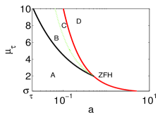
Figure 1: Bifurcation structure of the translating state of the mean field Eqs. (2) for the exponential distribution described in the text ($\sigma_{\tau}=0.2$). The translating state merges with: (i) the stationary state along the continuous red curve $a\mu_{\tau}=1$; and (ii) the circularly rotating state along the dashed black curve $a\langle\tau^{2}\rangle=2$. The component of the translating state parallel to the motion undergoes a Hopf bifurcation along the green, dotted curve. (Color online.)

Equations (2) admit a uniformly translating solution $\mathbf{R}(t)=\mathbf{R}_{0}+\mathbf{V}_{0}\cdot t$ ($\mathbf{R}_{0}$ and $\mathbf{V}_{0}$ are any constant 2D vectors). The speed $|\mathbf{V}_{0}|$ must satisfy

$$|\mathbf{V}_{0}|^{2}=1-a\int_{0}^{\infty}\tau\rho(\tau)d\tau=1-a\mu_{\tau},$$ (3)

which shows that this solution is possible as long as the system parameters lie below the hyperbola $a\mu_{\tau}=1$ in the $(a,\ \mu_{\tau})$ plane. Remarkably, the speed of the of the translating state depends exclusively on the mean of the distribution $\rho(\tau)$ and not on any of the higher moments.

The linear stability of the translating state is examined by taking $X(t)=\sqrt{1-a\mu_{\tau}}\cdot t+\delta X(t)$ and $Y(t)=\delta Y(t)$. The two linearized equations decouple and the stability of motions parallel and perpendicular to the translating direction are determined by the characteristic equations $\mathcal{D}_{\parallel}(\lambda)$ and $\mathcal{D}_{\perp}(\lambda)$, respectively:

$$\mathcal{D}_{\parallel}(\lambda)=\mathcal{F}(\lambda)-(3a\mu_{\tau}-2)\lambda,\quad\mathcal{D}_{\perp}(\lambda)=\mathcal{F}(\lambda)-a\mu_{\tau}\lambda,$$ (4)

where $\mathcal{F}(\lambda)=a\left(1-\langle e^{-\lambda\tau}\rangle\right)+\lambda^{2}$. The function $\langle e^{-\lambda\tau}\rangle$ is the moment generating function of $\rho(\tau)$ since the $n$-th moment is equal to $\langle\tau^{n}\rangle=(-1)^{n}\frac{d^{n}}{d\lambda^{n}}\langle e^{-\lambda\tau}\rangle|_{\lambda=0}$. Regardless of the choice of $a$ and $\rho(\tau)$, the characteristic functions $\mathcal{D}_{\parallel}$ and $\mathcal{D}_{\perp}$ have a zero eigenvalue arising from the translation invariance of Eq. (2) not . There is a fold bifurcation as an eigenvalue of $\mathcal{D}_{\parallel}$ crosses the origin when $a\mu_{\tau}=1$, which marks the disappearance of the translating state as seen from Eq. (3). Numerical analysis Engelborghs (2000) reveals an additional curve on the $(a,\ \mu_{\tau})$ plane (below the curve $a\mu_{\tau}=1$) along which perturbations parallel to the translation undergo a Hopf bifurcation as a complex pair of eigenvalues of $\mathcal{D}_{\parallel}$ cross the imaginary axis.

As for perturbations perpendicular to the translational motion, there is another fold bifurcation as an eigenvalue of $\mathcal{D}_{\perp}$ crosses the origin along the curve $a\langle\tau^{2}\rangle=2$, which represents a bifurcation in which the translating state merges with a circularly rotating state of infinite radius, as discussed below.

Considering a fixed $\sigma_{\tau}$, the overall stability picture of the translating state of Eqs. (2) is as follows (see Fig. 1). For values of $(a,\ \mu_{\tau})$ below the curves $a\langle\tau\rangle=1$ and $a\langle\tau^{2}\rangle=2$ (region A) the translating state is linearly stable . These two curves may cross at a point that we call the ‘zero frequency Hopf point’ (ZFH). The transverse direction of the translating state becomes unstable along the curve $a\langle\tau^{2}\rangle=2$ where this state merges with the circularly rotating state (along the mentioned curve the rotating state has an infinite radius); transverse perturbations of the translating state will thus produce a transition to the rotating state in regions B and C. From the ZFH point, there emanates a Hopf bifurcation curve where the parallel component of the translating state becomes unstable so that in region C there is a transition from the translating state to oscillations along a straight line. Finally, the translating state ceases to exist along the curve $a\langle\tau\rangle=1$ where there is a pitchfork type bifurcation with the stationary steady state solution. The possible behaviors in region D are discussed below.

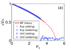
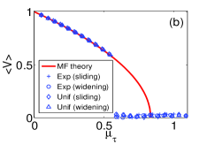
Figure 2: Speed of the translating state of Eqs. (1) and (2) as a function of $\mu_{\tau}$; here $N=150$, $a=0.2$ (a) and $a=1.2$ (b). The red line (color online) represents the mean field result from Eq. (3); the continuous segment marks where the translating state is linearly stable and the dashed segment where it is unstable. The symbols represent numerical simulations of Eqs. (1) for different time delay distributions: sliding exponential and sliding uniform $\sigma_{\tau}$ = 0.5 (a), $\sigma_{\tau}$ = 0.05 (b); widening exponential $\mu_{\tau}=\sigma_{\tau}$ (a) and (b); widening uniform $\mu_{\tau}=\sqrt{3}\sigma_{\tau}$ (a) and (b).

We compare the mean field bifurcation results with the full swarm system via numerical simulations. Here, we make use of two different time delay distributions with mean $\mu_{\tau}$ and standard deviation $\sigma_{\tau}$ to test our findings. The first is an exponential distribution $\rho(\tau)=e^{\frac{\tau-\mu_{\tau}+\sigma_{\tau}}{\sigma_{\tau}}}/\sigma_{\tau}$ for $\tau\geq\mu_{\tau}-\sigma_{\tau}$ and zero otherwise; we require $\sigma_{\tau}\leq\mu_{\tau}$ for proper normalization. The second distribution is a uniform $\rho(\tau)=\frac{1}{2\sqrt{3}\cdot\sigma_{\tau}}$ for $\mu_{\tau}-\sqrt{3}\sigma_{\tau}\leq\tau\leq\mu_{\tau}+\sqrt{3}\sigma_{\tau}$ and zero otherwise; here, we require $\sqrt{3}\sigma_{\tau}\leq\mu_{\tau}$. Moreover, we employ two versions of the mentioned distributions: a ‘sliding’ one ($\sigma_{\tau}$ = const.) and a ‘widening’ version ($\mu_{\tau}\propto\sigma_{\tau}$).

Fig. 2 compares the speed of the swarm obtained from Eq. (3) with the time-averaged speed of the center of mass obtained from simulations (after the decay of transients). The swarm particles are all located at the origin at time zero and move with the speed obtained from Eq. (3) along the $x$ axis. In these simulations, we use both ‘sliding’ ($\sigma_{\tau}$ fixed) and ‘widening’ (both $\mu_{\tau}$ and $\sigma_{\tau}$ vary) versions of the exponential and uniform distributions described above. Fig. 2 shows that the swarm converges to the translating state up to a value of $\mu_{\tau}$ beyond which the swarm converges to a state in which it oscillates back and forth along a line with a near zero time-averaged speed (the average is taken over an interval much longer than the period). The transition to the oscillatory regime occurs earlier than the mean field prediction. The full simulation results show that in this deviation from the mean field, the swarm particles become spread out too far apart and render the approximations leading to Eq. (2) invalid.

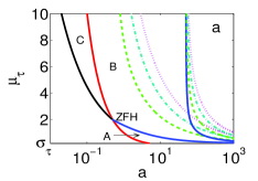
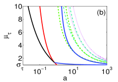
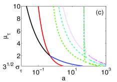
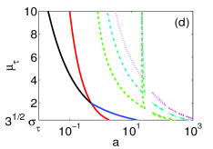
Figure 3: Bifurcation curves of the mean field Eqs. (2) at fixed $\sigma_{\tau}$ for the two time delay distributions $\rho(\tau)$ described in the text: exponential (top) and uniform (bottom). The translational state disappearance curve $a\mu_{\tau}=1$ (red), bifurcation of the translational state with circularly rotating state curve $a\langle\tau^{2}\rangle=2$ (black). The first four members of the stationary state Hopf bifurcation curves are also shown (blue, dashed green, dotted-dashed cyan and dotted magenta). In each panel, $\sigma_{\tau}$ has the value (a) 0.2, (b) 0.95, (c) 0.2 and (d) 0.3, respectively. (Color online.)

In addition to the translating state, Eqs. (2) always possess a stationary state solution $\mathbf{R}(t)=\mathbf{R}_{0}=$ const. In the full system, Eq. (1), the stationary state for the center of mass manifests itself in a swarm ‘ring state’, where some particles rotate clockwise and others counter-clockwise on a circle around a static center of mass. The characteristic equation that governs the linear stability of the stationary state has the form $\big{(}\mathcal{D}(\lambda)\big{)}^{2}=0$, where $\mathcal{D}(\lambda)=\mathcal{F}(\lambda)-\lambda.$ Once more there is a zero eigenvalue for all choices of $a$ and $\rho(\tau)$ that arises from the translation invariance of Eqs. (2). Also, since $\mathcal{D}(0)=0$, $\mathcal{D}^{\prime}(0)=a\mu_{\tau}-1$ and $\lim_{\lambda\rightarrow\infty}\mathcal{D}(\lambda)=\infty$, the condition $a\mu_{\tau}-1<0$ guarantees the existence of at least one real and positive eigenvalue which renders the stationary state linearly unstable. Thus, $a\mu_{\tau}=1$ is a bifurcation curve on the $(a,\mu_{\tau})$ plane along which the uniformly translating state bifurcates with the stationary state.

The stationary state undergoes Hopf bifurcations when the equation $\mathcal{D}(i\omega)=a\left(1-\langle e^{-i\omega\tau}\rangle\right)-\omega^{2}-i\omega=0$ for $\omega\neq 0$ is satisfied. The function $\langle e^{-i\omega\tau}\rangle$ is called the characteristic function of $\rho(\tau)$ and is related to the moment generating function of the distribution; its Taylor series contains all of the moments of $\rho(\tau)$. This shows that the location of the Hopf bifurcations depends on the values of all moments of the time delay distribution. This is in contrast to the region where the translating state exists $a\mu_{\tau}<1$, which involves the first moment only.

At the location of the Hopf bifurcations, circular orbits bifurcate from the stationary state. This may be seen by changing Eq. (2) from the Cartesian $(X,\ Y)$ to polar coordinates $(R,\ \phi)$, noticing that circular orbits $R=R_{0}$, $\phi=\omega t$ are possible as long as

$$\omega^{2}=a\left(1-\langle\cos\omega\tau\rangle\right),\qquad R_{0}=\frac{1}{\omega}\sqrt{1-\frac{a}{\omega}\langle\sin\omega\tau\rangle},$$ (5)

and then realizing that the first of (5) and the condition $R_{0}=0$ are precisely the real and imaginary parts of the Hopf bifurcation conditions $\mathcal{D}(i\omega)=0$.

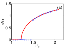
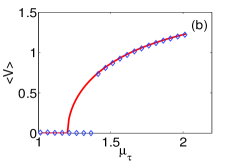
Figure 4: Center of mass speed as a function of $\mu_{\tau}$ for the ‘sliding’ exponential time delay distribution (left) and the ‘sliding’ uniform distribution (right). Here $N=150$, $a=2$. The continuous red curve represents the mean field result from Eq. (5), while the symbols represent the results from numerical simulations of Eqs. (1). (color online)

Generically, the Hopf conditions for the stationary state $\mathcal{D}(i\omega)=0$ yield a family of curves in the $(a,\ \mu_{\tau})$ plane (Fig. 3). The first member of the Hopf family emanates from the crossing of the curves $a\mu_{\tau}=1$ and $a\langle\tau^{2}\rangle=2$; the former curve is where the translating state bifurcates from the stationary state in a pitchfork-like bifurcation. Hence the name ‘Zero Frequency Hopf’ for the Hopf-fold point (Fig. 3a). The first Hopf curve is supercritical and gives rise to a circularly rotating orbit with radius and frequency given by the first solution of Eqs. (5). Below this first Hopf curve and $a\mu_{\tau}=1$, in region A the stationary state is stable. From Eqs. (5) it follows that this circularly rotating orbit collides with the translating state along the curve $a\langle\tau^{2}\rangle=2$ where its radius tends to infinity and its speed to that of the translating state, $\sqrt{1-a\mu_{\tau}}$. Thus, in regions B and C the system converges to the circularly rotating orbit. The different regions change shape for the other panels of Fig. 3, but the dynamics remain as described above.

We compare the mean field prediction for the location of the birth of the circularly rotating state (first Hopf curve) with the full system. Fig. 4 shows the results from numerical simulations of Eqs. (1) at a fixed value of $\sigma_{\tau}$ for increasing $\mu_{\tau}$. We plot the speed of the center of mass averaged over a long time interval, after the decay of transients. In that plot, the near-zero values of the mean speed (in the interval $0\lesssim\mu_{\tau}\lesssim 1.4$) indicate that the particles have converged to the ring state, while for all higher values of $\mu_{\tau}$ the swarm converges to the rotating state. Remarkably, for the highest values of $\mu_{\tau}$, the center of mass of the swarm moves faster than unit speed, the asymptotic speed of uncoupled particles. The reason is that while in its rotating orbit, the mean time-delayed position of the swarm is actually “ahead” of the center of mass at the current time, causing the particles to accelerate forward along the circular orbit.

In summary, we have considered a randomly delay distributed coupled swarm model, and analyzed the bifurcations of various patterns as a function of delay characteristics and coupling strength. In particular, we have shown that the location and shape of the Hopf bifurcation curves is strongly-dependent on all the moments of $\rho(\tau)$. This dependence, in addition to the fact that the succeeding Hopf curves in Fig. 3 exhibit higher frequencies of rotation, makes the higher-order patterns equally sensitive to all the moments of the delay distribution. In the single delay case with distribution $\rho=\delta(\tau-\tau_{0})$, where $\delta(\tau)$ is a Dirac delta function, all of the succeeding Hopf bifurcations are all subcritical and continuous. In contrast, when all moments are present, the bifurcations may not even be continuous, presenting their structure as isolated closed curves bounded by fold bifurcations, as seen in Fig. 3d for a uniform distribution. Finally, we expect that in other globally delay-coupled systems Choi et al. (2000); Marti and Masoller (2003); Kozyreff et al. (2001); Masoller et al. (2009), generic types of behavior involving bifurcations including all moments of the distribution should be present.

The authors gratefully acknowledge the Office of Naval Research for their support. LMR is an NIH post doctoral fellow and BL is a post doctoral fellow of the NRC.

References

- Budrene and Berg (1995) E. Budrene and H. Berg, Nature 376, 49 (1995).
- Toner and Tu (1995) J. Toner and Y. Tu, Phys. Rev. Lett. 75, 4326 (1995).
- Parrish (1999) J. K. Parrish, Science 284, 99 (1999).
- Topaz and Bertozzi (2004) C. Topaz and A. Bertozzi, SIAM Journal on Applied Mathematics 65, 152 (2004).
- Leonard and Fiorelli (2002) N. Leonard and E. Fiorelli, in Proc. of the 40th IEEE Conference on Decision and Control. (2002), vol. 3, pp. 2968–2973.
- Morgan and Schwartz (2005) D. Morgan and I. B. Schwartz, Phys. Lett. A 340, 121 (2005).
- Chuang et al. (2007) Y.-L. Chuang, Y. R. Huang, M. R. D’Orsogna, and A. L. Bertozzi, in Proc. of the 2007 IEEE International Conference on Robotics and Automation. (2007), pp. 2292–2299.
- Lynch et al. (2008) K. M. Lynch, P. Schwartz, I. B. Yang, and R. A. Freeman, IEEE Trans. Robotics 24, 710 (2008).
- Vicsek et al. (1995) T. Vicsek, A. Czirók, E. Ben-Jacob, I. Cohen, and O. Shochet, Phys. Rev. Lett. 75, 1226 (1995).
- Flierl et al. (1999) G. Flierl, D. Grünbaum, S. Levins, and D. Olson, J. Theor. Biol. 196, 397 (1999).
- Toner and Tu (1998) J. Toner and Y. Tu, Phys. Rev. E 58, 4828 (1998).
- Edelstein-Keshet et al. (1998) L. Edelstein-Keshet, J. Watmough, and D. Grunbaum, J. Math. Biol. 36, 515 (1998).
- Erdmann and Ebeling (2005) U. Erdmann and W. Ebeling, Phys. Rev. E 71 (2005).
- Forgoston and Schwartz (2008) E. Forgoston and I. B. Schwartz, Phy. Rev. E 77 (2008), arXiv:0712.2950.
- Aldana et al. (2007) M. Aldana, V. Dossetti, C. Huepe, V. Kenkre, and H. Larralde, Phys. Rev. Lett. 98 (2007).
- Englert et al. (2011) A. Englert, S. Heiligenthal, W. Kinzel, and I. Kanter, Phys. Rev. E 83 (2011).
- Zuo et al. (2010) Z. Zuo, C. Yang, and Y. Wang, Phys. Lett. A 374, 1989 (2010).
- Konishi et al. (2010) K. Konishi, H. Kokame, and N. Hara, Phys. Rev. E 81 (2010).
- Ahlborn and Parlitz (2007) A. Ahlborn and U. Parlitz, Phys. Rev. E 75 (2007).
- Wu et al. (2009) D. Wu, S. Zhu, and X. Luo, EPL 86 (2009).
- Marti et al. (2006) A. C. Marti, M. Ponce C, and C. Masoller, Physica A 371, 104 (2006).
- Omi and Shinomoto (2008) T. Omi and S. Shinomoto, Phys. Rev. E 77 (2008).
- Dykman and Schwartz (2012) M. I. Dykman and I. B. Schwartz (2012), arXiv:1204.6519.
- Mier-y Teran-Romero et al. (2011) L. Mier-y Teran-Romero, E. Forgoston, and I. B. Schwartz (2011), IEEE TRO, accepted. arXiv:1205.0195.
- Lindley et al. (2012) B. Lindley, L. Mier-y Teran, and I. B. Schwartz, ICRA 2012 conference papers, accepted. arXiv:1204.4606. (2012).
- (26) In fact, has a second zero eigenvalue.
- Engelborghs (2000) K. Engelborghs, Tech. Rep. TW-305, Department of Computer Science, K. U. Leuven, Belgium (2000), URL http://www.cs.kuleuven.ac.be/$∼$twr/research/software/de%lay/ddebiftool.shtml.
- Choi et al. (2000) M. Choi, H. Kim, D. Kim, and H. Hong, Phys. Rev. E 61, 371 (2000).
- Marti and Masoller (2003) A. Marti and C. Masoller, Phys. Rev. E 67 (2003).
- Kozyreff et al. (2001) G. Kozyreff, A. Vladimirov, and P. Mandel, Phys. Rev. E 64 (2001).
- Masoller et al. (2009) C. Masoller, M. C. Torrent, and J. Garcia-Ojalvo, Philos. T. Roy. Soc. A 367, 3255 (2009).