Scaling properties of discontinuous maps

Abstract

We study the scaling properties of discontinuous maps by analyzing the average value of the squared action variable $I^{2}$. We focus our study on two dynamical regimes separated by the critical value $K_{c}$ of the control parameter $K$: the slow diffusion ($K<K_{c}$) and the quasilinear diffusion ($K>K_{c}$) regimes. We found that the scaling of $I^{2}$ for discontinuous maps when $K\ll K_{c}$ and $K\gg K_{c}$ obeys the same scaling laws, in the appropriate limits, than Chirikov’s standard map in the regimes of weak and strong nonlinearity, respectively. However, due to absence of KAM tori, we observed in both regimes that $I^{2}\propto nK^{\beta}$ for $n\gg 1$ (being $n$ the $n$-th iteration of the map) with $\beta\approx 5/2$ when $K\ll K_{c}$ and $\beta\approx 2$ for $K\gg K_{c}$.

I Introduction and model

Chirikov’s standard map (CSM), introduced in Ref. C69 , is an area preserving two-dimensional (2D) map for action and angle variables $(I,\theta)$:

$$I_{n+1} = I_{n}+Kf(\theta_{n})\ ,$$

$$\theta_{n+1} = \theta_{n}+I_{n+1}\ ,\quad\mbox{mod}-2\pi\ ,$$ (1)

where $f(\theta_{n})=\sin(\theta_{n})$ (due to this choice of $f(\theta)$, CSM is identified as a continuous map). CSM describes the situation when nonlinear resonances are equidistant in phase space which corresponds to a local description of dynamical chaos licht . Due to this property various dynamical systems and maps can be locally reduced to map (1). Thus, CSM describes the universal and generic behavior of nearly-integrable Hamiltonian systems with two degrees of freedom having a divided phase space composed of stochastic motion bounded by invariant tori (also known as KAM scenario) licht .

CSM develops two dynamical regimes separated by the critical parameter $K_{c}$ C69 ; licht ; C79 ; G79 ; M83 ; MMP84 ; MP85 . When $K<K_{c}$, regime of weak nonlinearity, the motion is mainly regular with regions of stocasticity and $I$ is bounded by KAM surfaces. See for example Fig. 1(a) where we present the Poincaré surface of section for CSM with $K=0.01$. Here, the value of $K$ is so small that the Poincaré surface of section is equivalent to the phase portrait of a one-dimensional pendulum. At $K=K_{c}$, the last KAM curve is destroyed and the transition to global stocasticity takes place. Then, for $K>K_{c}$, regime of strong nonlinearity, $I$ becomes unbounded and increases diffusively. See for example the Poincaré map of Fig. 1(b) where a single trajectory has been iterated $3\times 10^{4}$ times.

Even though CSM describes the universal behavior of area-preserving continuous maps, another class of Hamiltonian dynamical systems is represented by the discontinuous map B98 :

$$I_{n+1} = I_{n}+Kf(\theta_{n})\ ,$$

$$\theta_{n+1} = \theta_{n}+TI_{n+1}\ ,\quad\mbox{mod}-2\pi\ ,$$ (2)

where $f(\theta_{n})=\sin(\theta_{n})\mbox{sgn}[\cos(\theta_{n})]$. Examples of physical systems described by discontinuous maps are 2D billiard models like the stadium billiard stadium1 ; stadium2 and polygonal billiards poly1 ; poly2 . The origin of the discontinuity in map (2) are the sudden translations of the action under the system dynamics.

As well as CSM, map (2) is known to have two different dynamical regimes, however both diffusive, delimited by the critical value $K_{c}=1/T$ B98 . The regimes $K<K_{c}$ and $K>K_{c}$ are known as slow diffusion and quasilinear diffusion regimes, respectively. As an example of the dynamics of map (2), in Fig. 2 we show typical Poincaré surface of sections in both regimes (for comparison purposes we have used the same values of $K$ as in Fig. 1 for CSM). On the one hand, as can be observed by contrasting Figs. 1(a) and 2(a), the main difference between CSM and map (2) is that for $K<K_{c}$ the later does not show regular behavior. In fact, due to the discontinuities of $f(\theta)$ in map (2), KAM theorem is not satisfied and map (2) does not develop the KAM scenario. Since for any $K\neq 0$ the dynamics of map (2) is diffusive, a single trajectory can explore the entire phase space. However, in the slow diffusion regime the dynamics is far from being stochastic due to the sticking of trajectories along cantori (fragments of KAM invariant tori), see Fig. 2(a). On the other hand, for $K>K_{c}$ map (2) shows diffusion similar to that of CSM, compare Figs. 1(b) and 2(b). We want to add that independently of the value of $K\neq 0$, map (2) has five period-one fixed points at $I=0$ and $\theta=[0,\pi/2,\pi,3\pi/2,2\pi]$.

In particular, in Ref. LS07 a scaling analysis of CSM was performed by studying the average value of $I^{2}$ as a function of $K$ and the $n$-th iteration of the map. There, the following scaling law was reported:

$$I^{2}\propto n^{\alpha}K^{\beta}\ ;$$ (3)

where $\alpha\approx 2$ for $K\ll K_{c}$ and small $n$ while $\alpha\approx 1$ for $K\gg K_{c}$ and large $n$, with $\beta\approx 2$ in both cases. The scaling (3) has also been validated for several dynamical systems represented by the standard map such as the Fermi-Ulam model ulam1 ; ulam2 ; ulam3 ; ulam4 ; ulam5 , time-dependent potential wells well , and waveguide billiards ulam5 ; waveguide ; among others other1 ; other2 .

Although map (2) has the same structure than CSM, a systematic investigation of the scaling properties of $I^{2}$ for discontinuous maps is not available in the literature. Thus, in this paper we undertake this task. For this purpose, here we study the properties of the map of Eq. (2) by analyzing the scaling of the average value of the squared action variable $I^{2}$ as a function of $n$, $K$, and $I_{0}$. We choose the scaling approach to $I^{2}$ reported in Ref. LS07 because of the similarity of maps (1) and (2). Moreover, since map (2) shows diffusion in both dynamical regimes ($K<K_{c}$ and $K>K_{c}$), we expect the scaling (3) to be valid for discontinuous maps when diffusion is present with scaling exponents $\alpha$ and $\beta$ to be determined.

Figure 1: Poincaré surface of section for CSM, Eq. (1), with (a) $K=0.01$ and (b) $K=10$. In (a) 20 initial conditions with $\theta_{0}=\pi$ and $I_{0}=[-0.5,0.5)$ were iterated $10^{3}$ times. In (b) a single initial condition with $\theta_{0}=3$ and $I_{0}=0.01$ was iterated $3\times 10^{4}$ times.

Figure 2: Poincaré surface of section for the discontinuous map of Eq. (2) with (a) $K=0.01$ and (b) $K=10$. $T=1$. A single initial condition with $\theta_{0}=3$ and $I_{0}=0.01$ was iterated $3\times 10^{4}$ times.

Figure 3: (a) $I^{2}$ as a function of $n$ in the slow diffusion regime ($K\ll 1$). Full symbols (open symbols) correspond to $I_{0}\ll K$ ($I_{0}\gg K$). Each curve is the average over 1000 trajectories having initial random phases in the interval $0<\theta_{0}<2\pi$. The dashed lines proportional to $n$ and $n^{2}$ are plotted to guide the eye. (b) [(c)] $I^{2}/n^{2}$ [$I^{2}/n$] as a function of $K$ for $n<n_{\mbox{\tiny cr}}^{(1)}$ [$n>n_{\mbox{\tiny cr}}^{(2)}$]. The dashed line equal to $0.17K^{2}$ [$0.17K^{5/2}$] is the best power law-fit to the data.

Figure 4: (a) [(b)] $n_{\mbox{\tiny cr}}^{(1)}$ [$I^{2}_{\mbox{\tiny sat}}$] as a function of $K$. The dashed line equal to $1.1K^{-1/2}$ [$0.31K$] is the best power-law fit to the data. (c) Scaled curves $I^{2}K^{-1}$ as a function of $nK^{1/2}$ in the slow diffusion regime ($K\ll 1$). Full symbols (open symbols) correspond to $I_{0}\ll K$ ($I_{0}\gg K$). Same data as in Fig. 3. The dashed lines show that $I^{2}\propto n^{2}$ for $n<n_{\mbox{\tiny cr}}^{(1)}$ while $I^{2}\propto n$ for $n>n_{\mbox{\tiny cr}}^{(2)}$.

II Results

We compute $I^{2}$ for map (2) following two steps LS07 : First we calculate the average squared action over the orbit associated with the initial condition $j$ as

$$\left<I^{2}_{n,j}\right>=\frac{1}{n+1}\sum^{n}_{i=0}I^{2}_{i,j}\ ,$$

where $i$ refers to the $i$-th iteration of the map. Then, the average value of $I^{2}$ is defined as the average over $M$ independent realizations of the map (by randomly choosing values of $\theta_{0}$):

$$I^{2}(n,K,I_{0})=\frac{1}{M}\sum^{M}_{j=1}\left<I^{2}_{n,j}\right>\ .$$ (4)

In the following, without lost of generality, we set $T=1$.

II.1 Slow diffusion regime

In Fig. 3(a) we present $I^{2}$ as a function of $n$ in the slow diffusion regime ($K\ll 1$) for several combinations of $K$ and $I_{0}$. In fact, $I^{2}$ is always an increasing function of $n$, however its growth is marginal in some iteration intervals producing plateaus in the curves $I^{2}$ vs $n$.

For $I_{0}\ll K$, see full symbols in Fig. 3(a), $I^{2}$ grows up to a crossover iteration number $n_{\mbox{\tiny cr}}^{(1)}$. When $n_{\mbox{\tiny cr}}^{(1)}<n<n_{\mbox{\tiny cr}}^{(2)}$ the trajectories wander around the period-one fixed points of the map making the growth of $I^{2}$ negligible; that is, $I^{2}$ becomes almost constant. We call this constant $I^{2}_{\mbox{\tiny sat}}$. Then, for $n>n_{\mbox{\tiny cr}}^{(2)}$, the trajectories scape from the influence of the period-one fixed points and $I^{2}$ starts to increase again.

In Fig. 3(a) we also explore the case $I_{0}\gg K$, see open symbols. During the first few iteration steps, since $K$ is small as compared to $I_{0}$, $I^{2}$ does not increase significantly as a function of $n$; so, $I^{2}$ remains approximately equal to $I_{0}^{2}$ up to a crossover iteration number $n_{\mbox{\tiny cr}}^{(0)}$. For $n>n_{\mbox{\tiny cr}}^{(0)}$, $I^{2}$ follows the same panorama when increasing $n$ as it does in the case $I_{0}\ll K$: it grows up to $n_{\mbox{\tiny cr}}^{(1)}$, then it becomes approximately equal to $I^{2}_{\mbox{\tiny sat}}$ up to $n_{\mbox{\tiny cr}}^{(2)}$, and finally it grows again.

Then, based on Fig. 3(a), we postulate the following scaling relations:

$$I^{2}(n,K)\propto n^{\alpha}K^{\beta}$$ (5)

for $n<n_{\mbox{\tiny cr}}^{(1)}$ and $n>n_{\mbox{\tiny cr}}^{(2)}$, with

$$n_{\mbox{\tiny cr}}^{(1)}(K)\propto K^{\gamma_{1}}$$ (6)

and

$$n_{\mbox{\tiny cr}}^{(2)}(K)\propto K^{\gamma_{2}}\ ;$$ (7)

in addition

$$I^{2}_{\mbox{\tiny sat}}(K)\propto K^{\delta}\ .$$ (8)

Also, from Fig. 3(a), we concluded that $n_{\mbox{\tiny cr}}^{(0)}=\mbox{const.}\approx 215$. Below, we present a detailed analysis that allows us to obtain the scaling exponents $\alpha$, $\beta$, $\gamma_{1,2}$, and $\delta$.

By performing power-law fittings to the growth regimes of $I^{2}$, we determined that $\alpha\approx 2$ for $n<n_{\mbox{\tiny cr}}^{(1)}$ and $\alpha\approx 1$ when $n>n_{\mbox{\tiny cr}}^{(2)}$. See dashed lines in Fig. 3(a). Once we know the exponents $\alpha$ we can extract the exponents $\beta$. To this end, in Figs. 3(b) and 3(c) we plot $I^{2}/n^{2}$ for $n<n_{\mbox{\tiny cr}}^{(1)}$ and $I^{2}/n$ for $n>n_{\mbox{\tiny cr}}^{(2)}$, respectively, as a function of $K$. The dashed lines, equal to $0.17K^{2}$ and $0.17K^{5/2}$, which are the best power-law fits to the data, prove that $\beta\approx 2$ for $n<n_{\mbox{\tiny cr}}^{(1)}$ and $\beta\approx 5/2$ when $n>n_{\mbox{\tiny cr}}^{(2)}$. In fact, the dependence $I^{2}\propto K^{5/2}$ for $n>n_{\mbox{\tiny cr}}^{(2)}$ is not surprising since theoretical results for the saw-tooth map saw as well as numerical computations on the stadium map stadium1 (both discontinuous maps) show that $I^{2}\propto K^{5/2}$ when $K<K_{c}$ for large $n$. More precisely, for $K<K_{c}$ the dynamics of map (2) is diffusive (after the transient time $n_{\mbox{\tiny cr}}^{(2)}$) with diffusion rate $D=D_{0}K^{5/2}\sqrt{T}$ B98 , where $D=\lim_{n\to\infty}\left<I^{2}(n)\right>/n$ and the average $\left<\cdots\right>$ is performed over an ensemble of trajectories with the same initial action $I_{0}$ and random initial phases $\theta_{0}$. Here, $D_{0}\approx 0.4$ is the constant proper of the choice of $f(\theta)$ we made B98 .

Then, in Figs. 4(a) and 4(b) we show $n_{\mbox{\tiny cr}}^{(1)}$ and $I^{2}_{\mbox{\tiny sat}}$ as a function of $K$, respectively. We computed $n_{\mbox{\tiny cr}}^{(1)}$ as the intersection of a power-law fitting curve $I^{2}\propto n^{2}$ for $n<n_{\mbox{\tiny cr}}^{(1)}$ with the constant curve $I^{2}=I^{2}_{\mbox{\tiny sat}}$. The dashed lines in Figs. 4(a) and 4(b) equal to $1.1K^{-1/2}$ and $0.31K$, respectively, lead to $\gamma_{1}\approx-1/2$ and $\delta\approx 1$. As a consequence of the scalings above, in Fig. 4(c) we present the scaled curves $I^{2}K^{-1}$ as a function of $nK^{1/2}$ showing the collapse of $I^{2}_{\mbox{\tiny sat}}$ and $n_{\mbox{\tiny cr}}^{(1)}$.

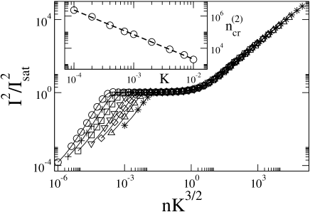
Figure 5: $I^{2}/I^{2}_{\mbox{\tiny sat}}$ as a function of $nK^{3/2}$ in the slow diffusion regime ($K\ll 1$). From left to right: $K=10^{-4}$, $2\times 10^{-4}$, $4\times 10^{-4}$, $10^{-3}$, $2\times 10^{-3}$, $4\times 10^{-3}$, and $10^{-2}$. $I_{0}=K/100$. Inset: $n_{\mbox{\tiny cr}}^{(2)}$ as a function of $K$. The dashed line equal to $1.9K^{-3/2}$ is the best power law-fit to the data.

We want to stress that the scaling of $I^{2}$ for the discontinuous map of Eq. (2) in the slow diffusion regime obeys the same scaling laws than CSM in the regime of weak nonlinearity, see LS07 , except for the appearance of the second crossover iteration number $n_{\mbox{\tiny cr}}^{(2)}$. To study the dependence of $n_{\mbox{\tiny cr}}^{(2)}$ on $K$, in Fig. 5(Inset) we plot $n_{\mbox{\tiny cr}}^{(2)}$ vs $K$. The power-law fitting of the data leads to $\gamma_{2}\approx-3/2$ and a proportionality constant $\approx 1.9$. Then, in the main panel of Fig. 5 we show that the curves $I^{2}/I^{2}_{\mbox{\tiny sat}}$ are properly scaled, for $n>n_{\mbox{\tiny cr}}^{(2)}$, when plotting them as a function of $nK^{3/2}$. The behavior $I^{2}\propto n$ for $n>n_{\mbox{\tiny cr}}^{(2)}$ should be expected in map (2) since here, in contrast to CSM with $K<K_{c}$, the movement is not bounded by KAM tori and particles can diffuse along the phase space cylinder without limit.

Figure 6: (a) $I^{2}$ as a function of $n$ in the quasilinear diffusion regime ($K\gg 1$). Open symbols (full symbols) correspond to $I_{0}\gg K$ ($I_{0}\ll K$). Each curve is the average over 1000 trajectories having initial random phases in the interval $0<\theta_{0}<2\pi$. The dashed lines, plotted to guide the eye, are proportional to $n$. (b) [(c)] $n_{\mbox{\tiny cr}}$ as a function of $I_{0}$ [$K$] for $K=10^{3}$ [$I_{0}=10^{6}$]. The dashed line equal to $3I_{0}^{2}$ [$3.1K^{-2}$] is the best power law-fit to the data.

Figure 7: Scaled curves $I^{2}I_{0}^{-2}$ as a function of $nK^{2}I_{0}^{-2}$ for $I_{0}\gg K$. The dashed line shows that $I^{2}\propto n$ for $n>n_{\mbox{\tiny cr}}$.

II.2 Quasilinear diffusion regime

In Fig. 6(a) we present $I^{2}$ as a function of $n$ in the quasilinear diffusion regime ($K\gg 1$) for several combinations of $K$ and $I_{0}$.

For $I_{0}\ll K$, $I^{2}$ grows proportional to $n$ for all $n$. See full symbols in Fig. 6(a). For $I_{0}\gg K$, $I^{2}$ as a function of $n$ is almost constant and approximately equal to $I_{0}^{2}$ up to a crossover iteration number $n_{\mbox{\tiny cr}}$. Then, when $n>n_{\mbox{\tiny cr}}$, $I^{2}$ increases proportional to $n$. See open symbols in Fig. 6(a). This behavior for $I^{2}$ is completely equivalent to that for CSM in the strong nonlinearity regime LS07 . That is, the scaling given in Eq. (3) is valid for $n>n_{\mbox{\tiny cr}}$ with $\alpha\approx 1$ and $\beta\approx 2$. This is consistent with the random phase approximation C79 that predicts, for $K>K_{c}$, diffusive motion along the $I$ direction with a diffusion rate $D=K^{2}/2$. Moreover, we observed that the crossover iteration number $n_{\mbox{\tiny cr}}$ scales as

$$n_{\mbox{\tiny cr}}(K,I_{0})\propto K^{\gamma_{3}}I_{0}^{\gamma_{4}}\ .$$ (9)

To get the exponents $\gamma_{3,4}$ in the scaling relation above in Figs. 6(b) and 6(c) we plot: (i) $n_{\mbox{\tiny cr}}$ as a function of $I_{0}$ for fixed $K$ and (ii) $n_{\mbox{\tiny cr}}$ as a function of $K$ for fixed $I_{0}$, respectively. Using power-law fittings, see Figs. 6(b) and 6(c), we found that $n_{\mbox{\tiny cr}}\propto K^{-2}I_{0}^{2}$ with a proportionality constant $\approx 3$. Thus, we concluded that $\gamma_{3}\approx-2$ and $\gamma_{4}\approx 2$. Finally, from scaling (9), in Fig. 7 we show that all curves $I^{2}I_{0}^{-2}$ as a function of $nK^{2}I_{0}^{-2}$ colapse into a single one.

III Conclusions

We have studied the scaling properties of the action variable $I$ for the discontinuous map of Eq. (2). We focus on the slow diffusion ($K<K_{c}$) and the quasilinear diffusion ($K>K_{c}$) regimes, being $K_{c}=1/T$. We found that the scaling of $I^{2}$ for map (2) when $K\ll K_{c}$ and $K\gg K_{c}$ obey the same scaling laws than CSM in the regimes of weak and strong nonlinearity LS07 , respectively. Except for that in the slow diffusion regime, due to the absence of KAM tori to bound the motion, $I^{2}\propto n$ for large enough $n$. Also, we conclude that the scaling $I^{2}\propto n^{\alpha}K^{\beta}$ applies to discontinuous maps with

• $\alpha\approx 2$ and $\beta\approx 2$ for $K\ll K_{c}$ and small $n$;

• $\alpha\approx 1$ and $\beta\approx 5/2$ for $K\ll K_{c}$ and large $n$; and

• $\alpha\approx 1$ and $\beta\approx 2$ for $K\gg K_{c}$ and large $n$.

Our results are summarized in Table 1.

	$K\ll 1$	$K\ll 1$	$K\gg 1$	$K\gg 1$
	$I_{0}\ll K$	$I_{0}\gg K$	$I_{0}\ll K$	$I_{0}\gg K$
$I^{2}\approx I^{2}_{0}$	—	$n<n_{\mbox{\tiny cr}}^{(0)}$	—	$n<n_{\mbox{\tiny cr}}$
$I^{2}\propto n^{2}K^{2}$	$n<n_{\mbox{\tiny cr}}^{(1)}$	$n_{\mbox{\tiny cr}}^{(0)}<n<n_{\mbox{\tiny cr}}^{(1)}$	—	—
$I^{2}\approx I^{2}_{\mbox{\tiny sat}}$	$n_{\mbox{\tiny cr}}^{(1)}<n<n_{\mbox{\tiny cr}}^{(2)}$	$n_{\mbox{\tiny cr}}^{(1)}<n<n_{\mbox{\tiny cr}}^{(2)}$	—	—
$I^{2}\propto nK^{5/2}$	$n>n_{\mbox{\tiny cr}}^{(2)}$	$n>n_{\mbox{\tiny cr}}^{(2)}$	—	—
$I^{2}\propto nK^{2}$	—	—	$n>n_{\mbox{\tiny cr}}$	$n>n_{\mbox{\tiny cr}}$

Table 1: Behavior of $I^{2}$ in the slow diffusion ($K\ll 1$) and the quasilinear diffusion ($K\gg 1$) regimes. We have found that $I^{2}_{\mbox{\tiny sat}}\approx 0.31K$, $n_{\mbox{\tiny cr}}^{(0)}\approx 215$, $n_{\mbox{\tiny cr}}^{(1)}\approx 1.1K^{-1/2}$, $n_{\mbox{\tiny cr}}^{(2)}\approx 1.9K^{-3/2}$, and $n_{\mbox{\tiny cr}}\approx 3I_{0}^{2}K^{-2}$.

- (1) B. V. Chirikov, Preprint 267, Institute of Nuclear Physics, Novosibirsk (1969) [Engl. Trans., CERN Trans. 71-40 (1971)].
- (2) A. J. Lichtenberg and M. A. Lieberman, Regular and Chaotic Dynamics (Springer-Verlag, New York, 1992).
- (3) B. V. Chirikov, Phys. Rep. 52, 263 (1979).
- (4) J. M. Greene, J. Math. Phys. 20, 1183 (1979).
- (5) R. S. MacKay, Physica D 7, 283 (1983).
- (6) R. S. MacKay, J. D. Meiss, and I. C. Percival, Physica D 13, 55 (1984).
- (7) R. S. MacKay and I. C. Percival, Comm. Math. Phys. 94, 469 (1985).
- (8) F. Borgonovi, Phys. Rev. Lett. 80, 4653 (1998).
- (9) F. Borgonovi, G. Casati, and B. Li, Phys. Rev. Lett. 77, 4744 (1996).
- (10) G. Casati and T. Prosen, Phys. Rev. E 59, R2516 (1999).
- (11) G. Casati and T. Prosen, Phys. Rev. Lett. 85, 4261 (2000).
- (12) T. Prosen and M. Znidaric, Phys. Rev. Lett. 87, 114101 (2001).
- (13) D. G. Ladeira and J. K. L. Silva, J. Phys. A: Math. Theor. 40, 11467 (2007).
- (14) E. D. Leonel, P. V. E. Mcclintock, and J. K. daSilva, Phys. Rev. Lett. 93, 14101 (2004).
- (15) J. K. L. da Silva, D. G. Ladeira, E. D. Leonel, and P. V. E. Mcclintock, Braz. J. Phys. 36, 700 (2006).
- (16) D. G. Ladeira and J. K. L. da Silva, Phys. Rev. E 73, 026201 (2006).
- (17) E. D. Leonel, J. K. L. da Silva, and S. O. Kamphorst, Physica A 331, 435 (2004).
- (18) E. D. Leonel, in Mathematical Problems in Engineering, vol. 2009, Article ID 367921.
- (19) E. D. Leonel and P. V. E. Mcclintock, J. Phys. A: Math. Gen. 37, 8949 (2004); Chaos 15, 33701 (2005).
- (20) E. D. Leonel, Phys. Rev. Lett. 98, 114102 (2007).
- (21) D. G. Ladeira and J. K. L. da Silva, J. Phys. A: Math. Theor. 41, 365101 (2008).
- (22) J. A. deOliveira, R. A. Bizao, and E. D. Leonel, Phys. Rev. E 81, 046212 (2010).
- (23) I. Dana, N. W. Murray, and I. C. Percival, Phys. Rev. Lett. 62, 233 (1989).