Forbidden minor characterizations for low-rank optimal solutions to semidefinite programs over the elliptope

Abstract

We study a new geometric graph parameter $\text{\rm egd}(G)$, defined as the smallest integer $r\geq 1$ for which any partial symmetric matrix which is completable to a correlation matrix and whose entries are specified at the positions of the edges of $G$, can be completed to a matrix in the convex hull of correlation matrices of ${\rm rank\hskip 1.42262pt}$ at most $r$. This graph parameter is motivated by its relevance to the problem of finding low rank solutions to semidefinite programs over the elliptope, and also by its relevance to the bounded rank Grothendieck constant. Indeed, $\text{\rm egd}(G)\leq r$ if and only if the rank-$r$ Grothendieck constant of $G$ is equal to 1. We show that the parameter $\text{\rm egd}(G)$ is minor monotone, we identify several classes of forbidden minors for $\text{\rm egd}(G)\leq r$ and we give the full characterization for the case $r=2$. We also show an upper bound for $\text{\rm egd}(G)$ in terms of a new tree-width-like parameter ${\rm la_{\boxtimes}}(G)$, defined as the smallest $r$ for which $G$ is a minor of the strong product of a tree and $K_{r}$. We show that, for any 2-connected graph $G\neq K_{3,3}$ on at least 6 nodes, $\text{\rm egd}(G)\leq 2$ if and only if ${\rm la_{\boxtimes}}(G)\leq 2$.

1 Introduction

1.1 Semidefinite programs

A semidefinite program (SDP) is a convex program defined as the minimization of a linear function over an affine section of the cone of positive semidefinite (psd) matrices. Semidefinite programming is a far reaching generalization of linear programing with a wide range of applications in a number of different areas such as approximation algorithms [11], control theory [30], polynomial optimization [20] and quantum information theory [5]. A semidefinite program in canonical primal form looks as follows:

$$\inf\ \langle A_{0},X\rangle$$ (P)

$$\text{subject to }\langle A_{k},X\rangle =b_{k},\qquad k=1,\ldots,m$$

$$X \succeq 0,$$

where $\langle\cdot,\cdot\rangle$ denotes the usual Frobenius inner product of matrices and where $A_{k}\ (0\leq k\leq m)$ are $n$-by-$n$ symmetric matrices, called the coefficient matrices of the SDP. The generalized inequality $X\succeq 0$ means that $X$ is positive semidefinite, i.e., all its eigenvalues are nonnegative.

The field of semidefinite programming has grown enormously in recent years. This success can be attributed to the fact that SDP’s have significant modeling power, exhibit a powerful duality theory and there exist efficient algorithms, both in theory and in practice, for solving them.

The first landmark application of semidefinite programming is the work of Lovász [27] on approximating the Shannon capacity of graphs with the theta number, which gives rise to the only known polynomial time algorithm for calculating these parameters in perfect graphs (see [14]). Starting with the seminal work of Goemans and Williamson on the max-cut problem [12], SDP’s have also proven to be an invaluable tool in the design of approximation algorithms for hard combinatorial optimization problems. This success is vividly illustrated by the fact that many SDP-based approximation algorithms are essentially optimal for a number of problems, assuming the validity of the Unique Games Conjecture (see e.g. [16, 29]).

In this paper we consider the problem of identifying conditions that guarantee the existence of low-rank optimal solutions for a certain class of SDP’s. Results of this type are important for approximation algorithms. Indeed, SDP’s are widely used as convex tractable relaxations for hard combinatorial problems. Then, rank-one solutions typically correspond to optimal solutions of the initial discrete problem and low-rank optimal solutions can decrease the error of the rounding methods and lead to improved performance guarantees.

An illustrative example is the max-cut problem where we are given as input an edge-weighted graph and the goal is to find a cut of maximum weight. It is known that, using the Goemans and Williamson semidefinite programming relaxation, the max-cut problem can be approximated in polynomial time within a factor of 0.878 [12]. Furthermore, assuming that this SDP relaxation for max-cut has an optimal solution of rank 2 (resp., 3), this approximation ratio can be improved to 0.8844 (resp., 0.8818) [2].

Low-rank solutions to SDP’s are also relevant to the study of geometric representations of graphs. In this setting we consider representations obtained by assigning vectors to the vertices of a graph, where we impose restrictions on the vectors labeling adjacent vertices (e.g. orthogonality, or unit distance conditions). Then, questions related to the existence of low-dimensional representations can be reformulated as the problem of deciding the existence of a low-rank solution to an appropriate SDP, and they are connected to interesting graph properties (see [25] for an overview).

1.2 The Gram and extreme Gram dimension parameters

Our main goal in this paper is to identify combinatorial conditions guaranteeing the existence of low-rank optimal solutions to SDP’s. This question has been raised by Lovász in [26]. Quoting Lovász [26, Problem 8.1] it is important to “find combinatorial conditions that guarantee that the semidefinite relaxation has a solution of rank 1”. Furthermore, the version of this problem “with low rank instead of rank 1, also seems very interesting”.

Our focus lies on combinatorial conditions that capture the sparsity of the coefficient matrices of a semidefinite program. To encode this information, with any semidefinite program of the form (P) we associate a graph $\mathcal{A}_{P}=~{}(V_{P},E_{P})$, called the aggregate sparsity pattern of (P), where $V_{P}=\{1,\ldots,n\}$ and $ij\in E_{P}$ if and only if there exists $k\in\{0,1,\ldots,m\}$ such that $(\mathcal{A}_{k})_{ij}\neq~{}0.$

The structure of the aggregate sparsity pattern of a semidefinite program can be used to prove the existence of low-rank optimal solutions. This statement can be formalized by using the following graph parameter, introduced in [22].

Definition 1.1.

[22] The Gram dimension of a graph $G$ is defined as the smallest integer $r\geq 1$ with the following property: Any semidefinite program that attains its optimum and whose aggregate sparsity pattern is a subgraph of $G$ has an optimal solution of rank at most $r$.

It is shown in [22] that the graph parameter $\text{\rm gd}(G)$ is minor monotone. Consequently, by the celebrated graph minor theorem of Robertson and Seymour [31], for any fixed integer $r\geq 1$, the graphs satisfying $\text{\rm gd}(G)\leq r$ can be characterized by a finite list of minimal forbidden minors. The forbidden minors for the graphs with $\text{\rm gd}(G)\leq r$ for the values $r=2,3$ and 4 were identified in [22].

Theorem 1.2.

[22] For any graph $G$ we have that

• $\text{\rm gd}(G)\leq 2\$ if and only if $G$ has no $K_{3}$-minor,

• $\text{\rm gd}(G)\leq 3\$ if and only if $G$ has no $K_{4}$-minor,

• $\text{\rm gd}(G)\leq 4\$ if and only if $G$ has no $K_{5}$ and $K_{2,2,2}$-minors.

Moreover it is shown in [22] that there are close connections between the Gram dimension and results concerning Euclidean graph realizations of Belk and Connelly [3, 4] and with linear algebraic properties of positive semidefinite matrices, whose zero pattern is prescribed by a fixed graph [33].

In this paper we restrict our attention to SDP’s involving only constraints on the diagonal entries, namely, requiring that every feasible matrix has all its diagonal entries equal to 1. Specifically, for a graph $G=([n],E)$ and a vector of edge-weights $w\in{\mathbb{R}}^{E}$, we consider SDP’s of the following form:

$$\text{\rm sdp}(G,w)=\max\sum_{ij\in E}w_{ij}X_{ij}\ \text{ s.t. }\ X_{ii}=1\ (i\in[n]),\ X\succeq 0. P^{w}_{G}$$ ()

Semidefinite programs of this form arise naturally in the context of approximation algorithms. As an example, the Goemans-Williamson SDP relaxation of the max-cut problem (when formulated as a linear program in $\pm 1$ variables) fits into this framework.

Clearly, for any $w\in{\mathbb{R}}^{E}$, the optimal value of ($P^{w}_{G}$) is attained since the objective function is linear and the feasible region is a compact set. Moreover, the aggregate sparsity pattern of ($P^{w}_{G}$) is a subgraph of $G$. Consequently, the semidefinite program ($P^{w}_{G}$) has an optimal solution of rank at most $\text{\rm gd}(G)$ (recall Definition 1.1). Our objective in this paper is to strengthen the upper bound $\text{\rm gd}(G)$. For this we introduce the following graph parameter.

Definition 1.3.

The extreme Gram dimension of a graph $G=([n],E)$, denoted $\text{\rm egd}(G)$, is defined as the smallest integer $r\geq 1$ such that, for any $w\in{\mathbb{R}}^{E}$, the program ($P^{w}_{G}$) has an optimal solution of rank at most $r$.

It follows from the definitions that $\text{\rm egd}(G)$ is upper bounded by $\text{\rm gd}(G)$, i.e.,

$$\text{\rm egd}(G)\leq\text{\rm gd}(G).$$

Moreover, this inequality is strict, for instance, for the complete graph $K_{n}$. Indeed, as we will see in Section 3.2,

$$\text{\rm egd}(K_{n})=\left\lfloor{\sqrt{8n+1}-1\over 2}\right\rfloor<n=\text{\rm gd}(K_{n}),\text{ for }n\geq 2.$$

We will show that the graph parameter $\text{\rm egd}(\cdot)$ is minor monotone (Lemma 3.1). Consequently, by the celebrated graph minor theorem of Robertson and Seymour, for any fixed integer $r\geq 1$, the class of graphs satisfying $\text{\rm egd}(G)\leq r$ can be characterized by a finite list of minimal forbidden minors. It is known that a graph $G$ has $\text{\rm egd}(G)\leq 1$ if and only if $G$ has no $K_{3}$-minor [19]. Our main result in this paper is the characterization of the graphs satisfying $\text{\rm egd}(G)\leq 2$ in terms of two forbidden minors (cf. Theorem 5.1).

Next, we give a series of reformulations for the extreme Gram dimension that will be useful throughout the paper. We start by introducing some necessary definitions and relevant notation. Throughout, ${\mathcal{S}}^{n}$ denotes the set of $n\times n$ symmetric matrices, ${\mathcal{S}}^{n}_{+}$ is the cone of positive semidefinite (psd) matrices and ${\mathcal{S}}^{n}_{++}$ is the cone of positive definite matrices. A psd matrix whose diagonal entries are all equal to one is called a correlation matrix. The set

$$\mathcal{E}_{n}=\{X\in{\mathcal{S}}^{n}_{+}\ :\ X_{ii}=1\ (i\in[n])\}$$

of all $n\times n$ correlation matrices is known as the elliptope. For an integer $r\geq 1$, we define also the (in general non-convex) bounded rank elliptope

$$\mathcal{E}_{n,r}=\{X\in\mathcal{E}_{n}\ :\ {\rm rank\hskip 1.42262pt}X\leq r\}.$$

Given a graph $G=([n],E)$, $\pi_{E}$ denotes the projection from ${\mathcal{S}}^{n}$ onto the subspace ${\mathbb{R}}^{E}$ indexed by the edge set of $G$, i.e.,

$$\pi_{E}:\mathcal{S}^{n}\rightarrow{\mathbb{R}}^{E}\qquad X\mapsto(X_{ij})_{ij\in E}.$$

Lastly, the elliptope of the graph $G=([n],E)$ is defined as the projection of the elliptope $\mathcal{E}_{n}$ onto the subspace indexed by the edge set of $G$:

$$\mathcal{E}(G)=\pi_{E}(\mathcal{E}_{n}).$$

The study of the elliptope is motivated by its relevance to the positive semidefinite matrix completion problem. Indeed, the elements of $\mathcal{E}(G)$ can be seen as the $G$-partial matrices that admit a completion to a full correlation matrix. A $G$-partial matrix is a matrix whose entries are specified only at the off-diagonal positions corresponding to edges of $G$ and at the diagonal positions, with all diagonal entries being equal to 1. Consequently, deciding whether such a $G$-partial matrix admits a positive semidefinite completion is equivalent to deciding membership in the elliptope $\mathcal{E}(G)$.

We now give the first reformulation for the extreme Gram dimension. For a graph $G=([n],E)$ and $w\in{\mathbb{R}}^{E}$, consider the rank-constrained SDP:

$$\text{\rm sdp}_{r}(G,w)=\max\sum_{ij\in E}w_{ij}X_{ij}\ \text{ s.t. }\ X\in\mathcal{E}_{n,r}.$$ (1)

Then, it is clear that $\text{\rm egd}(G)$ can be equivalently defined as the smallest integer $r\geq 1$ for which equality holds:

$$\text{\rm sdp}(G,w)=\text{\rm sdp}_{r}(G,w),\ \text{ for all }w\in{\mathbb{R}}^{E}.$$ (2)

For the second reformulation of the parameter $\text{\rm egd}(\cdot)$, we first observe that program ($P^{w}_{G}$) is equivalent to

$$\text{\rm sdp}(G,w)=\max\ w^{\sf T}x\ \text{ s.t. }\ x\in\mathcal{E}(G),$$ (3)

and thus it corresponds to optimization over the projected elliptope $\mathcal{E}(G)$. On the other hand, as its objective function is linear, the (non-convex rank constrained) program (1) can be equivalently reformulated as optimization over the convex set $\pi_{E}(\text{\rm conv}(\mathcal{E}_{n,r})$). That is,

$$\text{\rm sdp}_{r}(G,w)=\max\ w^{\sf T}x\ \text{ s.t. }\ x\in\pi_{E}(\text{\rm conv}(\mathcal{E}_{n,r})).$$ (4)

Then, in view of (2), we arrive at the following geometric reformulation for $\text{\rm egd}(\cdot)$.

Lemma 1.4.

The extreme Gram dimension of a graph $G=([n],E)$ is equal to the smallest integer $r\geq 1$ for which

$$\mathcal{E}(G)=\pi_{E}(\text{\rm conv}(\mathcal{E}_{n,r})).$$ (5)

Using this geometric reformulation for the parameter $\text{\rm egd}(\cdot)$, we are now in a position to explain why we have chosen to name it as the extreme Gram dimension. Since the inclusion $\pi_{E}(\text{\rm conv}(\mathcal{E}_{n,r}))\subseteq\mathcal{E}(G)$ is always valid, it follows from Lemma 1.4 that $\text{\rm egd}(G)$ is equal to the smallest $r\geq 1$ for which the reverse inclusion $\mathcal{E}(G)\subseteq\pi_{E}(\text{\rm conv}(\mathcal{E}_{n,r}))$ holds. Moreover, since $\mathcal{E}(G)$ is a compact convex subset of ${\mathbb{R}}^{E}$, by the Krein–Milman theorem, $\mathcal{E}(G)$ is equal to the convex hull of its set of extreme points. With ${\rm ext\hskip 1.42262pt}\mathcal{E}(G)$ denoting the set of extreme points of $\mathcal{E}(G)$, it follows that

$$\mathcal{E}(G)\subseteq\pi_{E}(\text{\rm conv}(\mathcal{E}_{n,r}))\Longleftrightarrow{\rm ext\hskip 1.42262pt}\mathcal{E}(G)\subseteq\pi_{E}(\mathcal{E}_{n,r}).$$

Summarizing, the parameter $\text{\rm egd}(G)$ can be reformulated as the smallest integer $r\geq 1$ for which:

$${\rm ext\hskip 1.42262pt}\mathcal{E}(G)\subseteq\pi_{E}(\mathcal{E}_{n,r}).$$ (6)

In other words, $\text{\rm egd}(G)$ is equal to the smallest $r\geq 1$ for which every extreme point of $\mathcal{E}(G)$ has a positive semidefinite completion of rank at most $r$.

1.3 Relation with the Gram dimension

As we will now see, both $\text{\rm gd}(\cdot)$ and $\text{\rm egd}(\cdot)$ can be phrased within the common framework of Gram representations introduced below. This reformulation will allow us to clarify the relationship between these two parameters.

Definition 1.5.

Given a graph $G=([n],E)$ and a vector $x\in{\mathbb{R}}^{E}$, a Gram representation of $x$ in ${\mathbb{R}}^{r}$ is a set of unit vectors $p_{1},\ldots,p_{n}\in{\mathbb{R}}^{r}$ such that

$$x_{ij}=p_{i}^{\sf T}p_{j}\ \ \forall\{i,j\}\in E.$$

The Gram dimension of $x\in\mathcal{E}(G)$, denoted by $\text{\rm gd}(G,x)$, is the smallest integer $r\geq 1$ for which $x$ has such a Gram representation in ${\mathbb{R}}^{r}$.

Recall that, for a matrix $X\in\mathcal{S}^{n}$, $X\in\mathcal{E}_{n}$ if and only if there exists a family of unit vectors $p_{1},\ldots,p_{n}$ such that $X_{ij}=p_{i}^{\sf T}p_{j}$ for all $i,j\in[n]$. Hence, for a vector $x\in\mathcal{E}(G)$, it is easy to see that $\text{\rm gd}(G,x)$ is equal to the smallest rank of a completion for $x$ to a full correlation matrix.

Using this notion of Gram representations, we find the following equivalent definition for the Gram dimension of a graph, as originally introduced in [22]. We sketch a proof of this fact for clarity.

Lemma 1.6.

For any graph $G=(V,E)$,

$$\text{\rm gd}(G)=\max_{x\in\mathcal{E}(G)}\text{\rm gd}(G,x).$$ (7)

Proof.

Let $x\in\mathcal{E}(G)$. Then $\text{\rm gd}(G,x)$ is the smallest $r$ for which the SDP:

$$\min\ 0\ \text{ s.t. }X\in\mathcal{E}_{n},\ X_{ij}=x_{ij}\ \forall ij\in E$$

has an optimal solution of rank at most $r$. As the aggregate sparsity pattern of this SDP is equal to $G$, it follows that $\text{\rm gd}(G)\geq\text{\rm gd}(G,x)$. This shows the inequality $\text{\rm gd}(G)\geq\max_{x\in\mathcal{E}(G)}\text{\rm gd}(G,x)$. We now show the reverse inequality: $\text{\rm gd}(G)\leq\max_{x\in\mathcal{E}(G)}\text{\rm gd}(G,x)=:r.$ For this consider an SDP of the form (P) whose aggregate sparsity pattern is a subgraph of $G$. Let $X$ be an optimal solution of (P); we construct another optimal solution $X^{\prime}$ with rank at most $r$. For simplicity let us assume that all diagonal entries of $X$ are positive (if not, just work with the principal submatrix of $X$ with only positive diagonal entries). With $D$ denoting the diagonal matrix with diagonal entries $\sqrt{X_{ii}}$, we can rescale $X$ so that $Y:=D^{-1}XD^{-1}$ belongs to $\mathcal{E}_{n}$. Then, the projection $y=\pi_{E}(Y)$ belongs to $\mathcal{E}(G)$. Hence there exists a matrix $Y^{\prime}\in\mathcal{E}_{n}$ of rank at most $r$ such that $\pi_{E}(Y^{\prime})=y$. Scaling back, the matrix $X^{\prime}=DY^{\prime}D$ is a psd completion of $x$ and thus it is also an optimal solution of (P). Moreover, $X^{\prime}$ has rank at most $r$, which concludes the proof. ∎

Moreover, we have the following analogous reformulation for the extreme Gram dimension.

Lemma 1.7.

For any graph $G$,

$$\text{\rm egd}(G)=\max_{x\in{\rm ext\hskip 1.42262pt}\mathcal{E}(G)}\text{\rm gd}(G,x).$$ (8)

Proof.

Let $x\in{\rm ext\hskip 1.42262pt}\mathcal{E}(G)$. By (6), $x$ has a psd completion of rank at most $\text{\rm egd}(G)$ and thus $\text{\rm gd}(G,x)\leq\text{\rm egd}(G)$. This shows $\max_{x\in{\rm ext\hskip 1.42262pt}\mathcal{E}(G)}\text{\rm gd}(G,x)\leq\text{\rm egd}(G)$. The reverse inequality follows directly from (6). ∎

Combining (7) and (8) we find again the inequality: $\text{\rm egd}(G)\leq\text{\rm gd}(G)$.

1.4 Relation with the bounded rank Grothendieck constant

The study of programs of the form (1) is of significant practical interest, the main motivation coming from statistical mechanics and in particular from the $r$-vector model introduced by Stanley [32]. This model consists of an interaction graph $G=(V,E)$, where vertices correspond to particles and edges indicate whether there is interaction (ferromagnetic or antiferromagnetic) between the corresponding pair of particles. Additionally, there is a potential function $A:~{}V\times V\rightarrow{\mathbb{R}}$ satisfying $A_{ij}=0$ if $ij\not\in E$, $A_{ij}>0$ if there is ferromagnetic interaction between $i$ and $j$ and $A_{ij}<0$ if there is antiferromagnetic interaction between $i$ and $j$. Additionally, particles possess a vector valued spin given by a function $f:V\rightarrow\mathbb{S}^{r-1}$, where $\mathbb{S}^{r-1}$ denotes the unit sphere in ${\mathbb{R}}^{r}$. Assuming that there is no external field acting on the system, its total energy is given by the Hamiltonian defined as

$$H(f)=-\sum_{ij\in E}A_{ij}f(i)^{\sf T}f(j).$$

A ground state is a configuration of spins that minimizes the Hamiltonian. The case $r=1$ corresponds to the Ising model, the case $r=2$ corresponds to the XY model and the case $r=3$ to the Heisenberg model. Consequently, calculating the Hamiltonian and computing ground states in any of these models amounts to solving a rank-constrained semidefinite program of the form (1).

As the rank function is non-convex and non-differentiable, such problems are computationally challenging. Indeed, problem (1) (or its reformulation (4)) is hard. In the case $r=1$, the feasible region of (4) is equal to the cut polytope of the graph $G$ (in $\pm 1$ variables) and thus (4) is $\mathsf{NP}$-hard. It is believed that (1) is also $\mathsf{NP}$-hard for any fixed integer $r\geq 2$ (cf., e.g., the quote of Lovász [28, p. 61]). For any $r\geq 2$, it is shown in [10] that membership in $\pi_{E}(\text{\rm conv}(\mathcal{E}_{n,r}))$ is $\mathsf{NP}$-hard. This motivates the need for identifying tractable instances for (1).

Clearly ($P^{w}_{G}$) is a semidefinite programming relaxation for program (1) obtained by removing the rank constraint. The quality of this relaxation is measured by its integrality gap defined below.

Definition 1.8.

The rank-$r$ Grothendieck constant of a graph $G$, denoted as $\kappa(r,G)$, is defined as

$$\kappa(r,G)=\sup_{w\in{\mathbb{R}}^{E}}\frac{\text{\rm sdp}(G,w)}{\text{\rm sdp}_{r}(G,w)}.$$ (9)

For $r=1$, the special case where $G$ is a complete bipartite graph was studied by A. Grothendieck [13], although in a quite different language, and for general graphs by Alon et al. [1]. The general case $r\geq 2$ is studied by Briët et al. [6], their main motivation being the polynomial-time approximation of ground states of spin glasses.

The extreme Gram dimension of a graph is closely related to the rank-r Grothendieck constant of a graph as we now point out. Indeed it follows directly from the definitions that a graph has extreme Gram dimension at most $r$ if and only if its rank-$r$ Grothendieck constant is 1, i.e.,

$$\text{\rm egd}(G)\leq r\Longleftrightarrow\kappa(r,G)=1.$$

Hence, for any graph $G$ with $\text{\rm egd}(G)\leq r$, we have that $\text{\rm sdp}(G,w)=\text{\rm sdp}_{r}(G,w)$ for all $w\in{\mathbb{R}}^{E}$, and thus the value of program (1) can be approximated within arbitrary precision in polynomial time.

1.5 Contributions and outline of the paper

We now briefly summarize the main contributions of the paper. Our first result is to show that the new graph parameter $\text{\rm egd}(G)$ is minor monotone. As a consequence the class ${\mathcal{G}}_{r}$ consisting of all graphs $G$ with $\text{\rm egd}(G)\leq r$ can be characterized by finitely many minimal forbidden minors. It is known that for the case $r=1$ the only forbidden minor is $K_{3}$, i.e., the class ${\mathcal{G}}_{1}$ consists of all forests [19]. One of the main contributions of this paper is a complete characterization of the class ${\mathcal{G}}_{2}$ (Theorem 5.2).

Furthermore, we identify three families of graphs $F_{r},G_{r}$, $H_{r}$ which are forbidden minors for the class ${\mathcal{G}}_{r-1}$. This gives all the minimal forbidden minors for $r\leq 2$. The graphs $G_{r}$ were already considered in [7, 18].

On the other hand we show an upper bound for the extreme Gram dimension in terms of a tree-width-like parameter. This graph parameter, which we denote as ${\rm la_{\boxtimes}}(G)$, is defined as the smallest integer $r$ for which $G$ is a minor of the strong product $T\boxtimes K_{r}$ of a tree $T$ and the complete graph $K_{r}$. We call it the strong largeur d’arborescence of $G$, in analogy with the largeur d’arborescence ${\rm la_{\square}}(G)$ introduced by Colin de Verdière [7], defined similarly by replacing the strong product with the Cartesian product of graphs. Another main contribution is to show the upper bound: $\text{\rm egd}(G)\leq{\rm la_{\boxtimes}}(G)$.

Our main result is that, for a graph $G\neq K_{3,3}$ which is 2-connected and has at least 6 nodes, $\text{\rm egd}(G)\leq 2$ if and only if ${\rm la_{\boxtimes}}(G)\leq 2$ if and only if $G$ does not have $F_{3}$ or $H_{3}$ as a minor. We also characterize the graphs with ${\rm la_{\boxtimes}}(G)\leq 2$ and recover the characterization of [17] for the graphs with ${\rm la_{\square}}(G)\leq 2$.

The results and techniques in the paper come in two flavours: in Section 4 they rely mostly on the geometry of faces of the elliptope and linear algebraic tools to construct suitable extreme points of the projected elliptope and, in Section 5, they are purely graph theoretic.

The paper is organized as follows. Section 2 contains preliminaries about graphs and basic facts about the geometry of the faces of the elliptope. In Section 3 we study properties of the new graph parameter $\text{\rm egd}(G)$. In particular, in Section 3.1 we show minor-monotonicity and investigate the behaviour under the clique-sum graph operation and in Section 3.2 we show some bounds on $\text{\rm egd}(G)$. In Section 3.3 we introduce the strong largeur d’arborescence parameter ${\rm la_{\boxtimes}}(G)$ and we show that it upper bounds the extreme Gram dimension, i.e., that $\text{\rm egd}(G)\leq{\rm la_{\boxtimes}}(G)$. In Sections 4.1-4.3 we compute the extreme Gram dimension of the three graph classes $F_{r}$, $G_{r}$ and $H_{r}$ and in Section 4.4 we compute the extreme Gram dimension of the graphs $K_{5}$ and $K_{3,3}$, which play a special role within the class ${\mathcal{G}}_{2}$. Section 5 is devoted to identifying the forbidden minors for the class ${\mathcal{G}}_{2}$. In Section 5.1 we characterize the chordal graphs in ${\mathcal{G}}_{2}$ (Theorem 5.4). In Section 5.2 we show that any graph with no minor $F_{3}$ or $K_{4}$ admits a chordal extension avoiding these two minors (Theorem 5.7) and in Section 5.3 we show the analogous result for graphs with no $F_{3}$ and $H_{3}$ minor (Theorem 5.12). Finally in Section 6 we characterize the graphs with ${\rm la_{\boxtimes}}(G)\leq 2$, we explain the links to results about ${\rm la_{\square}}(G)$, and we point out connections with the graph parameter $\nu(G)$ of Colin de Verdière [7].

2 Preliminaries

2.1 Preliminaries about graphs

We recall some definitions about graphs. Let $G=(V,E)$ be a graph, we also denote its node set by $V(G)$ and its edge set by $E(G)$. A component is a maximal connected subgraph of $G$. A cutset is a set $U\subseteq V$ for which $G\backslash U$ (deleting the nodes in $U$) has more connected components than $G$, $U$ is a cut node if $|U|=1$, and $G$ is 2-connected if it is connected and has no cut node. For $W\subseteq V$, $G[W]$ is the subgraph induced by $W$. Given $\{u,v\}\not\in E(G)$, $G+\{u,v\}$ is the graph obtained by adding the edge $\{u,v\}$ to $G$.

Given an edge $e=\{u,v\}\in E$, $G\backslash e=(V,E\setminus\{e\})$ is the graph obtained from $G$ by deleting the edge $e$ and $G/e$ is obtained by contracting the edge $e$: Replace the two nodes $u$ and $v$ by a new node, adjacent to all the neighbors of $u$ and $v$. A graph $M$ is a minor of $G$, denoted as $M\preceq G$, if $M$ can be obtained from $G$ by a series of edge deletions and contractions and node deletions. Equivalently, $M$ is a minor of a connected graph $G$ if there is a partition of $V(G)$ into nonempty subsets $\{V_{i}:i\in V(M)\}$ where each $G[V_{i}]$ is connected and, for each edge $\{i,j\}\in E(M)$, there exists at least one edge in $G$ between $V_{i}$ and $V_{j}$. The collection $\{V_{i}:i\in V(M)\}$ is called an $M$-partition of $G$ and the $V_{i}$’s are the classes of the partition.

Given a finite list ${\mathcal{M}}$ of graphs, ${\mathcal{F}}({\mathcal{M}})$ denotes the collection of all graphs that do not admit any graph in ${\mathcal{M}}$ as a minor. By the celebrated graph minor theorem of Robertson and Seymour [31], any family of graphs which is closed under the operation of taking minors is of the form ${\mathcal{F}}({\mathcal{M}})$ for some finite set ${\mathcal{M}}$ of graphs. In this setting, closed means that every minor of a graph in the family is also contained in the family.

A graph parameter is any function from the set of graphs (up to isomorphism) to the natural numbers. A graph parameter $f(\cdot)$ is called minor monotone if

$$f(G\backslash e)\leq f(G)\text{ and }f(G/e)\leq f(G),$$

for any graph $G$ and any edge $e$ of $G$. Given a minor monotone graph parameter $f(\cdot)$ and a fixed integer $k\geq 1$, the family of graphs $G$ satisfying $f(G)\leq k$ is closed under taking minors. Then, for any fixed integer $k\geq 1$ there exists a forbidden minor characterization for the family of graphs satisfying $f(G)\leq k$.

A homeomorph (or subdivision) of a graph $M$ is obtained by replacing its edges by paths. When $M$ has maximum degree at most 3, $G$ admits $M$ as a minor if and only if it contains a homeomorph of $M$ as a subgraph.

A clique in $G$ is a set of pairwise adjacent nodes and $\omega(G)$ denotes the maximum cardinality of a clique in $G$. A $k$-clique is a clique of cardinality $k$.

Let $G_{1}=(V_{1},E_{1})$, $G_{2}=(V_{2},E_{2})$ be two graphs, where $V_{1}\cap V_{2}$ is a clique in both $G_{1}$ and $G_{2}$. Their clique sum is the graph $G=(V_{1}\cup V_{2},E_{1}\cup E_{2})$, also called their clique $k$-sum when $k=|V_{1}\cap V_{2}|$.

If $C$ is a circuit in $G$, a chord of $C$ is an edge $\{u,v\}\in E$ where $u$ and $v$ are two nodes of $C$ that are not consecutive on $C$. $G$ is said to be chordal if every circuit of length at least 4 has a chord. As is well known, a graph $G$ is chordal if and only if $G$ is a clique sum of cliques.

The Cartesian product of two graphs $G=(V,E)$ and $G^{\prime}=(V^{\prime},E^{\prime})$, denoted by $G\square G^{\prime}$, is the graph with node set $V\times V^{\prime}$, where distinct nodes $(i,i^{\prime}),(j,j^{\prime})\in V\times V^{\prime}$ are adjacent in $G\square G^{\prime}$ when $i=j$ and $(i^{\prime},j^{\prime})\in G^{\prime}$, or $(i,j)\in G$ and $i^{\prime}=j^{\prime}$.

The strong product of two graphs $G=(V,E)$ and $G^{\prime}=(V^{\prime},E^{\prime})$, denoted by $G\boxtimes G^{\prime}$, is the graph with node set $V\times V^{\prime}$, where distinct nodes $(i,i^{\prime}),(j,j^{\prime})\in V\times V^{\prime}$ are adjacent in $G\boxtimes G^{\prime}$ when $i=j$ or $(i,j)\in E$, and $i^{\prime}=j^{\prime}$ or $(i^{\prime},j^{\prime})\in E^{\prime}$.

The treewidth of a graph $G$, denoted by ${\rm tw}(G)$, is the smallest integer $k\geq 1$ such that $G$ is contained in a clique sum of copies of $K_{k+1}$. This parameter was introduced by Robertson and Seymour in their fundamental work on graph minors [31] and is commonly used in the parameterized complexity analysis of graph algorithms. It is known that ${\rm tw}(\cdot)$ is a minor-monotone graph parameter and that ${\rm tw}(K_{n})=n-1$ (see e.g. [9]). It follows from the above definition that, if $G$ is obtained as the clique sum of $G_{1}$ and $G_{2}$ then

$${\rm tw}(G)=\max\{{\rm tw}(G_{1}),{\rm tw}(G_{2})\}.$$ (10)

Colin de Verdière [7] introduced the following treewidth-like parameter: The largeur d’arborescence of a graph $G$, denoted by ${\rm la_{\square}}(G)$, is the smallest integer $r\geq 1$ for which $G$ is a minor of $T\Box K_{r}$ for some tree T. Then,

$${\rm tw}(G)\leq{\rm la_{\square}}(G)\leq{\rm tw}(G)+1,$$

where the upper bound is shown in [7] and the lower bound in [33].

The strong largeur d’arborescence of a graph $G$, denoted by ${\rm la_{\boxtimes}}(G)$, is the smallest integer $r\geq 1$ for which $G$ is a minor of $T\boxtimes K_{r}$ for some tree T. In Section 3.3 we will come back to this parameter and we will show that it is an upper bound for the extreme Gram dimension.

2.2 Preliminaries about positive semidefinite matrices

Throughout we set $[n]=\{1,\dots,n\}$. For $U\subseteq[n]$ and $X\in{\mathcal{S}}^{n}$, $X[U]$ denotes the principal submatrix of $X$ with row and column indices in $U$ and, for $j\in[n]$, $X[\cdot,j]$ denotes the $j$-th column of $X$. For a set $A\subseteq{\mathbb{R}}^{n}$, $\langle A\rangle$ denotes the vector space spanned by $A$ and $\text{\rm conv}A$ denotes the convex hull of $A$.

We group here some basic properties of positive semidefinite matrices that we will use throughout. Given vectors $p_{1},\ldots,p_{n}\in{\mathbb{R}}^{k}$ ($k\geq 1$), we let the matrix ${\rm Gram}(p_{1},\ldots,p_{n})=(p_{i}^{\sf T}p_{j})_{i,j=1}^{n}$ denote their Gram matrix. Then, the rank of ${\rm Gram}(p_{1},\ldots,p_{n})$ is equal to $\dim\langle p_{1},\ldots,p_{n}\rangle$. If $X={\rm Gram}(p_{1},\ldots,p_{n})$ we also say that the $p_{i}$’s form a Gram representation of $X$. As is well known, a matrix $X\in{\mathcal{S}}^{n}$ is positive semidefinite if and only if

$$\exists p_{1},\ldots,p_{n}\in{\mathbb{R}}^{k}\text{ for some }k\geq 1\text{ such that }X={\rm Gram}(p_{1},\ldots,p_{n}).$$ (11)

For $X\in{\mathcal{S}}^{n}$, ${\rm Ker\hskip 1.42262pt}X$ is the kernel of $X$, consisting of the vectors $u\in{\mathbb{R}}^{n}$ such that $Xu=0$. When $X\succeq 0$, $u\in{\rm Ker\hskip 1.42262pt}X$ (i.e., $Xu=0$) if and only if $u^{T}Xu=0$. Given a matrix $X\in{\mathcal{S}}^{n}$ in block-form

$$X=\left(\begin{matrix}A&B^{T}\cr B&C\end{matrix}\right),$$

the following holds:

$$\text{if }X\succeq 0,\text{ then }{\rm Ker\hskip 1.42262pt}A\subseteq{\rm Ker\hskip 1.42262pt}B.$$ (12)

2.3 The geometry of the elliptope

In this section we group some geometric properties of the elliptope, which we will need in the paper. First we recall some basic definitions and facts about faces of convex sets.

Given a convex set $K$, a set $F\subseteq K$ is a face of $K$ if, for all $x\in F$, the condition $x=ty+(1-t)z$ with $y,z\in K$ and $t\in(0,1)$ implies $y,z\in F$. For $x\in K$ the smallest face $F(x)$ of $K$ containing $x$ is well defined, it is the unique face of $K$ containing $x$ in its relative interior. A point $x\in K$ is an extreme point of $K$ if $F(x)=\{x\}.$ We denote the set of extreme points of a convex set $K$ by ${\rm ext\hskip 1.42262pt}K$. A useful property of extreme points is that if $F$ is a face of the convex set $K$ then

$${\rm ext\hskip 1.42262pt}F\subseteq{\rm ext\hskip 1.42262pt}K.$$ (13)

Moreover, $z$ is said to be a perturbation of $x\in K$ if $x\pm\epsilon z\in K$ for some $\epsilon>0$, then the segment $[x-\epsilon z,x+\epsilon z]$ is contained in $F(x)$ and the dimension of $F(x)$ is equal to the dimension of the linear space ${\mathcal{P}}(x)$ of perturbations of $x$.

We now recall some facts about the faces of the elliptope that we need here. We refer e.g. to [21] for details. For a matrix $X\in\mathcal{E}_{n}$, the smallest face ${F}(X)$ of $\mathcal{E}_{n}$ containing $X$ is given by

$${F}(X)=\{Y\in\mathcal{E}_{n}:{\rm Ker\hskip 1.42262pt}X\subseteq{\rm Ker\hskip 1.42262pt}Y\}.$$ (14)

Therefore, two matrices in the relative interior of a face $F$ of $\mathcal{E}_{n}$ have the same rank, while ${\rm rank\hskip 1.42262pt}X>{\rm rank\hskip 1.42262pt}Y$ if $X$ is in the relative interior of $F$ and $Y$ lies on the boundary of $F$. Here is the explicit description of the space ${\mathcal{P}}(X)$ of perturbations of a matrix $X\in\mathcal{E}_{n}$.

Proposition 2.1.

([24], see also [8, §31.5]) Let $X\in\mathcal{E}_{n}$ with rank $r$. Let $u_{1},\ldots,u_{n}\in{\mathbb{R}}^{r}$ be a Gram representation of $X$, let $U$ be the $r\times n$ matrix with columns $u_{1},\ldots,u_{n}$ and set ${\mathcal{U}}_{V}=\langle u_{1}u_{1}^{\sf T},\ldots,u_{n}u_{n}^{\sf T}\rangle\subseteq{\mathcal{S}}^{r}.$ The space of perturbations ${\mathcal{P}}(X)$ at $X$ is given by

$${\mathcal{P}}(X)=U^{\sf T}{\mathcal{U}}_{V}^{\perp}U=\{U^{\sf T}RU:R\in{\mathcal{S}}^{r},\langle R,u_{i}u_{i}^{\sf T}\rangle=0\ \forall i\in[n]\}$$ (15)

and the dimension of the smallest face ${F}(X)$ of $\mathcal{E}_{n}$ containing $X$ is

$$\dim{F}(X)=\dim{\mathcal{P}}(X)={r+1\choose 2}-\dim\ {\mathcal{U}}_{V}.$$ (16)

In particular, $X$ is an extreme point of $\mathcal{E}_{n}$ if and only if

$${r+1\choose 2}=\dim\ {\mathcal{U}}_{V}.$$ (17)

Hence, if $X\in{\rm ext\hskip 1.42262pt}\mathcal{E}_{n}$ with ${\rm rank\hskip 1.42262pt}X=r$ then

$${r+1\choose 2}\leq n.$$ (18)

An application for the previous proposition is the following example:

Example 2.1.

Let $e_{1},\dots,e_{r}\in{\mathbb{R}}^{r}$ be the standard unit vectors. The matrix with Gram representation $\{e_{i}:\,i\in[r]\}\cup\{(e_{i}+e_{j})/\sqrt{2}:\,1\leq i<j\leq r\}$ is an extreme point of $\mathcal{E}_{n}$, since ${\mathcal{U}}_{V}$ is full dimensional in ${\mathcal{S}}^{r}$, where $n=\binom{r+1}{2}$.

The next theorem shows that every number in the range prescribed in (18) corresponds to an extremal element of $\mathcal{E}_{n}$.

Theorem 2.2.

[24] For any natural number $r$ satisfying $\binom{r+1}{2}\leq n$ there exists a matrix $X\in\mathcal{E}_{n}$ which is an extreme point of $\mathcal{E}_{n}$ and has rank equal to $r$.

Next we establish some tools which will be useful to study the extreme points of the projected elliptope $\mathcal{E}(G)$.

Lemma 2.3.

Consider a partial matrix $x\in\mathcal{E}(G)$ and let $X\in\mathcal{E}_{n}$ be a rank $r$ completion of $x$ with Gram representation $\{u_{1},\ldots,u_{n}\}$ in ${\mathbb{R}}^{r}$. Moreover, let $U$ be the $r\times n$ matrix with columns $u_{1},\ldots,u_{n}$. Set

$$U_{ij}={u_{i}u_{j}^{\sf T}+u_{j}u_{i}^{\sf T}\over 2},\ {\mathcal{U}}_{V}=\langle U_{ii}:i\in V\rangle,\ {\mathcal{U}}_{E}=\langle U_{ij}:\{i,j\}\in E\rangle\subseteq{\mathcal{S}}^{r}.$$ (19)

If $x$ is an extreme point of $\mathcal{E}(G)$, then ${\mathcal{U}}_{E}\subseteq{\mathcal{U}}_{V}$.

Proof.

Assume that ${\mathcal{U}}_{E}\not\subseteq{\mathcal{U}}_{V}$. Then there exists a matrix $R\in{\mathcal{U}}_{V}^{\perp}\setminus{\mathcal{U}}_{E}^{\perp}$. As $R\in{\mathcal{U}}_{V}^{\perp}$, the matrix $Z=U^{\sf T}RU=(\langle R,U_{ij}\rangle)_{i,j=1}^{n}\in{\mathcal{S}}^{n}$ is a perturbation of $X$ (recall (15) and (19)). As $R\not\in{\mathcal{U}}_{E}^{\perp}$, $Z_{ij}\neq 0$ for some edge $\{i,j\}\in E$. Now, $X\pm\epsilon Z\in\mathcal{E}_{n}$ for some $\epsilon>0$. Hence, $x$ can be written as the convex combination $(\pi_{E}(X+\epsilon Z)+\pi_{E}(X-\epsilon Z))/2$, where $\pi_{E}(X\pm\epsilon Z)$ are distinct points of $\mathcal{E}(G)$. This contradicts the assumption that $x$ is an extreme point of $\mathcal{E}(G)$. ∎

Given $x\in\mathcal{E}(G)$, its fiber is the set of all psd completions of $x$ in $\mathcal{E}_{n}$, i.e.,

$${\rm fib}(x)=\{X\in\mathcal{E}_{n}:\pi_{E}(X)=x\}.$$

We close this section with a simple but useful lemma about extreme points of projected elliptopes.

Lemma 2.4.

For a vector $x\in\mathcal{E}(G)$ we have that

• $x\in{\rm ext\hskip 1.42262pt}\mathcal{E}(G)\$ if and only if $\ {\rm fib}(x)$ is a face of $\mathcal{E}_{n}$.

• If $x\in{\rm ext\hskip 1.42262pt}\mathcal{E}(G)$ then ${\rm ext\hskip 1.42262pt}{\rm fib}(x)\subseteq{\rm ext\hskip 1.42262pt}\mathcal{E}_{n}$.

Proof.

$(i)$ Say $x\in{\rm ext\hskip 1.42262pt}\mathcal{E}(G)$ and let $\lambda A+(1-\lambda)B\in{\rm fib}(x)$, where $A,B\in\mathcal{E}_{n}$ and $\lambda\in(0,1)$. Then $x=\lambda\pi_{E}(A)+(1-\lambda)\pi_{E}(B)\in\mathcal{E}(G)$ and since $x\in{\rm ext\hskip 1.42262pt}\mathcal{E}(G)$ this implies that $A,B\in{\rm fib}(x)$. The other direction is similar.

$(ii)$ The assumption combined with $(i)$ imply that ${\rm fib}(x)$ is a face of $\mathcal{E}_{n}$ and using (13) the claim follows. ∎

3 Properties of the extreme Gram dimension

3.1 Minor-monotonicity and clique sums

In this section we investigate the behavior of the graph parameter $\text{\rm egd}(\cdot)$ under the graph operations of taking minors and clique sums.

Lemma 3.1.

The parameter $\text{\rm egd}(\cdot)$ is minor monotone. That is, for any edge $e$ of $G$,

$$\text{\rm egd}(G\backslash e)\leq\text{\rm egd}(G)\ \text{ and }\ \text{\rm egd}(G/e)\leq\text{\rm egd}(G).$$

Proof.

Consider a graph $G=([n],E)$ and an edge $e\in E$, and set $r=\text{\rm egd}(G)$. We begin by showing that $\text{\rm egd}(G\setminus e)\leq r$. Using Lemma 1.4, it suffices to show that $\mathcal{E}(G\setminus e)\subseteq\pi_{E\setminus e}(\text{\rm conv}(\mathcal{E}_{n,r}))$. For this, let $x\in\mathcal{E}(G\setminus e)$ and choose a scalar $x_{e}~{}\in[-1,1]$ such that $(x,x_{e})\in\mathcal{E}(G)$. Since $\text{\rm egd}(G)=r$ it follows that $(x,x_{e})~{}\in\pi_{E}(\text{\rm conv}(\mathcal{E}_{n,r}))$ and thus $x\in\pi_{E\setminus e}(\text{\rm conv}(\mathcal{E}_{n,r}))$.

We now show that $\text{\rm egd}(G/e)\leq r$. Say, $e$ is the edge $(n-1,n)$ and set $G/e=([n-1],E^{\prime})$. By Lemma 1.4, it suffices to show $\mathcal{E}(G/e)\subseteq\pi_{E^{\prime}}(\text{\rm conv}(\mathcal{E}_{n-1,r}))$. For this, let $x\in\mathcal{E}(G/e)$; we show that $x\in\pi_{E^{\prime}}(\text{\rm conv}(\mathcal{E}_{n-1,r}))$. As $x$ belongs to $\mathcal{E}(G/e)$, it follows that $x=\pi_{E^{{}^{\prime}}}(X)$ for some matrix $X\in\mathcal{E}_{n-1}$. Say, $X={\rm Gram}(p_{1},\ldots,p_{n-1})$ for some vectors $p_{1},\ldots,p_{n-1}$. Let $X[\cdot,n-1]$ denote the last column of $X$ and define the new matrix

$$Y=\left(\begin{matrix}X&X[\cdot,n-1]\\ X[\cdot,n-1]^{\sf T}&1\end{matrix}\right)\in{\mathcal{S}}^{n}.$$

Then, $Y_{n-1,n}=X_{n-1,n-1}=1$ holds. Moreover, $Y={\rm Gram}(p_{1},\ldots,p_{n-1},p_{n-1})$, which shows that $Y\in\mathcal{E}_{n}$. Therefore, the projected vector $y=\pi_{E}(Y)$ belongs to $\mathcal{E}(G)$ and its $(n-1,n)$-coordinate satisfies: $y_{n-1,n}=Y_{n-1,n}=1$. As $y\in~{}\mathcal{E}(G)$ with $\text{\rm egd}(G)=r$, it follows from Lemma 1.4 that there exist matrices $Y_{1},\ldots,Y_{m}\in\mathcal{E}_{n,r}$ and scalars $\lambda_{i}>0$ with $\sum_{i=1}^{m}\lambda_{i}=1$ satisfying

$$y=\pi_{E}(\sum_{i=1}^{m}\lambda_{i}Y_{i}).$$ (20)

Combining with $y_{n-1,n}=1$, this implies:

$$1=\sum_{i=1}^{m}\lambda_{i}(Y_{i})_{n-1,n}.$$ (21)

Since the matrices $Y_{i}\ (i\in[m])$ are psd with diagonal entries equal to 1, all their entries are bounded in absolute value by 1. Moreover, as $\lambda_{i}\in(0,1]$ for every $i\in[m]$, (21) implies that $(Y_{i})_{n-1,n}=1$ and thus

$$Y_{i}[\{n-1,n\}]=\left(\begin{matrix}1&1\cr 1&1\end{matrix}\right).$$

Therefore, the vector $(1,-1)$ lies in the kernel of $Y_{i}[\{n-1,n\}]$. Using (12), we can conclude that the last two columns of $Y_{i}$ indexed by $n-1$ and by $n$ are equal.

For $i\in[m]$, let $X_{i}$ be the matrix obtained from $Y_{i}$ by removing its $n$-th row and its $n$-th column. Since $X_{i}$ is a submatrix of $Y_{i}$ we have that ${\rm rank\hskip 1.42262pt}X_{i}\leq{\rm rank\hskip 1.42262pt}Y_{i}\leq r.$ Set $X=\sum_{i=1}^{m}\lambda_{i}X_{i}$ and notice that, by construction, it belongs to $\text{\rm conv}(\mathcal{E}_{n-1,r})$. Moreover, since ${Y_{i}}[\cdot,n-1]={Y_{i}}[\cdot,n]$ for all $i\in[m]$, it follows that $x=\pi_{E^{{}^{\prime}}}(X)$. Lastly, since $X\in\text{\rm conv}(\mathcal{E}_{n-1,r})$, it follows that $x\in\pi_{E^{\prime}}(\text{\rm conv}(\mathcal{E}_{n-1,r}))$. This concludes the proof that $\text{\rm egd}(G/e)\leq r$. ∎

We now recall a well known useful fact concerning completions of psd matrices. We include a short proof for completeness.

Lemma 3.2.

Consider two psd matrices $X_{i}$ indexed respectively by $V_{i}$ for $i=1,2$. Assume that $X_{1}[V_{1}\cap V_{2}]=X_{2}[V_{1}\cap V_{2}]$. Then $X_{1}$ and $X_{2}$ admit a common psd completion $X$ indexed by $V_{1}\cup V_{2}$ with ${\rm rank\hskip 1.42262pt}X=\max\{{\rm rank\hskip 1.42262pt}(X_{1}),{\rm rank\hskip 1.42262pt}(X_{2})\}$.

Proof.

Set $r=\max\{{\rm rank\hskip 1.42262pt}(X_{1}),{\rm rank\hskip 1.42262pt}(X_{2})\}$. Let $u^{(i)}_{j}$ ($j\in V_{i}$) be a Gram representation of $X_{i}$ (for $i=1,2$) and assume without loss of generality that the two families of vectors lie in the same space ${\mathbb{R}}^{r}$. Then, there exists an orthogonal $r\times r$ matrix $Q$ mapping $u^{(1)}_{j}$ to $u^{(2)}_{j}$ for $j\in V_{1}\cap V_{2}$. Clearly, the Gram matrix of the vectors of $Qu^{(1)}_{j}$ ($j\in V_{1}$) together with $u^{(2)}_{j}$ ($j\in V_{2}\setminus V_{1}$) is a common psd completion with rank at most $r$. ∎

As a direct application of the above lemma, we obtain the followin result of [22]: if $G$ is the clique sum of $G_{1}$ and $G_{2}$, then its Gram dimension satisfies: $\text{\rm gd}(G)=\max\{\text{\rm gd}(G_{1}),\text{\rm gd}(G_{2})\}$. For the extreme Gram dimension, the analogous result holds only for clique $k$-sums with $k\leq 1$.

Lemma 3.3.

Let $G_{1}=(V_{1},E_{1})$ and $G_{2}=(V_{2},E_{2})$ be graphs. If $|V_{1}\cap V_{2}|\leq 1$ then the clique sum $G$ of $G_{1},G_{2}$ satisfies $\text{\rm egd}(G)=\max\{\text{\rm egd}(G_{1}),\text{\rm egd}(G_{2})\}.$

Proof.

Let $x\in\mathcal{E}(G)$ and set $r=\max\{\text{\rm egd}(G_{1}),\text{\rm egd}(G_{2})\}$. We will show that $x\in\pi_{E}(\text{\rm conv}(\mathcal{E}_{n,r}))$. For $i=1,2$, the vector $x_{i}=\pi_{E_{i}}(x)$ belongs to $\pi_{E_{i}}(\text{\rm conv}(\mathcal{E}_{|V_{i}|,r}))$. Hence, $x_{i}=\pi_{E_{i}}(\sum_{j=1}^{m_{i}}\lambda_{i,j}X^{i,j})$ for some $X^{i,j}\in\mathcal{E}_{|V_{i}|,r}$ and $\lambda_{i,j}\geq 0$ with $\sum_{j}\lambda_{i,j}=1$. As $|V_{1}\cap V_{2}|\leq 1$, any two matrices $X^{1,j}$ and $X^{2,k}$ share at most one diagonal entry, equal to 1 in both matrices. By Lemma 3.2, $X^{1,j}$ and $X^{2,k}$ have a common completion $Y^{j,k}\in\mathcal{E}_{n,r}$. This implies that $x=\pi_{E}(\sum_{j=1}^{m_{1}}\sum_{k=1}^{m_{2}}\lambda_{1,j}\lambda_{2,k}Y^{jk})$, which shows $x\in\pi_{E}(\text{\rm conv}(\mathcal{E}_{n,r}))$. ∎

Throughout this paper we denote by ${\mathcal{G}}_{r}$ the class of graphs having extreme Gram dimension at most $r$. By Lemma 3.1 and Lemma 3.3 the class ${\mathcal{G}}_{r}$ is closed under taking disjoint unions and clique 1-sums of graphs. Nevertheless, it is not closed under clique $k$-sums when $k\geq 2$. For example, the graph $F_{3}$ seen in Figure 1 is a clique 2-sum of triangles, however $\text{\rm egd}(F_{3})=3$ (Theorem 4.2) while triangles have extreme Gram dimension 2 (Lemma 3.4).

3.2 Upper and lower bounds

From Lemma 1.7 we know that, for any graph $G$,

$$\text{\rm egd}(G)=\max_{x\in{\rm ext\hskip 1.42262pt}\mathcal{E}(G)}\text{\rm gd}(G,x).$$

According to this characterization, in order to show that $\text{\rm egd}(G)\leq r$, it suffices to show that every partial matrix $x\in{\rm ext\hskip 1.42262pt}\mathcal{E}(G)$ has a psd completion of rank at most $r$. Using results from Section 2.3 we obtain the following:

Lemma 3.4.

The extreme Gram dimension of the complete graph $K_{n}$ is

$$\text{\rm egd}(K_{n})=\max\left\{r\in\mathbb{Z}_{+}:{r+1\choose 2}\leq n\right\}=\left\lfloor{\sqrt{8n+1}-1\over 2}\right\rfloor.$$ (22)

Hence, for any graph $G$ on $n$ nodes we have that:

$$\text{\rm egd}(G)\leq\max\left\{r\in\mathbb{Z}_{+}:{r+1\choose 2}\leq n\right\}=\left\lfloor{\sqrt{8n+1}-1\over 2}\right\rfloor.$$ (23)

Proof.

Notice that $\mathcal{E}(K_{n})$ is the bijective image of $\mathcal{E}_{n}$ in ${\mathbb{R}}^{\binom{n}{2}}$, obtained by considering only the upper triangular part of matrices in $\mathcal{E}_{n}$. Then, for any $X\in~{}{\rm ext\hskip 1.42262pt}\mathcal{E}_{n}$ with ${\rm rank\hskip 1.42262pt}X=r$ we know that $\binom{r+1}{2}\leq n$ (recall (18)). Moreover, from Theorem 2.2 we know that for any natural number $r$ satisfying $\binom{r+1}{2}\leq n$ there exists an extreme point of $\mathcal{E}_{n}$ with rank equal to $r$. The second part follows from (22) using the fact that $\text{\rm egd}(\cdot)$ is minor monotone (Lemma 3.1). ∎

The following lemma is a direct consequence of (23).

Lemma 3.5.

Consider a graph $G$ with $|V(G)|=\binom{r+1}{2}$. Then $\text{\rm egd}(G)\leq r$.

On the other hand, in order to obtain a lower bound $\text{\rm egd}(G)\geq r$, we need an extreme point of $\mathcal{E}(G)$, all of whose positive semidefinite completions have rank at least $r$. This poses two difficulties: how to construct a suitable extreme point of $\mathcal{E}(G)$ and then, given an extreme point of $\mathcal{E}(G)$, how to verify that all its positive semidefinite completions have rank at least $r$. We resolve this by using the construction of extreme points from Lemma 2.4. Indeed, if we can find a point $x\in\mathcal{E}(G)$ admitting a unique completion $X\in\mathcal{E}_{n}$ which is an extreme point of $\mathcal{E}_{n}$ and has rank $r$, then we can conclude that $x$ is an extreme point of $\mathcal{E}(G)$ which has Gram dimension $r$, thus showing that $\text{\rm egd}(G)\geq r$. We summarize this in the following lemma for further reference.

Lemma 3.6.

Assume that there exists $x\in\mathcal{E}(G)$ which has a unique completion $X\in\mathcal{E}_{n}$. Assume moreover that $X$ is an extreme point of $\mathcal{E}_{n}$ and that $X$ has rank $r$. Then, $\text{\rm egd}(G)\geq r$.

Proof.

As ${\rm fib}(x)=\{X\}$ and $X\in{\rm ext\hskip 1.42262pt}\mathcal{E}_{n}$, it follows that ${\rm fib}(x)$ is a face of $\mathcal{E}_{n}$ and then Lemma 2.4 implies that $x\in{\rm ext\hskip 1.42262pt}\mathcal{E}(G)$. ∎

3.3 The strong largeur d’arborescence

In this section we introduce a new treewidth-like parameter that will serve as an upper bound for the extreme Gram dimension.

Definition 3.7.

The strong largeur d’arborescence of a graph $G$, denoted by ${\rm la_{\boxtimes}}(G)$, is the smallest integer $k\geq 1$ for which $G$ is a minor of $T\boxtimes K_{k}$ for some tree $T$.

Notice the analogy with the largeur d’arborescence where the Cartesian product has been substituted with the strong graph product. It is clear from its definition that the parameter ${\rm la_{\boxtimes}}(\cdot)$ is minor monotone. Moreover,

Lemma 3.8.

For any graph $G$ we have that

$$\frac{{\rm tw}(G)+1}{2}\leq{\rm la_{\boxtimes}}(G)\leq{\rm la_{\square}}(G).$$

Proof.

The rightmost inequality follows directly from the definitions. For the leftmost inequality assume that ${\rm la_{\boxtimes}}(G)=k$, i.e., $G$ is minor of $T\boxtimes K_{k}$ for some tree $T$. Notice that the graph $T\boxtimes K_{k}$ can be obtained by taking clique $k$-sums of copies of the graph $K_{2}\boxtimes K_{k}$. By (10), ${\rm tw}(T\boxtimes K_{k})={\rm tw}(K_{2}\boxtimes K_{k})=2k-1$. Combining this with the fact that the treewidth is minor-monotone, we obtain that ${\rm tw}(G)\leq{\rm tw}(T\boxtimes K_{k})=2k-1$ and the claim follows. ∎

Our main goal in this section is to show that the extreme Gram dimension is upper bounded by the strong largeur d’arborescence: $\text{\rm egd}(G)\leq{\rm la_{\boxtimes}}(G)$ for any graph $G$. As we will see in later sections, this property will play a crucial role in characterizing graphs with extreme Gram dimension at most 2. We start with a technical lemma which we need for the proof of Theorem 3.11 below.

Lemma 3.9.

Let $\{u_{1},\ldots,u_{2r}\}$ be a set of vectors, denote its rank by $\rho$. Let ${\mathcal{U}}$ denote the linear span of the matrices $U_{ij}=(u_{i}u_{j}^{\sf T}+u_{j}u_{i}^{\sf T})/2$ for all $i,j\in\{1,\ldots,r\}$ and all $i,j\in\{r+1,\ldots,2r\}$. If $\rho\geq r+1$ then $\dim{\mathcal{U}}<{\rho+1\choose 2}$.

Proof.

Let $I\subseteq\{1,\ldots,r\}$ for which $\{u_{i}:i\in I\}$ is a maximum linearly independent subset of $\{u_{1},\ldots,u_{r}\}$ and let $J\subseteq\{r+1,\ldots,2r\}$ such that the set $\{u_{i}:i\in I\cup J\}$ is maximum linearly independent; thus $|I|+|J|=\rho$. Set $K=\{1,\ldots,r\}\setminus I$, $L=\{r+1,\ldots,2r\}\setminus J$, and $J^{\prime}=J\setminus\{k\}$, where $k$ is some given (fixed) element of $J$. For any $l\in L$, there exists scalars $a_{l,i}\in{\mathbb{R}}$ such that

$$u_{l}=\sum_{i\in I\cup J^{\prime}}a_{l,i}u_{i}+a_{l,k}u_{k}.$$ (24)

Set

$$A_{l}=\sum_{i\in I\cup J^{\prime}}a_{l,i}U_{ik}\ \ \text{ for }\ l\in L.$$

Then, define the set ${\mathcal{W}}$ consisting of the matrices $U_{ii}$ for $i\in I\cup J$, $U_{ij}$ for all $i\neq j$ in $I\cup J^{\prime}$, $U_{kj}$ for all $j\in J^{\prime}$, and $A_{l}$ for all $l\in L$. Then, $|{\mathcal{W}}|=\rho+{\rho-1\choose 2}+r-1={\rho\choose 2}+r={\rho+1\choose 2}+r-\rho\leq{\rho+1\choose 2}-1.$ In order to conclude the proof it suffices to show that ${\mathcal{W}}$ spans the space ${\mathcal{U}}.$

Clearly, ${\mathcal{W}}$ spans all matrices $U_{ij}$ with $i,j\in\{1,\ldots,r\}$. Moreover, by its definition ${\mathcal{W}}$ contains all matrices $U_{ij}$ for $i,j\in J$. Consequently, it remains to show that $U_{kl}\in{\mathcal{W}}$ for all $l\in L$, $U_{lj}\in{\mathcal{W}}$ for all $l\in L$ and $j\in J^{\prime}$ and that $U_{ll^{\prime}}\in{\mathcal{W}}$ for all $l,l^{\prime}\in L$. Fix $l\in L$. Using (24) we obtain that $U_{lk}=A_{l}+a_{l,k}U_{kk}$ lies in the span of ${\mathcal{W}}$. Moreover, for $j\in J^{\prime}$, $U_{lj}=\sum_{i\in I\cup J^{\prime}}a_{l,i}U_{ij}+a_{l,k}U_{kj}$ also lies in the span of ${\mathcal{W}}$. Finally, for $l^{\prime}\in L$, $U_{ll^{\prime}}=\sum_{i,j\in I\cup J^{\prime}}a_{l,i}a_{l^{\prime},j}U_{ij}+a_{l^{\prime},k}A_{l}+a_{l,k}A_{l^{\prime}}+a_{l,k}a_{l^{\prime},k}U_{kk}$ is also spanned by ${\mathcal{W}}$. This concludes the proof. ∎

Lemma 3.10.

Let $v_{1},\ldots,v_{n}$ be a family of linearly independent vectors in ${\mathbb{R}}^{n}$. Then the matrices $(v_{i}v_{j}^{\sf T}+v_{j}v_{i}^{\sf T})$ for $1\leq i\leq j\leq n$ span $\mathcal{S}^{n}$.

Proof.

Consider a matrix $Z\in\mathcal{S}^{n}$ such that $\langle Z,(v_{i}v_{j}^{\sf T}+v_{j}v_{i}^{\sf T})/2\rangle=0$ for all $i,j\in[n]$; we show that $Z$ is the zero matrix. For any vector $x\in{\mathbb{R}}^{n}$, we can write $x=\sum_{i=1}^{n}\lambda_{i}v_{i}$ for some scalars $\lambda_{i}\ (i\in[n])$ and thus $x^{\sf T}Zx=0$. This implies $Z=0$. ∎

We can now show the main result of this section.

Theorem 3.11.

For any tree $T$, we have that $\text{\rm egd}(T\boxtimes K_{r})\leq r$.

Proof.

Let $G=T\boxtimes K_{r}$, where $T$ is a tree on $[t]$. Say, $G=(V,E)$ with $|V|=n$. So the node set of $G$ is $V=\cup_{i=1}^{t}V_{i}$, where the $V_{i}$’s are pairwise disjoint sets, each of cardinality $r$. By definition of the strong product, for any edge $\{i,j\}$ of $T$, the set $V_{i}\cup V_{j}$ induces a clique in $G$, denoted as $C_{ij}$. Then, $G$ is the union of the cliques $C_{ij}$ over all edges $\{i,j\}$ of $T$. We show that $\text{\rm egd}(G)\leq r$. For this, pick an element $x\in{\rm ext\hskip 1.42262pt}\mathcal{E}(G)$. Then $x=\pi_{E}(X)$ for some $X\in\mathcal{E}_{n}$. As $C_{ij}$ is a clique in $G$, the principal submatrix $X^{ij}:=X[C_{ij}]$ is fully determined from $x$. To show that $x$ has a psd completion of rank at most $r$, it suffices to show that ${\rm rank\hskip 1.42262pt}X^{ij}\leq r$ for all edges $\{i,j\}$ of $T$. Indeed, by applying Lemma 3.2, we can then conclude the existence of a common psd completion of the $X^{ij}$ of rank at most $r$.

Pick an edge $\{i,j\}$ of $T$ and set $\rho={\rm rank\hskip 1.42262pt}X^{ij}$. Assume that $\rho\geq r+1$; we show below that there exists a nonzero perturbation $Z$ of $X^{ij}$ such that

$$\begin{array}[]{l}Z_{hk}=0\text{ for all }(h,k)\in(V_{i}\times V_{i})\cup(V_{j}\times V_{j}),\\ Z_{hk}\neq 0\text{ for some }(h,k)\in V_{i}\times V_{j}.\end{array}$$ (25)

This permits to reach a contradiction: As $Z$ is a perturbation of $X^{ij}$, there exists $\epsilon>0$ for which $X^{ij}+\epsilon Z,\ X^{ij}-\epsilon Z\succeq 0$. By construction, $C_{ij}$ is the only maximal clique of $G$ containing the edges $\{h,k\}$ of $G$ with $h\in V_{i}$ and $k\in V_{j}$. Hence, one can find a psd completion $X^{\prime}$ (resp., $X^{\prime\prime}$) of the matrix $X^{ij}+\epsilon Z$ (resp., $X^{ij}-\epsilon Z$) and the matrices $X^{i^{\prime}j^{\prime}}$ for all edges $\{i^{\prime},j^{\prime}\}\neq\{i,j\}$ of $T$. Now, $x={1\over 2}(\pi_{E}(X^{\prime})+\pi_{E}(X^{\prime\prime}))$, where $\pi_{E}(X^{\prime}),\pi_{E}(X^{\prime\prime})$ are distinct elements of $\mathcal{E}(G)$, contradicting the fact that $x$ is an extreme point of $\mathcal{E}(G)$.

We now construct the desired perturbation $Z$ of $X^{ij}$ satisfying (25). For this let $u_{h}$ ($h\in V_{i}\cup V_{j}$) be a Gram representation of $X^{ij}$ in ${\mathbb{R}}^{\rho}$ and let ${\mathcal{U}}\subseteq{\mathcal{S}}^{\rho}$ denote the linear span of the matrices $U_{hk}=(u_{h}u_{k}^{\sf T}+u_{k}u_{h}^{\sf T})/2$ for all $h,k\in V_{i}$ and all $h,k\in V_{j}$. Applying Lemma 3.9, as $\rho\geq r+1$, we deduce that $\dim{\mathcal{U}}<{\rho+1\choose 2}$. Hence, by Lemma 3.10, there exists a nonzero matrix $R\in{\mathcal{S}}^{\rho}$ lying in ${\mathcal{U}}^{\perp}$ for which the matrix $Z\in{\mathcal{S}}^{2r}$ defined by $Z_{hk}=\langle R,U_{hk}\rangle$ for all $h,k\in V_{i}\cup V_{j}$, is nonzero. By construction, $Z$ is a perturbation of $X^{ij}$ (recall Proposition 2.1) and it satisfies $Z_{hk}=0$ whenever the pair $(h,k)$ is contained in $V_{i}$ or in $V_{j}$. Moreover, as $Z\neq 0$, we have $Z_{hk}\neq 0$ for some $h\in V_{i}$ and $k\in V_{j}$. Thus (25) holds and the proof is completed. ∎

Corollary 3.12.

For any graph $G$, $\text{\rm egd}(G)\leq{\rm la_{\boxtimes}}(G)$.

Proof.

If ${\rm la_{\boxtimes}}(G)=k$, then $G$ is a minor of $T\boxtimes K_{k}$ for some tree $T$ and thus $\text{\rm egd}(G)\leq\text{\rm egd}(T\boxtimes K_{k})\leq k$, by Lemma 3.1 and Theorem 3.11. ∎

4 The extreme Gram dimension of some graph classes

In this section we construct three classes of graphs $F_{r}$, $G_{r}$, $H_{r}$, whose extreme Gram dimension is equal to $r$. Therefore, they are forbidden minors for the class ${\mathcal{G}}_{r-1}$ of graphs with extreme Gram dimension at most $r-1$. As we will see in the next section, this gives all the forbidden minors for the class ${\mathcal{G}}_{2}$.

The graphs $G_{r}$ were already considered by Colin de Verdière [7] in relation to the graph parameter $\nu(\cdot)$, to which we will come back in Section 6. Each of the graphs $G=F_{r}$, $G_{r}$, $H_{r}$ has ${r+1\choose 2}$ nodes and thus their extreme Gram dimension is at most $r$ (recall Lemma 3.5). Moreover, they satisfy: $\text{\rm egd}(G/e)\leq r-1$ after contracting any edge $e$. In order to show equality $\text{\rm egd}(G)=r$, we will rely on Lemma 3.6.

To use Lemma 3.6 we need tools permitting to show existence of a unique completion for a partial matrix $x\in\mathcal{E}(G)$. We introduce below such a tool: ‘forcing a non-edge with a singular clique’. This is based on the following property, which is a special case of relation (12):

$$\left(\begin{matrix}A&b\cr b^{\sf T}&\alpha\ \end{matrix}\right)\succeq 0\Longrightarrow b^{\sf T}u=0\ \ \forall u\in{\rm Ker\hskip 1.42262pt}A.$$ (26)

Lemma 4.1.

Let $x\in\mathcal{E}(G)$, let $C\subseteq V$ be a clique of $G$ and let $\{i,j\}\not\in E(G)$ with $i\not\in C$, $j\in C$. Set $x[C]=(x_{ij})_{i,j\in C}\in\mathcal{E}_{|C|}$ (setting $x_{ii}=1$ for all $i$). Assume that $i$ is adjacent to all nodes of $C\setminus\{j\}$, $x[C]$ is singular and $x[C\setminus\{j\}]$ is nonsingular. Then, for any psd completion $X$ of $x$, the $(i,j)$-th entry $X_{ij}$ is uniquely determined.

Proof.

Let $X$ be a psd completion of $x$. The principal submatrix $X[C\cup\{i\}]$ has the block form shown in (26) (with $A$ being indexed by $C$), where all entries are specified (from $x$) except the entry $b_{j}=X_{ij}$ which is unspecified since $\{i,j\}\not\in E(G)$. As $x[C]$ is singular there exists a nonzero vector $u$ in the kernel of $x[C]$. Moreover, since $x[C\setminus\{j\}]$ is nonsingular if follows that $u_{j}\neq 0$. Hence the condition $b^{\sf T}u=0$ permits to derive the value of $X_{ij}$ from $x$. ∎

When applying Lemma 4.1 we will say that “the clique $C$ forces the pair $\{i,j\}$”. The lemma will be used in an iterative manner: Once a non-edge $\{i,j\}$ has been forced, we know the value $X_{ij}$ in any psd completion $X$ and thus we can replace $G$ by $G+\{i,j\}$ and search for a new forced pair in the extended graph $G+\{i,j\}$.

We note in passing that a general framework for constructing partial psd matrices with a unique psd completion has been developed in [23]. Following that approach, most of the constructions described below can be easily recovered.

4.1 The class $F_{r}$

For $r\geq 2$ the graph $F_{r}$ has $r+{r\choose 2}={r+1\choose 2}$ nodes, denoted as $v_{i}$ (for $i\in[r]$) and $v_{ij}$ (for $1\leq i<j\leq r$); it consists of a clique $K_{r}$ on the nodes $\{v_{1},\ldots,v_{r}\}$ together with the cliques $C_{ij}$ on $\{v_{i},v_{j},v_{ij}\}$ for all $1\leq i<j\leq r$. The graphs $F_{3}$ and $F_{4}$ are illustrated in Figure 1.

Figure 1: The graphs $F_{3}$ and $F_{4}$.

For $r=2$, $F_{2}=K_{3}$ has extreme Gram dimension 2. More generally:

Theorem 4.2.

For $r\geq 2$, $\text{\rm egd}(F_{r})=r$. Moreover, $F_{r}$ is a minimal forbidden minor for the class ${\mathcal{G}}_{r-1}$.

Proof.

Since $F_{r}$ has $\binom{r+1}{2}$ nodes it follows from Lemma 3.5 that $\text{\rm egd}(F_{r})\leq r$. We now show that $\text{\rm egd}(F_{r})\geq r$. For this we label the nodes $v_{1},\ldots,v_{r}$ by the standard unit vectors $e_{1},\ldots,e_{r}\in{\mathbb{R}}^{r}$ and $v_{ij}$ by the vector $(e_{i}+e_{j})/\sqrt{2}$. Consider the Gram matrix $X$ of these $n={r+1\choose 2}$ vectors and its projection $x=\pi_{E(F_{r})}(X)\in\mathcal{E}(F_{r})$. Using (17) it follows directly that $X$ is an extreme point of $\mathcal{E}_{n}$. We now show that $X$ is the only psd completion of $x$ which, in view of Lemma 3.6, implies that $\text{\rm egd}(F_{r})\geq r$. For this we use Lemma 4.1. Observe that, for each $1\leq i<j\leq r$, the matrix $x[C_{ij}]$ is singular. First, for any $k\in[r]\setminus\{i,j\}$, the clique $C_{ij}$ forces the non-edge $\{v_{k},v_{ij}\}$ and then, for any other $1\leq i^{\prime}<j^{\prime}\leq r$, the clique $C_{ij}$ forces the non-edge $\{v_{ij},v_{i^{\prime}j^{\prime}}\}$. Hence, in any psd completion of $x$, all the entries indexed by non-edges are uniquely determined, i.e., ${\rm fib}(x)=\{X\}$.

Next, we show minimality. Let $e$ be an edge of $F_{r}$, we show that $\text{\rm egd}(H)\leq r-1$ where $H=F_{r}\backslash e$. If $e$ is an edge of the form $\{v_{i},v_{ij}\}$, then $H$ is the clique 1-sum of an edge and a graph on ${r+1\choose 2}-1$ nodes and thus $\text{\rm egd}(H)\leq r-1$ follows using Lemmas 3.3 and 3.4. Suppose now that $e$ is contained in the central clique $K_{r}$, say $e=\{v_{1},v_{2}\}$. We show that $H$ is contained in a graph of the form $T\boxtimes K_{r-1}$ for some tree $T$. We choose $T$ to be the star $K_{1,r-1}$ and we give a suitable partition of the nodes of $F_{r}$ into sets $V_{0}\cup V_{1}\cup\ldots\cup V_{r-1}$, where each $V_{i}$ has cardinality at most $r-1$, $V_{0}$ is assigned to the center node of the star $K_{1,r-1}$ and $V_{1},\ldots,V_{r-1}$ are assigned to the $r-1$ leaves of $K_{1,r-1}$. Namely, set $V_{0}=\{v_{12},v_{3},\ldots,v_{r}\}$, $V_{1}=\{v_{1},v_{13},\ldots,v_{1r}\}$, $V_{2}=\{v_{2},v_{23},\ldots,v_{2r}\}$ and, for $k\in\{3,\ldots,r-1\}$, $V_{k}=\{v_{kj}:k+1\leq j\leq r\}$. Then, in the graph $H$, each edge is contained in one of the sets $V_{0}\cup V_{k}$ for $1\leq k\leq r-1$. This shows that $H$ is a subgraph of $K_{1,r-1}\boxtimes K_{r-1}$ and thus $\text{\rm egd}(H)\leq r-1$ (by Theorem 3.11). ∎

As an application of Theorem 4.2 we get:

Corollary 4.3.

If the tree $T$ has a node of degree at least $(r-1)/2$ then

$$\text{\rm egd}(T\boxtimes K_{r})=r.$$

Proof.

Directly from Theorem 4.2, as $T\boxtimes K_{r}$ contains a subgraph $F_{r}$. ∎

4.2 The class $G_{r}$

Consider an equilateral triangle and subdivide each side into $r-1$ equal segments. Through these points draw line segments parallel to the sides of the triangle. This construction creates a triangulation of the big triangle into $(r-1)^{2}$ congruent equilateral triangles. The graph $G_{r}$ corresponds to the edge graph of this triangulation. The graph $G_{5}$ is illustrated in Figure 2.

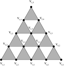
Figure 2: The graph $G_{5}$.

The graph $G_{r}$ has $\binom{r+1}{2}$ vertices, denoted as $v_{i,l}$ for $l\in[r]$ and $i\in[r-l+1]$ (with $v_{1,l},\ldots,v_{r-l+1,l}$ at level $l$, see Figure 2). Note that $G_{2}=K_{3}=F_{2}$, $G_{3}=F_{3}$, but $G_{r}\neq F_{r}$ for $r\geq 4$. Using the following lemma we can construct some points of $\mathcal{E}(G_{r})$ with a unique completion.

Lemma 4.4.

Consider a labeling of the nodes of $G_{r}$ by vectors $w_{i,l}$ satisfying the following property $(P_{r})$: For each triangle $C_{i,l}=\{v_{i,l},v_{i+1,l},v_{i,l+1}\}$ of $G_{r}$, the set $\{w_{i,l},w_{i+1,l},w_{i,l+1}\}$ is minimally linearly dependent. (These triangles are shaded in Figure 2). Let $X$ be the Gram matrix of the vectors $w_{i,l}$ and let $x=\pi_{E(G_{r})}(X)$ be its projection. Then $X$ is the unique completion of $x$.

Proof.

For $r=2$, $G_{2}=K_{3}$ and there is nothing to prove. Let $r\geq 3$ and assume that the claim holds for $r-1$. Consider a labeling $w_{i,l}$ of $G_{r}$ satisfying $(P_{r})$ and the corresponding vector $x\in\mathcal{E}(G_{r})$. We show, using Lemma 4.1, that the entries $Y_{uv}$ of a psd completion $Y$ of $x$ are uniquely determined for all $\{u,v\}\not\in E(G_{r})$. For this, denote by $H,R,L$ the sets of nodes lying on the ‘horizontal’ side, the ‘right’ side and the ‘left’ side of $G_{r}$, respectively (refer to the drawing of $G_{r}$ of Figure 2). Observe that each of $G_{r}\backslash H$, $G_{r}\backslash R$, $G_{r}\backslash L$ is a copy of $G_{r-1}$. As the induced vector labelings on each of these graphs satisfies the property $(P_{r-1})$, we can conclude using the induction assumption that the entry $Y_{uv}$ is uniquely determined whenever the pair $\{u,v\}$ is contained in the vertex set of one of $G_{r}\backslash H$, $G_{r}\backslash R$, or $G_{r}\backslash L$. The only non-edges $\{u,v\}$ that are not yet covered arise when $u$ is a corner of $G_{r}$ and $v$ lies on the opposite side, say $u=v_{1,1}$ and $v=v_{r-l+1,l}\in R$. If $l\neq 1,r$ then the clique $C_{1,1}=\{v_{1,1},v_{2,1},v_{1,2}\}$ forces the pair $\{u,v\}$ (since $\{v,v_{1,2}\}\subseteq E(G_{r}\backslash H)$ and $\{v,v_{2,1}\}\subseteq E(G_{r}\backslash L)$). If $l=r$ then the clique $C_{1,r-1}=\{v_{1,r-1},v_{2,r-1},v_{1,r}\}$ forces the pair $\{u,v\}$ (since $\{u,v_{1,r-1}\}\subseteq E(G_{r}\backslash R)$ and the value at the pair $\{u,v_{2,r-1}\}$ has just been specified). Analogously for the case $l=1$. This concludes the proof. ∎

Theorem 4.5.

We have that $\text{\rm egd}(G_{r})=r$ for all $r\geq 2$. Moreover, $G_{r}$ is a minimal forbidden minor for the class ${\mathcal{G}}_{r-1}$.

Proof.

Since $G_{r}$ has $\binom{r+1}{2}$ nodes it follows from Lemma 3.5 that $\text{\rm egd}(G_{r})\leq r$. We now show that $\text{\rm egd}(G_{r})\geq r$. For this, choose a vector labeling of the nodes of $G_{r}$ satisfying the conditions of Lemma 4.4: Label the nodes $v_{1,1},\ldots,v_{r,1}$ at level $l=1$ by the standard unit vectors $w_{1,1}=e_{1},\ldots,w_{r,1}=e_{r}$ in ${\mathbb{R}}^{r}$ and define inductively $w_{i,l+1}={w_{i,l}+w_{i+1,l}\over\|w_{i,l}+w_{i+1,l}\|}$ for $l=1,\ldots,r-1$. By Lemma 4.4 their Gram matrix $X$ is the unique completion of its projection $x=\pi_{E(G_{r})}(X)\in\mathcal{E}(G_{r})$. Moreover, $X$ is extreme in $\mathcal{E}_{n}$ since ${\mathcal{U}}_{V}$ is full-dimensional in ${\mathcal{S}}^{r}$. This shows $\text{\rm egd}(G_{r})\geq r$, by Lemma 3.6.

We now show that $\text{\rm egd}(G_{r}\backslash e)\leq r-1$. For this use the following inequalities: $\text{\rm egd}(G_{r}\backslash e)\leq{\rm la_{\boxtimes}}(G_{r}\backslash e)\leq{\rm la_{\square}}(G_{r}\backslash e)\leq r-1$, where the leftmost inequality follows from Corollary 3.12 and the rightmost one is shown in [17]. ∎

We conclude with two immediate corollaries.

Corollary 4.6.

The graph parameter $\text{\rm egd}(G)$ is unbounded for the class of planar graphs.

Corollary 4.7.

Let $T$ be a tree which contains a path with $2r-2$ nodes. Then, $\text{\rm egd}(T\boxtimes K_{r})=r$.

Proof.

It is shown in [7] that $G_{r}$ is a minor of the Cartesian product of two paths $P_{r}$ and $P_{2r-2}$ (with, respectively, $r$ and $2r-2$ nodes). Hence, $G_{r}\preceq P_{2r-2}\Box P_{r}\preceq T\boxtimes K_{r}$ and thus $r=\text{\rm egd}(G_{r})\leq\text{\rm egd}(T\boxtimes K_{r})$. ∎

4.3 The class $H_{r}$

In this section we consider a third class of graphs $H_{r}$ for every $r\geq 3$. In order to explain the general definition we first describe the base case $r=3$.

Figure 3: The graphs $H_{3}$ and $H_{4}$.

The graph $H_{3}$ is shown in Figure 3. It is obtained by taking a complete graph $K_{4}$, with vertices $v_{1},v_{2},v_{3}$ and $v_{13}$, and subdividing two adjacent edges: here we insert node $v_{12}$ between $v_{1}$ and $v_{2}$ and node $v_{23}$ between nodes $v_{2}$ and $v_{3}$.

Lemma 4.8.

$\text{\rm egd}(H_{3})=3$ and $H_{3}$ is a minimal forbidden minor for ${\mathcal{G}}_{2}$.

Proof.

As $H_{3}$ has 6 nodes, $\text{\rm egd}(H_{3})\leq 3$. To show equality, we use the following vector labeling for the nodes of $H_{3}$: Label the nodes $v_{1},v_{2},v_{3}$ by the standard unit vectors $e_{1},e_{2},e_{3}\in{\mathbb{R}}^{3}$ and $v_{ij}$ by $(e_{i}+e_{j})/\sqrt{2}$ for $1\leq i<j\leq 3$. Let $X\in\mathcal{E}_{6}$ be their Gram matrix and set $x=\pi_{E(H_{3})}(X)\in\mathcal{E}(H_{3})$. Then $X$ has rank 3 and $X$ is an extreme point of $\mathcal{E}_{6}$. We now show that $X$ is the unique completion of $x$ in $\mathcal{E}_{6}$. For this let $Y\in{\rm fib}(x)$. Consider its principal submatrices $Z,Z^{\prime}$ indexed by $\{v_{1},v_{2},v_{3},v_{13}\}$ and $\{v_{1},v_{2},v_{12}\}$, of the form:

$$Z=\left(\begin{matrix}1&a&0&\sqrt{2}/2\cr a&1&b&0\cr 0&b&1&\sqrt{2}/2\cr\sqrt{2}/2&0&\sqrt{2}/2&1\end{matrix}\right)\qquad Z^{\prime}=\left(\begin{matrix}1&a&\sqrt{2}/2\cr a&1&\sqrt{2}/2\cr\sqrt{2}/2&\sqrt{2}/2&1\end{matrix}\right),$$

where $a,b\in{\mathbb{R}}$. Then, $\det(Z)=-(a+b)^{2}/2$ implies $a+b=0$, and $\det(Z^{\prime})=a(1-a)$ implies $a\geq 0$. Similarly, $b\geq 0$ using the principal submatrix of $Y$ indexed by $\{v_{2},v_{3},v_{23}\}$. This shows $a=b=0$ and thus the entries of $Y$ at the positions $\{v_{1},v_{2}\}$ and $\{v_{2},v_{3}\}$ are uniquely specified. Remains to show that the entries are uniquely specified at the non-edges containing $v_{12}$ or $v_{23}$. For this we use Lemma 4.1: First the clique $\{v_{2},v_{3},v_{23}\}$ forces the pairs $\{v_{1},v_{23}\}$ and $\{v_{13},v_{23}\}$ and then the clique $\{v_{1},v_{2},v_{12}\}$ forces the pairs $\{v_{23},v_{12}\}$, $\{v_{13},v_{12}\}$, and $\{v_{3},v_{12}\}$. Thus we have shown $Y=X$, which concludes the proof that $\text{\rm egd}(H_{3})=3$.

We now verify that it is a minimal forbidden minor. Contracting any edge results in a graph on 5 nodes and we are done by (23). Lastly, we verify that $\text{\rm egd}(H_{3}\backslash e)\leq 2$ for each edge $e\in E(H_{3})$. If deleting the edge $e$ creates a cut node, then the result follows using Lemma 3.3. Otherwise, $H_{3}\backslash e$ is contained in $T\boxtimes K_{2}$, where $T$ is a path (for $e=\{v_{2},v_{13}\}$) or a claw $K_{1,3}$ (for $e=\{v_{1},v_{13}\}$ or $\{v_{3},v_{13}\}$), and the result follows from Theorem 3.11. ∎

We now describe the graph $H_{r}$, or rather a class ${\mathcal{H}}_{r}$ of such graphs. Any graph $H_{r}\in{\mathcal{H}}_{r}$ is constructed in the following way. Its node set is $V=V_{0}\cup V_{3}\cup\ldots\cup V_{r}$, where $V_{0}=\{v_{ij}:3\leq i<j\leq r\}$ and, for $i\in\{3,\ldots,r\}$, $V_{i}=\{v_{1},v_{2},v_{12},v_{i},v_{1i},v_{2i}\}$. So $H_{r}$ has $n={r+1\choose 2}$ nodes. Its edge set is defined as follows: On each set $V_{i}$ we put a copy of $H_{3}$ (with index $i$ playing the role of index 3 in the description of $H_{3}$ above) and, for each $3\leq i<j\leq r$, we have the edges $\{v_{i},v_{ij}\}$ and $\{v_{j},v_{ij}\}$ as well as exactly one edge, call it $e_{ij}$, from the set

$$F_{ij}=\{\{v_{i},v_{j}\},\{v_{i},v_{1j}\},\{v_{j},v_{1i}\},\{v_{1i},v_{1j}\}\}.$$ (27)

Figure 3 shows the graph $H_{4}$ for the choice $e_{34}=\{v_{4},v_{13}\}$.

Theorem 4.9.

For any graph $H_{r}\in{\mathcal{H}}_{r}$ ($r\geq 3$), $\text{\rm egd}(H_{r})=r$.

Proof.

We label the nodes $v_{1},\ldots,v_{r}$ by $e_{1},\ldots,e_{r}\in{\mathbb{R}}^{r}$ and $v_{ij}$ by $(e_{i}+e_{j})/\sqrt{2}$. Let $X\in\mathcal{E}_{n}$ be their Gram matrix and $x=\pi_{E(H_{r})}(X)\in\mathcal{E}(H_{r})$. Then $X$ is an extreme point of $\mathcal{E}_{n}$, we show that ${\rm fib}(x)=\{X\}$. For this let $Y\in{\rm fib}(x)$. We already know that $Y[V_{i}]=X[V_{i}]$ for each $i\in\{3,\ldots,r\}$. Indeed, as the subgraph of $H_{r}$ induced by $V_{i}$ is $H_{3}$, this follows from the way we have chosen the labeling and from the proof of Lemma 4.8. Hence we may now assume that we have a complete graph on each $V_{i}$ and it remains to show that the entries of $Y$ are uniquely specified at the non-edges that are not contained in some set $V_{i}$ ($3\leq i\leq r$). For this note that the vectors labeling the set $C_{ij}=\{v_{i},v_{j},v_{ij}\}$ are minimally linearly dependent. Using Lemma 4.1, one can verify that all remaining non-edges are forced using these sets $C_{ij}$ and thus $Y=X$. This shows that $\text{\rm egd}(H_{r})\geq r$. ∎

In contrast to the graphs $F_{r}$ and $G_{r}$, we do not know whether $H_{r}\in{\mathcal{H}}_{r}$ is a minimal forbidden minor for ${\mathcal{G}}_{r-1}$ for $r\geq 4$.

4.4 Two special graphs: $K_{3,3}$ and $K_{5}$

In this section we consider the graphs $K_{3,3}$ and $K_{5}$ which will play a special role in the characterization of the class ${\mathcal{G}}_{2}$. First we compute the extreme Gram dimension of $K_{3,3}$. Note that its Gram dimension is $\text{\rm gd}(K_{3,3})=4$ as $K_{3,3}$ contains a $K_{4}$-minor but it contains no $K_{5}$ and $K_{2,2,2}$-minor; cf. Theorem 1.2.

Our main goal in this section is to show that the extreme Gram dimension of the graph $K_{3,3}$ is equal to 2, i.e., for any $x\in{\rm ext\hskip 1.42262pt}\mathcal{E}(K_{3,3})$ there exists a psd completion of rank at most 2. We start by showing that any completion of an element of ${\rm ext\hskip 1.42262pt}\mathcal{E}(K_{3,3})$ has rank at most 3.

Lemma 4.10.

For $x\in{\rm ext\hskip 1.42262pt}\mathcal{E}(K_{3,3})$, any $X\in{\rm fib}(x)$ has rank at most 3.

Proof.

Let $x\in{\rm ext\hskip 1.42262pt}\mathcal{E}(K_{3,3})$ and let $X\in{\rm fib}(x)$ with ${\rm rank\hskip 1.42262pt}X\geq 4$. Let $u_{1},\ldots,u_{6}$ be a Gram representation of $X$ and choose a subset $\{u_{i}:i\in I\}$ of linearly independent vectors with $|I|=4$. Let $E_{I}$ denote the set of edges of $K_{3,3}$ induced by $I$ and set

$${\mathcal{U}}_{I}=\{U_{ii}:i\in I\}\cup\{U_{ij}:\{i,j\}\in E_{I}\}.$$

Then ${\mathcal{U}}_{I}$ consists of linearly independent elements; cf. Lemma 3.10. By Lemma 2.3, ${\mathcal{U}}_{I}$ is contained in $\{{\mathcal{U}}_{ii}:i\in[6]\}$ and thus it has dimension at most 6. On the other hand, as any four nodes induce at least three edges in $K_{3,3}$, we have that $|{\mathcal{U}}_{I}|\geq 4+3=7$ and thus the dimension of ${\mathcal{U}}_{I}$ is at least 7, a contradiction. ∎

The proof of the main theorem relies on the following two lemmas.

Lemma 4.11.

Let $X,Z\in{\mathcal{S}}^{n}$ with $X\succeq 0$ and satisfying:

$$Xz=0\Longrightarrow z^{\sf T}Zz\geq 0,\ \ Xz=0,z^{\sf T}Zz=0\Longrightarrow Zz=0.$$ (28)

Then $X+tZ\succeq 0$ for some $t>0$.

Proof.

Up to an orthogonal transformation we may assume $X=\left(\begin{matrix}D&0\cr 0&0\end{matrix}\right)$, where $D$ is a diagonal matrix with positive diagonal entries. Correspondingly, write $Z$ in block form: $Z=\left(\begin{matrix}A&B\cr B^{\sf T}&C\end{matrix}\right)$. The conditions (28) show that $C\succeq 0$ and that the kernel of $C$ is contained in the kernel of $B$. This implies that $X+tZ\succeq 0$ for some $t>0$. ∎

Lemma 4.12.

Let $x\in{\rm ext\hskip 1.42262pt}\mathcal{E}(K_{3,3})$, let $X\in{\rm ext\hskip 1.42262pt}{\rm fib}(x)$ with ${\rm rank\hskip 1.42262pt}X=3$ and with Gram representation $\{u_{1},\ldots,u_{6}\}\subseteq{\mathbb{R}}^{3}$. Let $V_{1}=\{1,2,3\}$ and $V_{2}=\{4,5,6\}$ be the bipartition of the node set of $K_{3,3}$. Then, there exist matrices $Y_{1},Y_{2}\in{\mathcal{S}}^{3}$ such that $Y_{1}+Y_{2}\succ 0$ and

$$\langle Y_{k},U_{ii}\rangle=0\ \forall i\in V_{k}\ \forall k\in\{1,2\}\ \text{ and }\ \exists k\in\{1,2\}\ \exists i,j\in V_{k}\ \langle Y_{k},U_{ij}\rangle\neq 0.$$

Proof.

Define ${\mathcal{U}}_{k}=\langle U_{ii}:i\in V_{k}\rangle\subseteq{\mathcal{W}}_{k}=\langle U_{ij}:i,j\in V_{k}\rangle\subseteq{\mathcal{S}}^{3}$ for $k=1,2$. With this notation we are looking for two matrices $Y_{1},Y_{2}$ such that $Y_{1}+Y_{2}\succ 0,Y_{1}\in{\mathcal{U}}_{1}^{\perp},Y_{2}\in{\mathcal{U}}_{2}^{\perp}$ and either $Y_{1}\not\in{\mathcal{W}}_{1}^{\perp}$ or $Y_{2}\not\in{\mathcal{W}}_{2}^{\perp}$.

Since $x\in{\rm ext\hskip 1.42262pt}\mathcal{E}(K_{3,3})$ by Lemma 2.4 it follows that ${\rm fib}(x)$ is a face of $\mathcal{E}_{6}$ and by (13) we have that $X\in{\rm ext\hskip 1.42262pt}\mathcal{E}_{6}$. Then (17) implies that $\dim\langle U_{ii}:i\in[6]\rangle=6$ and thus $\dim{\mathcal{U}}_{1}=\dim{\mathcal{U}}_{2}=3$. This implies that ${\mathcal{U}}_{1}\cap{\mathcal{U}}_{2}=\{0\}$ and thus ${\mathcal{U}}_{1}^{\perp}\cup{\mathcal{U}}_{2}^{\perp}={\mathcal{S}}^{3}$. Moreover, as $\dim{\mathcal{U}}_{1}^{\perp}=\dim{\mathcal{U}}_{2}^{\perp}=3$ it follows that ${\mathcal{U}}_{1}^{\perp}\cap{\mathcal{U}}_{2}^{\perp}=\{0\}$ and thus ${\mathcal{S}}^{3}={\mathcal{U}}_{1}^{\perp}\oplus{\mathcal{U}}_{2}^{\perp}$. Lastly, we have that ${\mathcal{W}}_{k}^{\perp}\subseteq{\mathcal{U}}_{k}^{\perp}\ (k=1,2)$ and thus ${\mathcal{W}}_{1}^{\perp}\cap{\mathcal{W}}_{2}^{\perp}\subseteq{\mathcal{U}}_{1}^{\perp}\cap{\mathcal{U}}_{2}^{\perp}=\{0\}.$

Assume for contradiction that ${\mathcal{S}}^{3}_{++}$ is contained in ${\mathcal{W}}_{1}^{\perp}\oplus{\mathcal{W}}_{2}^{\perp}$. This implies that

$${\mathcal{W}}_{1}^{\perp}\oplus{\mathcal{W}}_{2}^{\perp}={\mathcal{S}}^{3}={\mathcal{U}}_{1}^{\perp}\oplus{\mathcal{U}}_{2}^{\perp}$$ (29)

and thus ${\mathcal{W}}_{k}={\mathcal{U}}_{k}\ (k=1,2)$. Indeed, (29) implies that $\dim{\mathcal{W}}_{1}^{\perp}+\dim{\mathcal{W}}_{2}^{\perp}=\dim{\mathcal{U}}_{1}^{\perp}+\dim{\mathcal{U}}_{2}^{\perp}$ which combined with the fact that ${\mathcal{W}}_{k}^{\perp}\subseteq{\mathcal{U}}_{k}^{\perp}\ (k=1,2)$ gives that $\dim{\mathcal{W}}_{k}^{\perp}=\dim{\mathcal{U}}_{k}^{\perp}\ (k=1,2)$. Lastly, using the fact that ${\mathcal{U}}_{k}\subseteq W_{k}\ (k=1,2)$ the claim follows. In turn this implies that ${\mathcal{W}}_{1}\cap{\mathcal{W}}_{2}={\mathcal{U}}_{1}\cap{\mathcal{U}}_{2}=\{0\}$.

As $\dim{\mathcal{U}}_{k}=3$, we have $\dim\langle u_{i}:i\in V_{k}\rangle\geq 2$ for $k=1,2$. Say, $\{u_{1},u_{2}\}$ and $\{u_{4},u_{5}\}$ are linearly independent. As $\dim\langle u_{i}:i\in[6]\rangle=3$, there exists a nonzero vector $\lambda\in{\mathbb{R}}^{4}$ such that $0\neq w=\lambda_{1}u_{1}+\lambda_{2}u_{2}=\lambda_{3}u_{4}+\lambda_{4}u_{5}$. Notice that the scalar $w$ is nonzero for otherwise the vectors $u_{1},u_{2}$ would be dependent. Hence we obtain that $ww^{\sf T}\in{\mathcal{W}}_{1}\cap{\mathcal{W}}_{2}$, contradicting the fact that ${\mathcal{W}}_{1}\cap{\mathcal{W}}_{2}=\{0\}$.

Hence we have shown that ${\mathcal{S}}^{3}_{++}\not\subseteq{\mathcal{W}}_{1}^{\perp}\oplus{\mathcal{W}}_{2}^{\perp}$. So there exists a positive definite matrix $Y$ which does not belong to ${\mathcal{W}}_{1}^{\perp}\oplus{\mathcal{W}}_{2}^{\perp}$. Write $Y=Y_{1}+Y_{2}$, where $Y_{k}\in{\mathcal{U}}_{k}^{\perp}$ for $k=1,2$. We may assume, say, that $Y_{1}\not\in{\mathcal{W}}_{1}^{\perp}$. Thus $Y_{1},Y_{2}$ satisfy the lemma. ∎

We can now show the main result of this section.

Theorem 4.13.

For the graph $K_{3,3}$ we have that $\text{\rm egd}(K_{3,3})=2$, i.e., for any partial matrix $x\in{\rm ext\hskip 1.42262pt}\mathcal{E}(K_{3,3})$ there exists a completion $X\in{\rm fib}(x)$ with ${\rm rank\hskip 1.42262pt}X\leq 2$.

Proof.

Let $x\in{\rm ext\hskip 1.42262pt}\mathcal{E}(K_{3,3})$ and let $X\in{\rm fib}(x)$ be an extreme point of $\mathcal{E}_{6}$ (which exists by Lemma 2.4 (ii)). We assume that ${\rm rank\hskip 1.42262pt}X=3$ (else we are done). Let $\{u_{1},\ldots,u_{6}\}\subseteq{\mathbb{R}}^{3}$ be a Gram representation of $X$ and let $Y_{1}$ and $Y_{2}$ be the matrices provided by Lemma 4.12. Moreover, define the matrix $Z\in{\mathcal{S}}^{6}$ by $Z_{ij}=\langle Y_{k},U_{ij}\rangle$ for $i,j\in V_{k},$ $k\in\{1,2\}$, and $Z_{ij}=0$ for $i\in V_{1}$, $j\in V_{2}$. By Lemma 4.12, $Z$ is a nonzero matrix with zero diagonal entries and with zeros at the positions corresponding to the edges of $K_{3,3}$.

Next we show that $X+tZ\succeq 0$ for some $t>0$, using Lemma 4.11. For this it is enough to verify that (28) holds. Assume $Xz=0$, i.e., $a:=\sum_{i\in V_{1}}z_{i}u_{i}=-\sum_{j\in V_{2}}z_{j}u_{j}$. Then,

$$z^{\sf T}Zz=\sum_{k=1,2}\sum_{i,j\in V_{k}}z_{i}z_{j}\langle Y_{k},U_{ij}\rangle=\langle Y_{1}+Y_{2},aa^{\sf T}\rangle\geq 0,$$

since $Y_{1}+Y_{2}\succ 0$. Moreover, $z^{\sf T}Zz=0$ implies $a=0$ and thus $Zz=0$ since, for $i\in V_{k}$, $(Zz)_{i}=\sum_{j\in V_{k}}\langle Y_{k},U_{ij}\rangle z_{j}=\pm\langle Y_{k},(u_{i}a^{\sf T}+au_{i}^{\sf T})/2\rangle$. Hence, the matrix $X+tZ$ also belongs to the fiber of $x$. This shows that $|{\rm fib}(x)|\geq 2$. As, by Lemma 4.10, all matrices in ${\rm fib}(x)$ have rank at most 3, it follows that ${\rm fib}(x)$ contains a matrix of rank at most 2 (indeed, any matrix in the relative interior of ${\rm fib}(x)$ has rank 3 and any matrix on the boundary has rank at most 2). ∎

We now know that both graphs $K_{3,3}$ and $K_{5}$ belong to the class ${\mathcal{G}}_{2}$. We next show that they are in some sense maximal for this property.

Lemma 4.14.

Let $G$ be a 2-connected graph that contains $K_{5}$ or $K_{3,3}$ as a proper subgraph. Then, $G$ contains $H_{3}$ as a minor and thus $\text{\rm egd}(G)\geq 3$.

Proof.

The proof is based on the following observations. If $G$ is a 2-connected graph containing $K_{5}$ or $K_{3,3}$ as a proper subgraph, then $G$ has a minor $H$ which is one of the following graphs: (a) $H$ is $K_{5}$ with one more node adjacent to two nodes of $K_{5}$, (b) $H$ is $K_{3,3}$ with one more edge added, (c) $H$ is $K_{3,3}$ with one more node adjacent to two adjacent nodes of $K_{3,3}$. Then $H$ contains a $H_{3}$ subgraph in cases (a) and (b), and a $H_{3}$ minor in case (c) (easy verification). Hence, $\text{\rm egd}(G)\geq\text{\rm egd}(H_{3})=3$. ∎

We conclude this section with a lemma that will be used in the proof of Theorem 5.4.

Lemma 4.15.

Let $G$ be a 2-connected graph with $n\geq 6$ nodes. Then,

• If $G$ has no $F_{3}$-minor then $\omega(G)\leq 4$.

• If $G$ is chordal and has no $F_{3}$-subgraph then $\omega(G)\leq 4$.

Proof.

Assume for contradiction that $\omega(G)\geq 5$ and let $U\subseteq V$ with $G[U]=K_{5}$. Since $G$ is 2-connected and $n\geq 6$, there exists a node $u\not\in U$ which is connected by two vertex disjoint paths to two distinct nodes $v,w\in U$; let $P_{uv}$ and $P_{uw}$ be such shortest paths. In case $(i)$, contract the paths $P_{uv}$ and $P_{uw}$ to get a node adjacent to both $v$ and $w$. Then, we can easily see that $G$ has an $F_{3}$-minor, a contradiction. In case $(ii)$, let $v^{\prime}\in P_{uv}$ and $w^{\prime}\in P_{uw}$ with $(v,v^{\prime}),(w,w^{\prime})\in E(G)$. Since $G$ is chordal and the paths are the shortest possible, at least one of the edges $(v,w^{\prime})$ or $(w,v^{\prime})$ will be present in $G$. This implies that $G$ contains an $F_{3}$-subgraph, a contradiction. ∎

5 Graphs with extreme Gram dimension at most 2

In this section we characterize the class ${\mathcal{G}}_{2}$ of graphs with extreme Gram dimension at most 2. Our main result is the following:

Theorem 5.1.

For any graph $G$,

$$\text{\rm egd}(G)\leq 2\text{ if and only if }G\text{ has no minors }F_{3}\text{ or }H_{3}.$$

The graphs $F_{3}$ and $H_{3}$ are illustrated in Figure 4 below.

Figure 4: The graphs $F_{3}$ and $H_{3}$

In the previous sections we established that the graphs $F_{3}$ and $H_{3}$ are minimal forbidden minors for the class of graphs satisfying $\text{\rm egd}(G)\leq 2$. In order to prove Theorem 5.1 it remains to show that a graph $G$ having no $F_{3}$ and $H_{3}$ minors satisfies $\text{\rm egd}(G)\leq 2$.

By Lemma 3.3 we may assume that $G$ is 2-connected. Moreover, we may assume that $|V(G)|\geq 6$, since for graphs on at most five nodes we know that $\text{\rm egd}(G)\leq\text{\rm egd}(K_{5})=2$ (recall (23)). Additionally, since $\text{\rm egd}(K_{3,3})=2$ (recall Theorem 4.13) we may also assume that $G\neq K_{3,3}$.

Consequently, it suffices to consider 2-connected graphs with at least 6 nodes that are different from $K_{3,3}$. Then, Theorem 5.1 follows from the equivalence of the first two items in the next theorem.

Theorem 5.2.

Let $G$ be a 2-connected graph with $n\geq 6$ nodes and $G\neq K_{3,3}$. Then, the following assertions are equivalent.

• $\text{\rm egd}(G)\leq 2$.

• $G$ has no minors $F_{3}$ or $H_{3}$.

• ${\rm la_{\boxtimes}}(G)\leq 2$, i.e., $G$ is a minor of $T\boxtimes K_{2}$ for some tree $T$.

The implication $(i)\Longrightarrow(ii)$ follows from Theorem 4.2 and Theorem 4.8. Moreover, the implication $(iii)\Longrightarrow(i)$ follows from Theorem 3.11. The rest of this chapter is dedicated to proving the implication $(ii)\Longrightarrow(iii).$ The proof consists of two steps. First we consider the chordal case and show:

• The chordal case: Let $G$ be a 2-connected chordal graph with $n\geq 6$ nodes. Then, $G$ has no $F_{3}$ or $H_{3}$-minors if and only if $G$ is a contraction minor of $T\boxtimes K_{2}$, for some tree $T$ (Section 5.1, Theorem 5.4).

Then, we reduce the general case to the chordal case and show:

• Reduction to the chordal case: Let $G$ be a 2-connected graph with $n\geq 6$ nodes and $G\neq K_{3,3}$. If $G$ has no $F_{3}$ or $H_{3}$-minors then $G$ is a subgraph of a chordal graph with no $F_{3}$ or $H_{3}$-minors.

Notice that, in case (1), $G$ is by assumption chordal and thus the case $G=K_{3,3}$ is automatically excluded. For case (2), we first need to exclude $K_{4}$ instead of $H_{3}$ (Section 5.2, Theorem 5.7) and then we derive from this special case the general result (Section 5.3, Theorem 5.12).

5.1 The chordal case

Our goal in this section is to characterize the $2$-connected chordal graphs $G$ with $\text{\rm egd}(G)\leq 2$. By Lemma 4.14, if $G\neq K_{5}$ has $\text{\rm egd}(G)\leq 2$, then $\omega(G)\leq 4$. Throughout this section we denote by ${\mathcal{C}}$ the family of all 2-connected chordal graphs with $\omega(G)\leq 4$. Any graph $G\in{\mathcal{C}}$ is a clique 2- or 3-sum of $K_{3}$’s and $K_{4}$’s. Note that $F_{3}$ belongs to ${\mathcal{C}}$ and has $\text{\rm egd}(F_{3})=3$. On the other hand, any graph $G=T\boxtimes K_{2}$ where $T$ is a tree, belongs to ${\mathcal{C}}$ and has $\text{\rm egd}(G)=2$. These graphs are “special clique 2-sums” of $K_{4}$’s, as they satisfy the following property: every 4-clique has at most two edges which are cutsets and these two edges are not adjacent. This motivates the following definitions, useful in the proof of Theorem 5.4 below.

Definition 5.3.

Let $G$ be a 2-connected chordal graph with $\omega(G)\leq 4$.

• An edge of $G$ is called free if it belongs to exactly one maximal clique and non-free otherwise.

• A 3-clique in $G$ is called free if it contains at least one free edge.

• A 4-clique in $G$ is called free if it does not have two adjacent non-free edges. A free 4-clique can be partitioned as $\{a,b\}\cup\{c,d\}$, called its two sides, where only $\{a,b\}$ and $\{c,d\}$ can be non-free.

• $G$ is called free if all its maximal cliques are free.

For instance, $F_{3}$, $K_{5}\setminus e$ (the clique 3-sum of two $K_{4}$’s) are not free. Hence any free graph in ${\mathcal{C}}$ is a clique 2-sum of free $K_{3}$’s and free $K_{4}$’s. Note also that ${\rm la_{\boxtimes}}(K_{5}\setminus e)=3$. We now show that for a graph $G\in{\mathcal{C}}$ the property of being free is equivalent to having ${\rm la_{\boxtimes}}(G)\leq 2$ and also to having $\text{\rm egd}(G)\leq 2$.

Theorem 5.4.

Let $G$ be a 2-connected chordal graph with $n\geq 6$ nodes. The following assertions are equivalent:

• $G$ has no minors $F_{3}$ or $H_{3}$.

• $G$ does not contain $F_{3}$ as a subgraph.

• $\omega(G)\leq 4$ and $G$ is free.

• $G$ is a contraction minor of $T\boxtimes K_{2}$ for some tree $T$.

• ${\rm la_{\boxtimes}}(G)\leq 2.$

• $\text{\rm egd}(G)\leq 2$.

Proof.

The implication $(i)\Rightarrow(ii)$ is clear and the implications $(iv)\Rightarrow(v)\Rightarrow(vi)\Rightarrow(i)$ follow from earlier results.

$(ii)\Rightarrow(iii)$: Assume that $(ii)$ holds. By Lemma 4.15 $(ii)$ it follows that $\omega(G)~{}\leq 4$. Our first goal is to show that $G$ does not contain clique 3-sums of $K_{4}$’s, i.e., it does not contain a $K_{5}\setminus e$ subgraph. For this, assume that $G[U]=K_{5}\backslash e$ for some $U\subseteq V(G)$. As $|V(G)|\geq 6$ and $G$ is 2-connected chordal, there exists a node $u\not\in U$ which is adjacent to two adjacent nodes of $U$. Then, one can find a $F_{3}$ subgraph in $G$, a contradiction. Therefore, $G$ is a clique 2-sum of $K_{3}$’s and $K_{4}$’s. We now show that each of them is free.

Suppose first that $C=\{a,b,c\}$ is a maximal 3-clique which is not free. Then, there exist nodes $u,v,w\not\in C$ such that $\{a,b,u\}$, $\{a,c,v\}$, $\{b,c,w\}$ are cliques in $G$. Moreover, $u,v,w$ are pairwise distinct (if $u=v$ then $C\cup\{u\}$ is a clique, contradicting maximality of $C$) and we find a $F_{3}$ subgraph in $G$.

Suppose now that $C=\{a,b,c,d\}$ is a 4-clique which is not free and, say, both edges $\{a,b\}$ and $\{a,c\}$ are non-free. Then, there exist nodes $u,v\not\in C$ such that $\{a,b,u\}$ and $\{a,c,v\}$ are cliques. Moreover, $u\neq v$ (else we find a $K_{5}\backslash e$ subgraph) and thus we find a $F_{3}$ subgraph in $G$. Thus (iii) holds.

$(iii)\Rightarrow(iv):$ Assume that $G$ is free, $G\neq K_{4},K_{3}$ (else we are done). When all maximal cliques are 4-cliques, it is easy to show using induction on $|V(G)|$ that $G=T\boxtimes K_{2}$, where $T$ is a tree and each side of a 4-clique of $G$ corresponds to a node of $T$.

Assume now that $G$ has a maximal 3-clique $C=\{a,b,c\}$. Say, $\{b,c\}$ is free and $\{a,b\}$ is a cutset. Write $V(G)=V^{\prime}\cup V^{\prime\prime}\cup\{a,b\}$, where $V^{\prime\prime}$ is the (vertex set of the) component of $G\backslash\{a,b\}$ containing $c$, and $V^{\prime}$ is the union of the other components. Now replace node $a$ by two new nodes $a^{\prime},a^{\prime\prime}$ and replace $C$ by the 4-clique $C^{\prime}=\{a^{\prime},a^{\prime\prime},b,c\}$. Moreover, replace each edge $\{u,a\}$ by $\{u,a^{\prime}\}$ if $u\in V^{\prime}$ and by $\{u,a^{\prime\prime}\}$ if $u\in V^{\prime\prime}$. Let $G^{\prime}$ be the graph obtained in this way. Then $G^{\prime}\in{\mathcal{C}}$ is free, $G^{\prime}$ has one less maximal 3-clique than $G$, and $G=G^{\prime}/\{a^{\prime},a^{\prime\prime}\}$. Iterating, we obtain a graph $\widehat{G}$ which is a clique 2-sum of free $K_{4}$’s and contains $G$ as a contraction minor. By the above, $\widehat{G}=T\boxtimes K_{2}$ and thus $G$ is a contraction minor of $T\boxtimes K_{2}$. ∎

5.2 Structure of the graphs with no $F_{3}$ and $K_{4}$-minor

In this section we investigate the structure of the graphs with no $F_{3}$ or $K_{4}$-minors. We start with two technical lemmas.

Lemma 5.5.

Let $G$ and $M$ be two $2$-connected graphs, let $\{x,y\}\not\in E(G)$ be a cutset in $G$, and let $r\geq 2$ be the number of components of $G\setminus\{x,y\}$.

• Assume that $G\in\mathcal{F}(M)$, but the graph $G+\{x,y\}$ has a $M$-minor with $M$-partition $\{V_{i}:i\in V(M)\}$. If $x\in V_{i}$ and $y\in V_{j}$, then $M\setminus\{i,j\}$ has at least $r\geq 2$ components (and thus $i\neq j$).

• Assume that $M$ does not have two adjacent nodes forming a cutset in $M$. If $G\in{\mathcal{F}}(M)$, then $G+\{x,y\}\in{\mathcal{F}}(M)$.

Proof.

(i) Let $C_{1},\ldots,C_{r}\subseteq V(G)$ be the node sets of the components of $G\setminus\{x,y\}$. As $G$ is $2$-connected, there is an $x-y$ path $P_{s}$ in $G[C_{s}\cup\{x,y\}]$ for each $s\in[r]$. Notice that $P_{s}\neq\{x,y\}$ since $P_{s}$ is a path in $G$. Our first goal is to show that every component of $M\setminus\{i,j\}$ corresponds to exactly one component of $G\setminus\{x,y\}$. For this, let $U$ be a component of $M\setminus\{i,j\}$. By the definition of the $M$-partition, the graph $G[\bigcup_{k\in U}V_{k}]$ is connected. As $x,y\not\in\bigcup_{k\in U}V_{k}$, we deduce that $\bigcup_{k\in U}V_{k}\subseteq C_{s}$ for some $s\in[r]$. We can now conclude the proof. Assume for contradiction that $M\setminus\{i,j\}$ has less than $r$ components. Then there is at least one component $C_{s}$ which does not correspond to any component of $M\setminus\{i,j\}$ which means that $(\bigcup_{k\neq i,j}V_{k})\cap C_{s}=\emptyset$. Indeed, if $V_{k}\cap C_{s}$ for some $k\neq i,j$ then since $C_{s}$ is a connected component of $G\setminus\{x,y\}$ it follows that $\cup_{\lambda\in U}V_{\lambda}\subseteq C_{s}$, where $U$ is the component of $M\setminus\{i,j\}$ that contains $k$. Summarizing we know that $C_{s}\subseteq V_{i}\cup V_{j}$. Hence the path $P_{s}$ is contained in $G[V_{i}\cup V_{j}]$, thus $\{V_{i}:i\in V(M)\}$ remains an $M$-partition of $G$ (recall that $P_{s}\neq\{x,y\}$) and we find a $M$-minor in $G$, a contradiction. Therefore, $M\setminus\{i,j\}$ has at least $r\geq 2$ components. This implies that $\{i,j\}$ is a cutset of $M$ since $M$ is 2-connected it follows that $i\neq j$.

(ii) Assume $G+\{x,y\}$ has a $M$-minor, with corresponding $M$-partition $\{V_{i}:i\in V(M)\}$. By (i), the nodes $x$ and $y$ belong to two distinct classes $V_{i}$ and $V_{j}$ and $\{i,j\}$ is a cutset in $M$. By the hypothesis, this implies that $\{i,j\}\not\in E(M)$ and thus $M$ is a minor of $G$, a contradiction. ∎

We continue with a lemma that will be essential for the next theorem.

Lemma 5.6.

Let $G\in{\mathcal{F}}(K_{4})$ be a 2-connected graph and let $\{x,y\}\not\in E(G)$. If there are at least three (internally vertex) disjoint paths from $x$ to $y$, then $\{x,y\}$ is a cutset and $G\backslash\{x,y\}$ has at least 3 components.

Proof.

Let $P_{1},P_{2},P_{3}$ be distinct vertex disjoint paths from $x$ to $y$. Then $P_{1}\setminus\{x,y\}$, $P_{2}\setminus\{x,y\}$ and $P_{3}\setminus\{x,y\}$ lie in distinct components of $G\setminus\{x,y\}$, for otherwise $G$ would contain a homeomorph of $K_{4}$. ∎

We now arrive at the main result of this section.

Theorem 5.7.

Let $G\in{\mathcal{F}}(F_{3},K_{4})$ be a 2-connected graph on $n\geq 6$ nodes. Then, there exists a chordal graph $Q\in{\mathcal{F}}(F_{3},K_{4})$ containing $G$ as a subgraph.

Proof.

Let $G$ be a 2-connected graph in ${\mathcal{F}}(F_{3},K_{4})$. As a first step, consider $\{x,y\}\not\in E(G)$ such that there exist at least three disjoint paths in $G$ from $x$ to $y$. Then, Lemma 5.6 implies that $\{x,y\}$ is a cutset of $G$ and $G\setminus\{x,y\}$ has at least three components. As a first step we show that we can add the edge $\{x,y\}$ without creating a $K_{4}$ or $F_{3}$-minor, i.e., $G+\{x,y\}\in{\mathcal{F}}(F_{3},K_{4})$.

As $\{x,y\}$ is a cutset, Lemma 5.5 (ii) applied for $M=K_{4}$ gives that $G+\{x,y\}$ does not have a $K_{4}$ minor. Assume for contradiction that $G+\{x,y\}$ has an $F_{3}$ minor. Again, Lemma 5.5 (i) applied for $M=F_{3}$ implies that $x\in V_{i},y\in V_{j},$ where $F_{3}\setminus\{i,j\}$ has at least 3 components. Clearly there is no such pair of vertices in $F_{3}$ so we arrived at a contradiction. Consequently, we can add edges iteratively until we obtain a graph $\widehat{G}\in{\mathcal{F}}(F_{3},K_{4})$ containing $G$ as a subgraph and satisfying:

$$\forall\{x,y\}\not\in E(\widehat{G})\ \text{ there are at most two disjoint }x-y\text{ paths in }\widehat{G}.$$ (30)

If $\widehat{G}$ is chordal we are done. So consider a chordless circuit $C$ in $\widehat{G}$. Note that any circuit $C^{\prime}$ distinct from $C$, which meets $C$ in at least two nodes, meets $C$ in exactly two nodes (if they meet in at least 3 nodes then we can find a $F_{3}$ minor) that are adjacent (if they are not adjacent then there exist three internally vertex disjoint paths between them, contradicting (30)). Call an edge of $C$ busy if it is contained in some circuit $C^{\prime}\neq C$. If $e_{1}\neq e_{2}$ are two busy edges of $C$ and $C_{i}\neq C$ is a circuit containing $e_{i}$, then $C_{1},C_{2}$ are (internally) disjoint (use (30)). Hence $C$ can have at most two busy edges, for otherwise one would find a $F_{3}$-minor in $\widehat{G}$.

We now show how to triangulate $C$ without creating a $K_{4}$ or $F_{3}$-minor: If $C$ has two busy edges denoted, say, $\{v_{1},v_{2}\}$ and $\{v_{k},v_{k+1}\}$ (possibly $k=2$), then we add the edges $\{v_{1},v_{i}\}$ for $i\in\{3,\ldots,k\}$ and the edges $\{v_{k},v_{i}\}$ for $i\in\{k+2,\ldots,|C|\}$, see Figure 5 a). If $C$ has only one busy edge $\{v_{1},v_{2}\}$, add the edges $\{v_{1},v_{i}\}$ for $i\in\{3,\ldots,|C|-1\}$, see Figure 5 b). (If $C$ has no busy edge then $G=C$, triangulate from any node and we are done).

Figure 5: Triangulating a chordless circuit with a) two or b) one busy edge.

Let $Q$ denote the graph obtained from $\widehat{G}$ by triangulating all its chordless circuits in this way. Hence $Q$ is a chordal extension of $\widehat{G}$ (and thus of $G$). We show that $Q\in{\mathcal{F}}(F_{3},K_{4})$. First we see that $Q\in{\mathcal{F}}(K_{4})$ by applying iteratively Lemma 5.5 (ii) (for $M=K_{4}$): For each $i\in\{3,\ldots,k\}$, $\{v_{1},v_{i}\}$ is a cutset of $\widehat{G}$ and of $\widehat{G}+\{\{v_{1},v_{j}\}:j\in\{3,\ldots,i-1\}\}$ (and analogously for the other added edges $\{v_{k},v_{i}\}$). Hence $Q$ is a clique 2-sum of triangles. We now verify that each triangle is free which will conclude the proof, using Theorem 5.4.

For this let $\{a,b,c\}$ be a triangle in $Q$. First note that if (say) $\{a,b\}\in E(Q)\setminus E(\widehat{G})$, then $a,b,c$ lie on a common chordless circuit $C$ of $\widehat{G}$. Indeed, let $C$ be a chordless circuit of $\widehat{G}$ containing $a,b$ and assume $c\not\in C$. By (30), $\widehat{G}\setminus\{a,b\}$ has at most two components and thus there is a path from $c$ to one of the two paths composing $C\setminus\{a,b\}$. Together with the triangle $\{a,b,c\}$ this gives a homeomorph of $K_{4}$ in $Q$, contradicting $Q\in{\mathcal{F}}(K_{4})$, just shown above. Hence the triangle $\{a,b,c\}$ lies in $C$ and thus has a free edge.

Suppose now that $\{a,b,c\}$ is a triangle contained in $\widehat{G}$. If it is not free then there is a $F_{3}$ on $\{a,b,c,x,y,z\}$ where $x$ (resp., $y$, and $z$) is adjacent to $a,b$ (resp., $a,c$, and $b,c$). Say $\{x,a\}\in E(Q)\setminus E(\widehat{G})$ (as there is no $F_{3}$ in $\widehat{G}$). Then $x,a,b$ lie on a chordless circuit $C$ of $\widehat{G}$ and $\{x,b\}\in E(\widehat{G})$ (since $\{a,b\}$ is a busy edge). Moreover, $c,y,z\not\in C$ for otherwise we get a $K_{4}$-minor in $Q$. Then delete the edge $\{x,a\}$ and replace it by the $\{x,a\}$-path along $C$. Do the same for any other edge of $E(Q)\setminus E(\widehat{G})$ connecting $y$ and $z$ to $\{a,b,c\}$. After that we get a $F_{3}$-minor in $\widehat{G}$, a contradiction. ∎

5.3 Structure of the graphs with no $F_{3}$ and $H_{3}$-minor

Here we investigate the graphs $G$ in the class ${\mathcal{F}}(F_{3},H_{3})$. By the results in Section 5.2 we may assume that $G$ contains some homeomorph of $K_{4}$. Figure 6 shows a homeomorph of $K_{4}$, where the original nodes are denoted as 1,2,3,4 and called its corners, and the wiggled lines correspond to subdivided edges (i.e., to paths $P_{ij}$ between the corners $i\neq j\in[4]$).

Figure 6: A homeomorph of $K_{4}$ and its two sides (cf. Lemma 5.8)

To help the reader visualize $F_{3}$ and $H_{3}$ we use Figure 7. Notice the special role of node $5$ in $H_{3}$ (denoted by a square) and of the (dashed) triangle $\{1,2,3\}$.

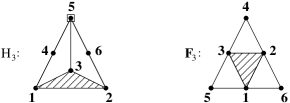
Figure 7: The graphs $H_{3}$ and $F_{3}$.

The starting point of the proof is to investigate the structure of homeomorphs of $K_{4}$ in a graph of ${\mathcal{F}}(H_{3})$.

Lemma 5.8.

Let $G$ be a 2-connected graph in $\mathcal{F}(H_{3})$ on $n\geq 6$ nodes and let $H$ be a homeomorph of $K_{4}$ contained in $G$. Then there is a partition of the corner nodes of $H$ into $\{1,3\}$ and $\{2,4\}$ for which the following holds.

• Only the paths $P_{13}$ and $P_{24}$ can have more than two nodes.

• Every component of $G\setminus H$ is connected to $P_{13}$ or to $P_{24}$.

Then $P_{13}$ and $P_{24}$ are called the two sides of $H$ (cf. Figure 6).

Proof.

We use the graphs from Figure 8 which all contain a subgraph $H_{3}$.
Case 1: $H=K_{4}$. If $G\setminus H$ has a unique component $C$ then $|C|\geq 2$ as $n\geq 6$. If $C$ is connected to two nodes of $H$, then the conclusion of the lemma holds. Otherwise, $C$ is connected to at least three nodes in $H$ and then the graph from Figure 8 a) is a minor of $G$, a contradiction.

If there are at least two components in $G\setminus H$, then they cannot be connected to two adjacent edges of $H$ for, otherwise, the graph of Figure 8 b) is a minor of $G$, a contradiction. Hence the lemma holds.

Case 2: $H\neq K_{4}$. Say, $P_{13}$ has at least 3 nodes. Then the edges $\{1,i\}$, $\{3,i\}$ ($i=2,4$) cannot be subdivided (else $H$ is a homeomorph of $H_{3}$). So (i) holds. We now show (ii). Indeed, if a component of $G\setminus H$ is connected to both $P_{13}$ and $P_{24}$, then at least one of the graphs in Figure 8 c) and d) will be a minor of $G$, a contradiction. ∎

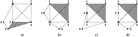
Figure 8: Bad subgraphs in the proof of Lemma 5.8.

Lemma 5.8 implies that there is no path with at least 3 nodes between the sides of a $K_{4}$-homeomorph. We now show that, moreover, there is no additional edge between the two sides. More precisely:

Lemma 5.9.

Let $G\neq K_{3,3}$ be a 2-connected graph in $\mathcal{F}(H_{3})$ on $n\geq 6$ nodes and let $H$ be a homeomorph of $K_{4}$ contained in $G$. Then there exists no edge between the two sides of $H$ except between their endpoints.

Proof.

Say, $P_{13}$ and $P_{24}$ are the two sides of $H$. Assume for a contradiction that $\{a,b\}\in E(G)$, where $a$ lies on $P_{13}$ and $b$ on $P_{24}$.

Assume first that $a$ is an internal node of $P_{13}$ and $b$ is an internal node of $P_{24}$. If $|V(H)|=6$, then $H=K_{3,3}$ and Lemma 4.14 implies that $G$ has a $H_{3}$ minor, a contradiction. Hence, $|V(H)|>6$ and we can assume w.l.o.g. that the path from $1$ to $a$ within $P_{13}$ has at least 3 nodes. Then $G$ contains a homeomorph of $K_{4}$ with corner nodes $1,b,4,a$, where the two paths from $1$ to $a$ and from $1$ to $b$ (via $2$) have at least 3 nodes, giving a $H_{3}$ minor and thus a contradiction.

Assume now that only $a$ is an internal node of $P_{13}$ and, say $b=2$. If $|V(H)|=5$, then $G\setminus H$ has at least one component. By Lemma 5.8, this component connects either to the path $P_{13}$ or to the edge $\{2,4\}$. In both cases, it is easy to verify that one of the graphs in Figure 9 will be a minor of $G$, a contradiction since all of them have a $H_{3}$ subgraph. On the other hand, if $|V(H)|\geq 6$, then one of the paths from $1$ to $a$, from $a$ to $3$ (within $P_{13}$), or $P_{24}$ is subdivided. This implies that $G$ contains a homeomorph of $K_{4}$ with corner nodes $a,1,2,4$ or $a,2,3,4,$ which thus contains two adjacent subdivided edges, giving a $H_{3}$ minor. ∎

Figure 9: Bad subgraphs in the proof of Lemma 5.9.

Lemmas 5.8 and 5.9 imply directly:

Corollary 5.10.

Let $G\neq K_{3,3}$ be a 2-connected graph in $\mathcal{F}(H_{3})$ on $n\geq 6$ nodes and let $H$ be a homeomorph of $K_{4}$ contained in $G$. Then the endnodes of at least one of the two sides of $H$ form a cutset in $G$. Moreover, if $P_{13}$ is a side of $H$ and its endnodes $\{1,3\}$ do not form a cutset, then $P_{13}=\{1,3\}$ and there is no component of $G\setminus H$ which is connected to $P_{13}$.

We now show that one may add edges to $G$ so that all minimal homeomorphs of $K_{4}$ are 4-cliques, without creating a $F_{3}$ or $H_{3}$ minor.

Lemma 5.11.

Let $G\neq K_{3,3}$ be a 2-connected graph in $\mathcal{F}(F_{3},H_{3})$ on $n\geq 6$ nodes and let $H$ be a homeomorph of $K_{4}$ contained in $G$. The graph obtained by adding to $G$ the edges between the endpoints of the sides of $H$ belongs to $\mathcal{F}(F_{3},H_{3})$.

Proof.

Say $P_{13}$ and $P_{24}$ are the sides of $H$. Assume $|V(P_{13})|\geq 3$ and $\{1,3\}\not\in E(G)$. By Corollary 5.10, $\{1,3\}$ is a cutset in $G$. We show that $\widehat{G}=G+\{1,3\}\in\mathcal{F}(F_{3},H_{3})$. First, applying Lemma 5.5 (ii) with $M=H_{3}$ and $\{x,y\}=\{1,3\}$, we obtain that $\widehat{G}\in\mathcal{F}(H_{3})$.

Figure 10: A labelling of $F_{3}$ used in Lemma 5.11.

Next, assume for contradiction that $\widehat{G}$ has a $F_{3}$ minor, where the labelling of $F_{3}$ is given in Figure 10. Applying Lemma 5.5 (i) with $M=F_{3}$ and $\{x,y\}=\{1,3\}$, we see that the nodes $1$ and $3$ belong to distinct classes of the $F_{3}$-partition, which corresponds to a cutset of $F_{3}$. Say, $1\in V_{e}$ and $3\in V_{c}$. Then the nodes 2 and 4 do not lie in $V_{e}\cup V_{c}$ (for otherwise, one would have an $F_{3}$-partition in $G$). Next we show that the nodes $2$ and $4$ do not belong to the same class of the $F_{3}$-partition. Assume for contradiction that $2,4\in V_{k}$. If $\{2,4\}$ is not a cutset in $G$ then, by Corollary 5.10, $P_{24}=\{2,4\}$ and no component of $G\setminus H$ connects to $\{2,4\}$. Hence $V_{k}=\{2,4\}$ and we can move node $2$ to the class $V_{e}$, so that we obtain a $F_{3}$-partition of $G$, a contradiction. If $\{2,4\}$ is a cutset of $G$, then every component of $G\setminus\{2,4\}$ except the one containing $1$ and $3$ has to lie within $V_{k}$, so we can again move node $2$ to $V_{e}$ and obtain a $F_{3}$-partition of $G$.

Accordingly, the nodes $1,2,3$ and $4$ belong to distinct classes and we can assume without loss of generality that $2\notin V_{f}$. Observe that every $1-2$ path in $G$ is either the edge $\{1,2\}$ or meets the nodes 3 or 4. Similarly, every $2-3$ path in $G$ is either the edge $\{2,3\}$ or meets the nodes 1 or 4. An easy case analysis shows that whatever the position of nodes 2 and 4 in the $F_{3}$-partition we always find a $1-2$ or a $2-3$ path violating the above conditions. ∎

We are now ready to show the main result of this section.

Theorem 5.12.

Let $G$ be a 2-connected graph with $n\geq 6$ nodes and $G\neq K_{3,3}$. If $G\in\mathcal{F}(F_{3},H_{3})$ then there exists a chordal graph $Q\in{\mathcal{F}}(F_{3},H_{3})$ containing $G$ as a subgraph.

Proof.

If $G\in\mathcal{F}(F_{3},K_{4})$ then we are done by Theorem 5.7. Otherwise, we augment the graph $G$ by adding the edges between the endpoints of the sides of every homeomorph of $K_{4}$ contained in $G$. Let $\widehat{G}$ be the graph obtained in this way. By Lemma 5.11, we know that $\widehat{G}\in\mathcal{F}(F_{3},H_{3})$. Hence, for each $K_{4}$-homeomorph $H$ in $\widehat{G}$, its corners form a 4-clique. Moreover, if $C,C^{\prime}$ are two distinct 4-cliques of $\widehat{G}$, then $C\cap C^{\prime}$ is contained in a side of $C$ and $C^{\prime}$.

Consider a 4-clique $C=\{1,2,3,4\}$ in $\widehat{G}$, say with sides $\{1,3\}$, $\{2,4\}$ (so each component of $\widehat{G}\setminus C$ connects to $\{1,3\}$ or to $\{2,4\}$, by Lemma 5.8). Pick an edge $f$ between the two sides (i.e., $f=\{i,j\}$ with $i\in\{1,3\}$, $j\in\{2,4\}$) and delete this edge $f$ from $\widehat{G}$. We repeat this process with every 4-clique in $\widehat{G}$ and obtain the graph $G_{0}=\widehat{G}\setminus\{f_{1},\dots,f_{k}\}$, if $\widehat{G}$ has $k$ 4-cliques.

By construction, $G_{0}$ belongs to $\mathcal{F}(F_{3},K_{4})$ and is 2-connected. Hence, we can apply Theorem 5.7 to $G_{0}$ and obtain a chordal graph $Q_{0}\in{\mathcal{F}}(F_{3},K_{4})$ containing $G_{0}$ as a subgraph. Hence, $Q_{0}$ is a clique 2-sum of free triangles. It suffices now to show that the augmented graph $Q=Q_{0}+\{f_{i}:i\in[k]\}$ is a clique 2-sum of free $K_{3}$’s and $K_{4}$’s. Then $Q$ is a chordal graph in ${\mathcal{F}}(F_{3},H_{3})$ (by Theorem 5.4) containing $\widehat{G}$ and thus $G$, and the proof is completed.

For this, consider again a 4-clique $C=\{1,2,3,4\}$ in $\widehat{G}$ with sides $\{1,3\}$ and $\{2,4\}$. Then, each component of $\widehat{G}\setminus C$ connects to $\{1,3\}$ or $\{2,4\}$. We claim that the same holds for each component of $Q_{0}\setminus C$. Indeed, a component of $Q_{0}\setminus C$ is a union of some components of $\widehat{G}\setminus C$. Thus it connects to two nodes (to 1,3, or to 2,4), or to at least three nodes of $C$. But the latter case cannot occur since we would then find a $K_{4}$ minor in $Q_{0}$.

Assume that the edge $f=\{1,4\}$ was deleted from the 4-clique $C$ when making the graph $G_{0}$. We now show that adding it back to $Q_{0}$ results in a free graph. Indeed, by adding the edge $\{1,4\}$ we only replace the two maximal 3-cliques $\{1,3,4\}$ and $\{1,2,4\}$ by a new maximal 4-clique $\{1,2,3,4\}$, which is free. We iterate this process for each of the edges $f_{1},\ldots,f_{k}$ and obtain that $Q=Q_{0}+\{f_{i}:i\in[k]\}$ is the clique 2-sum of free $K_{3}$’s and $K_{4}$’s. Summarizing, $Q$ is a 2-connected chordal graph with $\omega(G)\leq 4$ which is free. Then, Theorem 5.4 $(iii)$ implies that $Q$ does not have $F_{3}$ or $H_{3}$ as minors. ∎

6 Characterization of graphs with ${\rm la_{\boxtimes}}(G)\leq 2$

Recall that the largeur d’arborescence of a graph $G$, denoted by ${\rm la_{\square}}(G)$, is defined as the smallest integer $k\geq 1$ such that $G$ is a minor of $T\square K_{k}$, for some tree $T$. Colin de Verdière [7] introduced the largeur d’arborescence as upper bound for his graph parameter $\nu(\cdot)$, which is defined as the maximum corank of a matrix $A\in{\mathcal{S}}_{+}^{n}$ satisfying the condition: $A_{ij}=0$ if and only if $i\neq j$ and $\{i,j\}\not\in E(G)$, as well as the following condition known as the Strong Arnold Property: if $AX=0$ where $X\in{\mathcal{S}}^{n}$ satisfies $X_{ij}=0$ for all $i=j$ and all $\{i,j\}\in E(G)$, then $X=0$.

In [7] it was shown that $\nu(\cdot)$ is minor monotone and that for any graph $G$, $\nu(G)\leq{\rm la_{\square}}(G)$. Moreover, this holds with equality for the family of graphs $G_{r}$, i.e., $\nu(G_{r})={\rm la_{\square}}(G_{r})=r$ for all $r\geq 2$ (recall Section 4). Furthermore,

$${\rm la_{\square}}(G)\leq 1\Longleftrightarrow\nu(G)\leq 1\Longleftrightarrow G\text{ has no minor }K_{3}.$$ (31)

Lastly, Kotlov [17] shows:

$${\rm la_{\square}}(G)\leq 2\Longleftrightarrow\nu(G)\leq 2\Longleftrightarrow G\text{ has no minors }F_{3},K_{4}.$$ (32)

The most work in obtaining the characterization (32) is to show that ${\rm la_{\square}}(G)\leq 2$ if $G\in{\mathcal{F}}(K_{4},F_{3})$. In fact, this also follows from our characterization of the class ${\mathcal{F}}(K_{4},F_{3})$. Indeed, if $G\in{\mathcal{F}}(K_{4},F_{3})$ is 2-connected then we have shown that $G$ is subgraph of $G^{\prime}$ which is a clique 2-sum of free triangles. Now our argument in the proof of Theorem 5.4 also shows that $G^{\prime}$ is a contraction minor of $T\Box K_{2}$ for some tree $T$ (as each triangle of $G^{\prime}$ arises as contraction of a 4-clique which can be replaced by a 4-circuit). In this sense our characterization is a refinement of Kotlov’s result tailored to our needs.

We now characterize the graphs with ${\rm la_{\boxtimes}}(G)\leq 2$. The wheel $W_{5}$ is obtained from the circuit $C_{4}$ by adding a node adjacent to all nodes of $C_{4}$.

Theorem 6.1.

For a graph $G$, ${\rm la_{\boxtimes}}(G)\leq 2$ if and only if $G\in{\mathcal{F}}(F_{3},H_{3},W_{5})$.

Proof.

We already know that ${\rm la_{\boxtimes}}(G)\geq\text{\rm egd}(G)=3$ for $G=F_{3},H_{3}$. Suppose for contradiction that ${\rm la_{\boxtimes}}(W_{5})\leq 2.$ Then ${\rm la_{\boxtimes}}(W_{5})={\rm la_{\boxtimes}}(H)$ where $H$ is a chordal extension of $W_{5}$ and $H$ is a contraction minor of some $T\boxtimes K_{2}$. As $W_{5}$ is not chordal, $H$ contains $W_{5}$ with one added chord on its 4-circuit, i.e., $H$ contains $K_{5}\setminus e$ and thus ${\rm la_{\boxtimes}}(H)\geq{\rm la_{\boxtimes}}(K_{5}\setminus e)=3$. Therefore, $F_{3},H_{3},W_{5}$ are forbidden minors for the property ${\rm la_{\boxtimes}}(G)\leq 2$. Conversely, assume that $G\in{\mathcal{F}}(F_{3},H_{3},W_{5})$ is 2-connected, we show that ${\rm la_{\boxtimes}}(G)\leq 2$. This is clear if $G$ has $n\leq 4$ nodes, or if $G$ has $n=5$ nodes and it has a node of degree 2. If $G$ has $n=5$ nodes and each node has degree at least 3, then one can easily verify that $G$ contains $W_{5}$. If $G$ has $n\geq 6$ nodes then ${\rm la_{\boxtimes}}(G)\leq 2$ follows from Theorem 5.2 (since $G\neq K_{3,3}$ as $W_{5}\preceq K_{3,3}$). ∎

Summarizing, the following inequalities are known:

$$\nu(G)\leq{\rm la_{\square}}(G)\text{ and }\text{\rm egd}(G)\leq{\rm la_{\boxtimes}}(G)\leq{\rm la_{\square}}(G).$$

Moreover, by combining (31), (32) and Theorem 5.1 it follows that if $G$ is a graph with $\nu(G)\leq 2$, then $\text{\rm egd}(G)=\nu(G)$. Furthermore, it is known that $\nu(K_{n})=n-1$ [7] and thus $\nu(K_{n})>{\rm la_{\boxtimes}}(K_{n})\geq\text{\rm egd}(K_{n})$ if $n\geq 4$.

An interesting open question is whether the inequality $\text{\rm egd}(G)\leq\nu(G)$ holds in general. We point out that the analogous inequality $\nu^{=}(G)\leq\text{\rm gd}(G)$ was shown in [22]. Recall that the parameter $\nu^{=}(\cdot)$ is the analogue of $\nu(\cdot)$ studied by van der Holst [34] (same definition as $\nu(G)$, but now requiring only that $A_{ij}=0$ for $\{i,j\}\in E(G)$ and allowing zero entries at positions on the diagonal and at edges), and $\nu^{=}(\cdot)$ satisfies: $\nu(G)\leq\nu^{=}(G)$.

Acknowledgements. We thank two anonymous referees for their useful comments which helped us to improve the presentation of the paper.

References

- [1] N. Alon, K. Makarychev, Y. Makarychev, and A. Naor. Quadratic forms on graphs. Invent. Math., 163:486–493, 2005.
- [2] A. Avidor and U. Zwick. Rounding two and three dimensional solutions of the sdp relaxation of max cut. In C. Chekuri et al., editor, APPROX and RANDOM 2005, volume LNCS 3624, pages 14–25, 2005.
- [3] M. Belk. Realizability of graphs in three dimensions. Disc. Comput. Geom., 37:139–162, 2007.
- [4] M. Belk and R. Connelly. Realizability of graphs. Disc. Comput. Geom., 37:125–137, 2007.
- [5] J. Briët. Grothendieck Inequalities, Nonlocal Games and Optimization. PhD thesis, Universiteit van Amsterdam, 2012.
- [6] J. Briët, F.M. de Oliveira Filho, and F. Vallentin. Grothendieck inequalities for semidefinite programs with rank constraint. arxiv:1011.1754, 2010.
- [7] Y. Colin de Verdière. Multiplicities of eigenvalues and tree-width of graphs. J. Comb. Theory Ser. B, 74(2):121–146, 1998.
- [8] M. Deza and M. Laurent. Geometry of Cuts and Metrics. Springer, 1997.
- [9] R. Diestel. Graph Theory. Springer, GTM 173, 1997.
- [10] M.E.-Nagy, M. Laurent, and A. Varvitsiotis. Complexity of the positive semidefinite matrix completion problem with a rank constraint. In K. Bezdek, A. Deza, and Y. Ye, editors, Fields Institute Communications, volume 69 of Discrete Geometry and Optimization. Springer, 2013.
- [11] B. Gärtner and J. Matoušek. Approximation Algorithms and Semidefinite Programming. Springer, 2012.
- [12] M.X. Goemans and D.P. Williamson. Improved approximation algorithms for maximum cut and satisfiability problems using semidefinite programming. J. ACM, 42:1115–1145, 1995.
- [13] A. Grothendieck. Résumé de la théorie métrique des produits tensoriels topologiques. Bol. Soc. Mat. Sao Paolo., 8:1–79, 1953.
- [14] M. Grötschel, L. Lovász and A. Schrijver. Geometric Algorithms and Combinatorial Optimization. Springer, 1988.
- [15] R.A. Horn and C.R. Johnson. Matrix Analysis. Cambridge University Press, 1985.
- [16] S. Khot, G. Kindler, E. Mossel, and R. O’Donnell. Optimal inapproximability results for MAX-CUT and other 2-variable CSPs? SIAM J. Comput., 37(1):319–357, 2007.
- [17] A. Kotlov. Spectral characterization of tree-width-two graphs. Combinatorica, 20(1):147–152, 2000.
- [18] A. Kotlov. Tree width and regular triangulations. Discrete Math., 237:187–191, 2001.
- [19] M. Laurent. The real positive semidefinite completion problem for series-parallel graphs. Linear Algebra Appl., 252:347–366, 1997.
- [20] M. Laurent. Sums of squares, moment matrices and optimization over polynomials. In M. Putinar and S. Sullivant, editors, Emerging Applications of Algebraic Geometry, number 149, pages 157–270, Springer, 2009.
- [21] M. Laurent and S. Poljak. On the facial structure of the set of correlation matrices. SIAM J. Matrix. Anal. A., 17(3):530–547, 1996.
- [22] M. Laurent and A. Varvitsiotis. A new graph parameter related to bounded rank positive semidefinite matrix completions. Math. Program. Ser. A, Published online 2013.
- [23] M. Laurent and A. Varvitsiotis. Positive semidefinite matrix completion, universal rigidity and the Strong Arnold Property. arXiv:1301.6616, 2013.
- [24] C.-K. Li and B.-S. Tam. A note on extreme correlation matrices. SIAM J. Matrix Anal. A., 15(3):903–908, 1994.
- [25] L. Lovász. Geometric representations of graphs. http://www.cs.elte.hu/~lovasz/geomrep.pdf.
- [26] L. Lovász. Semidefinite programs and combinatorial optimization. http://www.cs.elte.hu/~lovasz/semidef.ps.
- [27] L. Lovász. On the Shanon capacity of graphs. IEEE Trans. on Information Theory, 25:1–7, 1979.
- [28] L. Lovász and K. Vesztergombi. Geometric representations of graphs. In G. Halás et al., editors, Paul Erdős and his Mathematics, Bolyai Soc. Math. Stud., pages 471–498, 2002.
- [29] K. Makarychev, M. Charikar and Y. Makarychev. Near-optimal algorithms for unique games. In Proc. 38th ACM STOC, 205–214, 2006.
- [30] P.A. Parrilo and S. Lall. Semidefinite programming relaxations and algebraic optimization in control. Eur. J. Control, 9(2–3):307–321, 2003.
- [31] N. Robertson and P.D. Seymour. Graph minors. XX. Wagner’s conjecture. J. Comb. Theory Ser. B, 92(2):325–357, 2004.
- [32] H.E. Stanley. Spherical model as the limit of infinite spin dimensionality. Phys. Rev., 176:718–721, 1968.
- [33] H. van der Holst. Topological and Spectral Graph Characterizations. PhD thesis, Universiteit van Amsterdam, 1996.
- [34] H. van der Holst. Two tree-width-like graph invariants. Combinatorica, 23(4):633–651, 2003.