The lowest excited configuration of harmonium

Abstract

The harmonium model has long been regarded as an exactly solvable laboratory bench for quantum chemistry [2]. For studying correlation energy, only the ground state of the system has received consideration heretofore. This is a spin singlet state. In this work we exhaustively study the lowest excited (spin triplet) harmonium state, with the main purpose of revisiting the relation between entanglement measures and correlation energy for this quite different species. The task is made easier by working with Wigner quasiprobabilities on phase space.

1 Introduction

Replacing the wave function of electronic systems by the reduced 2-body density matrix $\gamma_{2}$ tremendously saves computation without losing relevant physical information. Till very recently, the solutions to the $N$-representability for that matrix [3, 4] were impractical. This certainly did not impede great advances in the use of $\gamma_{2}$ for many-electron quantum systems —see for instance [5]. Now a constructive solution [6] to that representability problem, leading to a hierarchy of constraints [7] on the variation space for $\gamma_{2}$, has been unveiled.

At any rate, the last fifteen years have witnessed a justifiable amount of work in trying to obtain the 2-body matrix as a functional of the 1-body density matrix $\gamma_{1}$. Starting with the pioneer work by Müller [8], several competing functionals have been designed, partly out of theoretical prejudice, partly with the aim of improving predictions for particular systems. We shall discuss pure state representability for $\gamma_{1}$ in the case of our interest in Section 6.

Two-electron systems are special in that $\gamma_{2}$ is known “almost exactly” in terms of $\gamma_{1}$. Let us express $\gamma_{1}$ by means of the spectral theorem in terms of its natural orbitals and occupation numbers. For instance, the ground state of the system admits a 1-density matrix:

$$\gamma_{1}(\bm{x},\bm{x}^{\prime})=\bigl{(}{\mathord{\uparrow}}_{1}{\mathord{\uparrow}}_{1^{\prime}}+{\mathord{\downarrow}}_{1}{\mathord{\downarrow}}_{1^{\prime}}\bigr{)}\gamma_{1}(\bm{r},\bm{r}^{\prime})=\bigl{(}{\mathord{\uparrow}}_{1}{\mathord{\uparrow}}_{1^{\prime}}+{\mathord{\downarrow}}_{1}{\mathord{\downarrow}}_{1^{\prime}}\bigr{)}\sum_{i}n_{i}\,\phi_{i}(\bm{r})\phi_{i}^{*}(\bm{r}^{\prime}).$$ (1)

Here $\sum_{i}n_{i}=1$. Mathematically this a mixed state. The corresponding 2-density matrix is given by

$$\gamma_{2}(\bm{x}_{1},\bm{x}_{2};\bm{x}^{\prime}_{1},\bm{x}^{\prime}_{2}) =\bigl{(}{\mathord{\uparrow}}_{1}{\mathord{\downarrow}}_{2}-{\mathord{\downarrow}}_{1}{\mathord{\uparrow}}_{2}\bigr{)}\bigl{(}{\mathord{\uparrow}}_{1^{\prime}}{\mathord{\downarrow}}_{2^{\prime}}-{\mathord{\downarrow}}_{1^{\prime}}{\mathord{\uparrow}}_{2^{\prime}})\sum_{ij}\frac{c_{i}c_{j}}{2}\,\phi_{i}(\bm{r}_{1})\phi_{i}(\bm{r}_{2})\phi_{j}^{*}(\bm{r}^{\prime}_{1})\phi_{j}^{*}(\bm{r}^{\prime}_{2}),$$

$$\quad\quad\mbox{with coefficients}\quad c_{i}=\pm\sqrt{n_{i}}.$$ (2)

The expression is exact, but the signs of the $c_{i}$ need to be determined to find the ground state [9, 10]. Note that $\gamma^{2}_{2}=\gamma_{2}$. The first excited state of the system admits a reduced 1-density matrix of the kind:

$$\gamma_{1}(\bm{x};\bm{x}^{\prime})=(\text{spin factor})\times\sum_{ij}n_{i}\,\bigl{(}\phi_{2i}(\bm{r})\phi^{*}_{2i}(\bm{r}^{\prime})+\phi_{2i+1}(\bm{r})\phi^{*}_{2i+1}(\bm{r}^{\prime})\bigr{)}$$

with $\sum_{i}n_{i}=1$ and $\mathrm{spin}\in\{\,{\mathord{\uparrow}}_{1}{\mathord{\uparrow}}_{1^{\prime}},\ \tfrac{1}{2}({\mathord{\uparrow}}_{1}{\mathord{\uparrow}}_{1^{\prime}}+{\mathord{\downarrow}}_{1}{\mathord{\downarrow}}_{1^{\prime}}),\ {\mathord{\downarrow}}_{1}{\mathord{\downarrow}}_{1^{\prime}}\,\}$. The corresponding spinless 2-density matrix $\gamma_{2}(\bm{r}_{1},\bm{r}_{2};\bm{r}^{\prime}_{1},\bm{r}^{\prime}_{2})$ is given by

$$\sum_{ij}\frac{c_{i}c_{j}}{2} \bigl{[}\phi_{2i}(\bm{r}_{1})\phi_{2i+1}(\bm{r}_{2})\phi_{2j}^{*}(\bm{r}^{\prime}_{1})\phi_{2j+1}^{*}(\bm{r}^{\prime}_{2})+\phi_{2i+1}(\bm{r}_{1})\phi_{2i}(\bm{r}_{2})\phi_{2j+1}^{*}(\bm{r}^{\prime}_{1})\phi_{2j}^{*}(\bm{r}^{\prime}_{2})$$

$$\quad-\phi_{2i}(\bm{r}_{1})\phi_{2i+1}(\bm{r}_{2})\phi_{2j+1}^{*}(\bm{r}^{\prime}_{1})\phi_{2j}^{*}(\bm{r}^{\prime}_{2})-\phi_{2i+1}(\bm{r}_{1})\phi_{2i}(\bm{r}_{2})\phi_{2j}^{*}(\bm{r}^{\prime}_{1})\phi_{2j+1}^{*}(\bm{r}^{\prime}_{2})\bigr{]},$$

$$\qquad\quad\mbox{with coefficients}\quad c_{i}=+\sqrt{n_{i}}.$$

Due to the antisymmetry of this state, there is no ambiguity in the choice of sign.

A completely integrable analogue of a two-electron atom, here called harmonium, describes two fermions interacting with an external harmonic potential and repelling each other by a Hooke-type force; thus the harmonium Hamiltonian in Hartree-like units is

$$H=\frac{p_{1}^{2}}{2}+\frac{p_{2}^{2}}{2}+\frac{k}{2}(r_{1}^{2}+r_{2}^{2})-\frac{\delta}{4}r^{2}_{12},$$ (3)

where $r_{12}:=|\bm{r}_{1}-\bm{r}_{2}|$. This model is rooted in the history of quantum mechanics: Heisenberg first invoked it to approach the spectrum of helium [2].

Several problems related with this model —although not quite the present one— are analytically solved; and so it is tempting to employ it as a testing ground for methods used in other systems, such as the helium series. Indeed, Moshinsky [11] reintroduced it with the purpose of calibrating correlation energy. There is considerable interest nowadays on learning from harmonium, including further study of correlation [12, 13, 14], approximation of functionals [15, 16], and beyond quantum chemistry, questions of entanglement [17, 18, 19, 20] and black hole entropy [21].

In the past, harmonium problems have been attacked with ordinary wave mechanics [22]. Now, for the analysis of harmonium the phase space representation of quantum mechanics recommends itself. The deep reason for this is the metaplectic invariance of that formalism [23], hidden in the standard approach: this made it easy to solve the sign dilemma in the exact Löwdin–Shull–Kutzelnigg formula [9, 10] for $\gamma_{2}$ in terms of $\gamma_{1}$, for two-electron systems [24, 25]. We come to this at the end of the next section. Such a phase-space description was taken up first by Dahl [26], and then developed, within the context of a phase-space density functional theory (WDFT), by Blanchard, Ebrahimi-Fard and ourselves [24, 25, 27, 28, 29].

Our goal in this article is to understand, in WDFT terms, the first excited state of harmonium. As for helium-like atoms, we expect it to be the lowest spin triplet state, to which we refer simply as the triplet. Particularly we make clear the nonexistence of a phase dilemma in this situation, and pinpoint the similarities and differences between the relative behavior of entropy and correlation energy for the (spin singlet) ground state and for the triplet. Again, and essentially for the same reason, WDFT shows its worth here —see Section 6.

The customary plan of the paper follows. In Section 2 we briefly recall for the benefit of the reader our treatment for the singlet ground state; this helps to introduce the notation. Sections 3 and 4 deal with the general mathematical structure of triplet 1-body Wigner functions. Section 5 computes the Wigner quasiprobabilities for the harmonium triplet. Section 6 deals with the corresponding natural orbitals. In Section 7 the behaviour of the occupation numbers, obtained numerically, is compared to that of the ground state. Section 8 continues this comparison in the setting of quantum information theory. The relative correlation energy for the triplet is smaller than for the singlet, just as is the purity parameter. The proportionality between entropy and correlation energy, observed in the weak correlation limit for the singlet, fails for the triplet state. Section 9 is the conclusion.

2 Wigner natural orbitals for the harmonium ground state

Given any interference operator $|\Psi\rangle\langle\Phi|$ acting on the Hilbert space of a two-electron system, we denote

$$P_{2\,\Psi\Phi}(\bm{r}_{1},\bm{r}_{2};\bm{p}_{1},\bm{p}_{2};\varsigma_{1},\varsigma_{2};\varsigma_{1^{\prime}},\varsigma_{2^{\prime}})$$ (4)

$$\quad:=\int\Psi(\bm{r}_{1}-\bm{z}_{1},\bm{r}_{2}-\bm{z}_{2};\varsigma_{1},\varsigma_{2})\,\Phi^{*}(\bm{r}_{1}+\bm{z}_{1},\bm{r}_{2}+\bm{z}_{2};\varsigma_{1^{\prime}},\varsigma_{2^{\prime}})\,e^{2i(\bm{p}_{1}\cdot\bm{z}_{1}+\bm{p}_{2}\cdot\bm{z}_{2})}\,d\bm{z}_{1}\,d\bm{z}_{2}.$$

These are $4\times 4$ matrices on spin space. When $\Psi=\Phi$ we speak of Wigner quasiprobabilities, which are always real, and we write $d_{2}$ for $P_{2}$. The extension of this definition to mixed states is immediate. The corresponding reduced $1$-body functions are found by

$$P_{1\,\Psi\Phi}(\bm{r}_{1};\bm{p}_{1};\varsigma_{1};\varsigma_{1^{\prime}})=2\int P_{2\,\Psi\Phi}(\bm{r}_{1},\bm{r}_{2};\bm{p}_{1},\bm{p}_{2};\varsigma_{1},\varsigma_{2};\varsigma_{1^{\prime}},\varsigma_{2})\,d\bm{r}_{2}\,d\bm{p}_{2}\,d\varsigma_{2}.$$

These are $2\times 2$ matrices on spin space. When $\Psi=\Phi$ we write $d_{1}$ for $P_{1}$. The associated spinless quantities $d_{2}(\bm{r}_{1},\bm{r}_{2};\bm{p}_{1},\bm{p}_{2})$ and $d_{1}(\bm{r};\bm{p})$ are obtained by tracing on the spin variables. The marginals of $d_{2}$ give the pairs densities $\rho_{2}(\bm{r}_{1},\bm{r}_{2})$, $\pi_{2}(\bm{p}_{1},\bm{p}_{2})$. The marginals of $d_{1}$ give the electronic density, namely $\rho(\bm{r}_{1})=\int d_{1}(\bm{r}_{1},\bm{p}_{1})\,d\bm{p}_{1}$, and the momentum density $\pi(\bm{p}_{1})=\int d_{1}(\bm{r}_{1},\bm{p}_{1})\,d\bm{r}_{1}$.

It should be obvious how to extend the definitions to $N$-electron systems and their reduced quantities; the combinatorial factor for $d_{N}\mapsto d_{n}$ is $\binom{N}{n}$.

Putting together (2) and (1) with (4), one arrives [24] at:

$$d_{2}(\bm{r}_{1},\bm{r}_{2};\bm{p}_{1},\bm{p}_{2};\varsigma_{1},\varsigma_{2};\varsigma_{1^{\prime}},\varsigma_{2^{\prime}}) =(\text{spin factor})\times\sum_{ij}\frac{c_{i}\,c_{j}}{2}\,\chi_{ij}(\bm{r}_{1};\bm{p}_{1})\chi_{ij}(\bm{r}_{2};\bm{p}_{2}),$$ (5)

$$\text{and}\quad d_{1}(\bm{r}_{1};\bm{p}_{1};\varsigma_{1},\varsigma_{1^{\prime}}) =2\int d_{2}(\bm{r}_{1},\bm{r}_{2};\bm{p}_{1},\bm{p}_{2};\varsigma_{1},\varsigma_{2};\varsigma_{1^{\prime}},\varsigma_{2})\,d\varsigma_{2}\,d\bm{r}_{2}\,d\bm{p}_{2}$$

$$=\bigl{(}{\mathord{\uparrow}}_{1}{\mathord{\uparrow}}_{1^{\prime}}+{\mathord{\downarrow}}_{1}{\mathord{\downarrow}}_{1^{\prime}}\bigr{)}\sum_{i}n_{i}\,\chi_{i}(\bm{r}_{1};\bm{p}_{1}).$$

Here $n_{i}$ are the occupation numbers with $\sum_{i}n_{i}=1$, the $\chi_{ij}$ the natural Wigner interferences and $\chi_{i}:=\chi_{ii}$ denote the natural Wigner orbitals; the spin factor is that of (2). Evidently $\bigl{(}{\mathord{\uparrow}}_{1}{\mathord{\uparrow}}_{1^{\prime}}+{\mathord{\downarrow}}_{1}{\mathord{\downarrow}}_{1^{\prime}}\bigr{)}$ is a rotational scalar. We replace it by $2$ in what follows.

The relation $c_{i}=\pm\sqrt{n_{i}}$ holds. In principle there still remains the problem of determining the signs of the infinite set of square roots, to find the ground state. To recover $d_{2}$ from $d_{1}$ is no mean feat, since it involves going from a statistical mixture to a pure state —see below.

Bringing in extracule and intracule coordinates, respectively given by

$$\bm{R} =\frac{1}{\sqrt{2}}(\bm{r}_{1}+\bm{r}_{2}),\qquad\bm{r}=\frac{1}{\sqrt{2}}(\bm{r}_{1}-\bm{r}_{2}),$$

$$\bm{P} =\frac{1}{\sqrt{2}}(\bm{p}_{1}+\bm{p}_{2}),\qquad\bm{p}=\frac{1}{\sqrt{2}}(\bm{p}_{1}-\bm{p}_{2}),$$

the harmonium Hamiltonian is rewritten:

$$H=H_{R}+H_{r}:=\frac{P^{2}}{2}+\frac{\omega^{2}R^{2}}{2}+\frac{p^{2}}{2}+\frac{\mu^{2}r^{2}}{2}.$$

We have introduced the frequencies $\omega:=\sqrt{k}$ and $\mu:=\sqrt{k-\delta}$. Assume $\delta<k$, so both “electrons” remain in the potential well. For the harmonium ground state the (spinless) Wigner 2-body quasiprobability is readily found [26]:

$$d_{2}(\bm{r}_{1},\bm{r}_{2};\bm{p}_{1},\bm{p}_{2}) =\frac{1}{\pi^{6}}\exp\biggl{(}-\frac{2H_{R}}{\omega}\biggr{)}\exp\biggl{(}-\frac{2H_{r}}{\mu}\biggr{)}.$$ (6)

The reduced 1-body phase space quasiprobability for the ground state is thus obtained:

$$d_{1}(\bm{r}_{1};\bm{p}_{1})=\frac{2}{\pi^{3}}\biggl{(}\frac{4\omega\mu}{(\omega+\mu)^{2}}\biggr{)}^{3/2}e^{-2r_{1}^{2}\omega\mu/(\omega+\mu)}e^{-2p_{1}^{2}/(\omega+\mu)}.$$

For its natural orbital expansion, with $i$ integer $\geq 0$ and $L_{i}$ the corresponding Laguerre polynomial, one finds [24]

$$c_{i}^{2} =n_{i}=\frac{4\sqrt{\omega\mu}}{\bigl{(}\sqrt{\omega}+\sqrt{\mu}\,\bigr{)}^{2}}\biggl{(}\frac{\sqrt{\omega}-\sqrt{\mu}}{\sqrt{\omega}+\sqrt{\mu}}\biggr{)}^{2i}=:(1-t^{2})\,t^{2i}\,;$$ (7)

$$f_{i}(\bm{r}_{1};\bm{p}_{1}) =f_{i}(x_{1};p_{1x})f_{i}(y_{1};p_{1y})f_{i}(z_{1};p_{1z}),\quad\mbox{where}\quad$$

$$f_{i}(x;p_{x}) =\frac{1}{\pi}\,(-1)^{i}L_{i}\bigl{(}2\sqrt{\omega\mu}\,x^{2}+2p_{x}^{2}/\sqrt{\omega\mu}\bigr{)}e^{-\sqrt{\omega\mu}\,x^{2}-p_{x}^{2}/\sqrt{\omega\mu}}.$$

The functions $f_{i}$ determine up to a phase the interferences: for $j\geq k$,

$$f_{jk}(x,p_{x}) =\frac{1}{\pi}\,(-1)^{k}\frac{\sqrt{k!}}{\sqrt{j!}}\,\bigl{(}2\sqrt{\omega\mu}\,x^{2}+2p_{x}^{2}/\sqrt{\omega\mu}\bigr{)}^{(j-k)/2}$$

$$\quad\times e^{-i(j-k)\vartheta}L_{k}^{j-k}\bigl{(}2\sqrt{\omega\mu}\,x^{2}+2p_{x}^{2}/\sqrt{\omega\mu}\bigr{)}e^{-\sqrt{\omega\mu}\,x^{2}-p_{x}^{2}/\sqrt{\omega\mu}},$$

where

$$\vartheta:=\arctan\bigl{(}p_{x}/\!\sqrt{\omega\mu}\,x\bigr{)}.$$

The $L_{k}^{j-k}$ are associated Laguerre polynomials. The $f_{kj}$ are complex conjugates of the $f_{jk}$. Now, with the alternating choice (unique up to a global sign):

$$c_{i}=(-)^{i}\,\sqrt{n_{i}}=\sqrt{1-t^{2}}\,(-t)^{i},$$

and the above $f_{jk}$, formula (5) does reproduce (6). This was originally proved in [24], and verified by minimization in [25]; we refer the reader to those papers. Trivially, the same sign rule holds for natural orbitals of the garden variety (2).

3 Generalities on the triplet state

For a general two-electron system in a triplet spin state the reduced 1-density possesses three different spin factors, say

$${\mathord{\uparrow}}_{1}{\mathord{\uparrow}}_{1^{\prime}}\quad\mbox{and}\quad\tfrac{1}{2}\bigl{(}{\mathord{\uparrow}}_{1}{\mathord{\uparrow}}_{1^{\prime}}+{\mathord{\downarrow}}_{1}{\mathord{\downarrow}}_{1^{\prime}}\bigr{)}\quad\mbox{and}\quad{\mathord{\downarrow}}_{1}{\mathord{\downarrow}}_{1^{\prime}}\,.$$

While the spatial function for the ground state is symmetric, and consequently its spin part antisymmetric, for the first excited state the situation is exactly the opposite: the spatial function is antisymmetric and its spin part is symmetric. This leads to important differences between both cases for the natural orbital decomposition.

General triplet states are describable in the form [9, 22]:

$$\Psi_{t1}(\bm{r}_{1},\bm{r}_{2};\varsigma_{1},\varsigma_{2}) ={\mathord{\uparrow}}_{1}{\mathord{\uparrow}}_{2}\sum_{ij}\frac{1}{2}c_{ij}\,[\psi_{i}(\bm{r}_{1})\psi_{j}(\bm{r}_{2})-\psi_{j}(\bm{r}_{1})\psi_{i}(\bm{r}_{2})],$$

$$\Psi_{t0}(\bm{r}_{1},\bm{r}_{2};\varsigma_{1},\varsigma_{2}) =\frac{1}{\sqrt{2}}\bigl{(}{\mathord{\uparrow}}_{1}{\mathord{\downarrow}}_{2}+{\mathord{\downarrow}}_{1}{\mathord{\uparrow}}_{2}\bigr{)}\sum_{ij}\frac{1}{2}c_{ij}\,[\psi_{i}(\bm{r}_{1})\psi_{j}(\bm{r}_{2})-\psi_{j}(\bm{r}_{1})\psi_{i}(\bm{r}_{2})],$$

$$\Psi_{t,-1}(\bm{r}_{1},\bm{r}_{2};\varsigma_{1},\varsigma_{2}) ={\mathord{\downarrow}}_{1}{\mathord{\downarrow}}_{2}\sum_{ij}\frac{1}{2}c_{ij}\,[\psi_{i}(\bm{r}_{1})\psi_{j}(\bm{r}_{2})-\psi_{j}(\bm{r}_{1})\psi_{i}(\bm{r}_{2})],$$

where $c_{ij}=-c_{ji}$. Here $\{\psi_{i}\}$ is a complete orthonormal set. In the absence of magnetic fields, the wave functions can be taken real. We thus assume that the matrix $C=[c_{ij}]$ is real, as well as the functions $\psi_{i}$. Wave function normalization gives rise to $\operatorname{Tr}(C^{t}\,C)=\sum_{ij}c_{ij}^{2}=1$.

For the spin part, a less conventional and more cogent description is found in terms of polarization vectors and the correlation tensor [30, App. F]; however, it is hardly worthwhile to introduce it here. So we shall be content with presenting the Wigner 2-body quasiprobabilities for triplet states under the matrix form

$$P_{2\,\Psi_{t1}\Psi_{t1}}={\mathord{\uparrow}}_{1}{\mathord{\uparrow}}_{2}{\mathord{\uparrow}}_{1^{\prime}}{\mathord{\uparrow}}_{2^{\prime}}\,d_{2}=\begin{pmatrix}d_{2}&0&0&0\\ 0&0&0&0\\ 0&0&0&0\\ 0&0&0&0\end{pmatrix},\quad P_{2\,\Psi_{t,-1}\Psi_{t,-1}}={\mathord{\downarrow}}_{1}{\mathord{\downarrow}}_{2}{\mathord{\downarrow}}_{1^{\prime}}{\mathord{\downarrow}}_{2^{\prime}}\,d_{2}=\begin{pmatrix}0&0&0&0\\ 0&0&0&0\\ 0&0&0&0\\ 0&0&0&d_{2}\end{pmatrix},$$

$$P_{2\,\Psi_{t0}\Psi_{t0}}=\frac{1}{2}\bigl{(}{\mathord{\uparrow}}_{1}{\mathord{\downarrow}}_{2}+{\mathord{\downarrow}}_{1}{\mathord{\uparrow}}_{2}\bigr{)}\bigl{(}{\mathord{\uparrow}}_{1^{\prime}}{\mathord{\downarrow}}_{2^{\prime}}+{\mathord{\downarrow}}_{1^{\prime}}{\mathord{\uparrow}}_{2^{\prime}}\bigr{)}\,d_{2}=\frac{1}{2}\begin{pmatrix}0&0&0&0\\ 0&d_{2}&d_{2}&0\\ 0&d_{2}&d_{2}&0\\ 0&0&0&0\end{pmatrix};$$

where $d_{2}$ is the spinless Wigner 2-body quasiprobability, given by the expression

$$d_{2}(\bm{r}_{1},\bm{r}_{2}; \,\bm{p}_{1},\bm{p}_{2})$$

$$=\frac{1}{4}\sum_{ij,kl}c_{ij}\,c_{kl}\int[\psi_{i}(\bm{r}_{1}-\bm{z}_{1})\psi_{j}(\bm{r}_{2}-\bm{z}_{2})-\psi_{j}(\bm{r}_{1}-\bm{z}_{1})\psi_{i}(\bm{r}_{2}-\bm{z}_{2})]$$

$$\qquad\times[\psi_{k}^{*}(\bm{r}_{1}+\bm{z}_{1})\psi_{l}^{*}(\bm{r}_{2}+\bm{z}_{2})-\psi_{l}^{*}(\bm{r}_{1}+\bm{z}_{1})\psi_{k}^{*}(\bm{r}_{2}+\bm{z}_{2})]\,e^{2i(\bm{p}_{1}\cdot\bm{z}_{1}+\bm{p}_{2}\cdot\bm{z}_{2})}\,d\bm{z}_{1}\,d\bm{z}_{2}$$

$$=\frac{1}{4}\sum_{ij,kl}c_{ij}\,c_{kl}\,[P_{ik}(\bm{r}_{1};\bm{p}_{1})P_{jl}(\bm{r}_{2};\bm{p}_{2})-P_{il}(\bm{r}_{1};\bm{p}_{1})P_{jk}(\bm{r}_{2};\bm{p}_{2})$$

$$\hskip 70.0001pt-P_{jk}(\bm{r}_{1};\bm{p}_{1})P_{il}(\bm{r}_{2};\bm{p}_{2})+P_{jl}(\bm{r}_{1};\bm{p}_{1})P_{ik}(\bm{r}_{2};\bm{p}_{2})].$$ (8)

By integrating out one set of coordinates, we obtain the 1-body quasiprobabilities:

$$P_{1\,\Psi_{t1}\Psi_{t1}}={\mathord{\uparrow}}{\mathord{\uparrow}}^{\prime}\,d_{1}=\begin{pmatrix}d_{1}&0\\ 0&0\end{pmatrix},\qquad P_{1\,\Psi_{t,-1}\Psi_{t,-1}}={\mathord{\downarrow}}{\mathord{\downarrow}}^{\prime}\,d_{1}=\begin{pmatrix}0&0\\ 0&d_{1}\end{pmatrix},$$

$$P_{1\,\Psi_{t0}\Psi_{t0}}=\frac{1}{2}\bigl{(}{\mathord{\uparrow}}{\mathord{\uparrow}}^{\prime}+{\mathord{\downarrow}}{\mathord{\downarrow}}^{\prime}\bigr{)}\,d_{1}=\frac{1}{2}\begin{pmatrix}d_{1}&0\\ 0&d_{1}\end{pmatrix}.$$

Here $d_{1}$ is the spinless 1-body quasidensity corresponding to the triplet:

$$d_{1}(\bm{r};\bm{p}) =2\int d_{2}(\bm{r},\bm{r}_{2};\bm{p},\bm{p}_{2})\,d\bm{r}_{2}\,d\bm{p}_{2}$$

$$=\frac{1}{2}\sum_{ij,kl}c_{ij}\,c_{kl}\int[P_{ik}(\bm{r};\bm{p})P_{jl}(\bm{r}_{2};\bm{p}_{2})-P_{il}(\bm{r};\bm{p})P_{jk}(\bm{r}_{2};\bm{p}_{2})$$

$$\hskip 80.00012pt-P_{jk}(\bm{r};\bm{p})P_{il}(\bm{r}_{2};\bm{p}_{2})+P_{jl}(\bm{r};\bm{p})P_{ik}(\bm{r}_{2};\bm{p}_{2})]\,d\bm{r}_{2}\,d\bm{p}_{2}$$

$$=\frac{1}{2}\sum_{ij,kl}c_{ij}\,c_{kl}[P_{ik}(\bm{r};\bm{p})\,\delta^{j}_{l}-P_{il}(\bm{r};\bm{p})\,\delta^{j}_{k}-P_{jk}(\bm{r};\bm{p})\,\delta^{i}_{l}+P_{jl}(\bm{r};\bm{p})\,\delta^{i}_{k}]$$

$$=2\sum_{ij,k}c_{ik}\,c_{jk}\,P_{ij}(\bm{r};\bm{p})=2\sum_{ij}d_{ij}\,P_{ij}(\bm{r};\bm{p}),$$

where $D=CC^{t}=-C^{2}$ is a positive definite matrix.

4 The Schmidt decomposition of the triplet

Let $C$ be any real antisymmetric square matrix. It is well known that there exists a real orthogonal matrix $Q$ such that $A=Q^{t}CQ$, with $A$ a real block-diagonal matrix:

$$A=\operatorname{diag}[A_{0},A_{1},\dots],\qquad A_{0}=0,\qquad A_{i}=\begin{pmatrix}0&a_{i}\\ -a_{i}&0\end{pmatrix}.$$

By convention, here $a_{i}\geq 0$. Therefore

$$\sum_{ij,kl} \,c_{ij}c_{kl}P_{ik}(\bm{r}_{1};\bm{p}_{1})P_{jl}(\bm{r}_{2};\bm{p}_{2})$$

$$=\sum_{ij,kl,vw}a_{v}a_{w}\bigl{[}q_{i,2v}q_{j,2v+1}-q_{i,2v+1}q_{j,2v}\bigr{]}\bigl{[}q_{k,2w}q_{l,2w+1}-q_{k,2w+1}q_{l,2w}\bigr{]}P_{ik}(\bm{r}_{1};\bm{p}_{1})P_{jl}(\bm{r}_{2};\bm{p}_{2})$$

$$=\sum_{ij,kl,vw}a_{v}a_{w}\bigl{[}q_{i,2v}P_{ik}(\bm{r}_{1};\bm{p}_{1})q_{k,2w}q_{j,2v+1}P_{jl}(\bm{r}_{2};\bm{p}_{2})q_{l,2w+1}$$

$$\hskip 80.00012pt-q_{i,2v}P_{ik}(\bm{r}_{1};\bm{p}_{1})q_{k,2w+1}q_{j,2v+1}P_{jl}(\bm{r}_{2};\bm{p}_{2})q_{l,2w}$$

$$\hskip 80.00012pt-q_{i,2v+1}P_{ik}(\bm{r}_{1};\bm{p}_{1})q_{k,2w}q_{j,2v}P_{jl}(\bm{r}_{2};\bm{p}_{2})q_{l,2w+1}$$

$$\hskip 80.00012pt+q_{i,2v+1}P_{ik}(\bm{r}_{1};\bm{p}_{1})q_{k,2w+1}q_{j,2v}P_{jl}(\bm{r}_{2};\bm{p}_{2})q_{l,2w}\bigr{]}.$$

Let us now make the definition $\chi_{rp}(\bm{r};\bm{p}):=\sum_{mk}q_{mr}\,P_{mk}(\bm{r};\bm{p})\,q_{kp}$, so that $P_{mk}(\bm{r};\bm{p})=\sum_{rp}q_{mr}\,\chi_{rp}(\bm{r};\bm{p})\,q_{kp}$. This is the set of Wigner natural orbitals, and has the following nice property:

$$\int\chi_{rp}(\bm{r};\bm{p})\,d\bm{r}\,d\bm{p}=\int\sum_{mk}q_{mr}P_{mk}(\bm{r};\bm{p})q_{kp}\,d\bm{r}\,d\bm{p}=\sum_{mk}q_{mr}q_{kp}\,\delta^{m}_{k}=\delta^{r}_{p}.$$

Hence,

$$\sum_{ij,kl} \,c_{ij}c_{kl}P_{ik}(\bm{r}_{1};\bm{p}_{1})P_{jl}(\bm{r}_{2};\bm{p}_{2})$$

$$=\sum_{vw}a_{v}a_{w}\bigl{[}\chi_{2v,2w}(\bm{r}_{1};\bm{p}_{1})\chi_{2v+1,2w+1}(\bm{r}_{2};\bm{p}_{2})-\chi_{2v,2w+1}(\bm{r}_{1};\bm{p}_{1})\chi_{2v+1,2w}(\bm{r}_{2};\bm{p}_{2})$$

$$\hskip 50.00008pt-\chi_{2v+1,2w}(\bm{r}_{1};\bm{p}_{1})\chi_{2v,2w+1}(\bm{r}_{2};\bm{p}_{2})+\chi_{2v+1,2w+1}(\bm{r}_{1};\bm{p}_{1})\chi_{2v,2w}(\bm{r}_{2};\bm{p}_{2})\bigr{]}.$$

The other three summands in (8) yield the same expression. For instance, the third is

$$- \sum_{ij,kl}c_{ij}c_{kl}P_{il}(\bm{r}_{1};\bm{p}_{1})P_{jk}(\bm{r}_{2};\bm{p}_{2})$$

$$=-\!\sum_{ij,kl,vw}a_{v}a_{w}\bigl{[}q_{i,2v}q_{j,2v+1}-q_{i,2v+1}q_{j,2v}\bigr{]}\bigl{[}q_{k,2w}q_{l,2w+1}-q_{k,2w+1}q_{l,2w}\bigr{]}P_{il}(\bm{r}_{1};\bm{p}_{1})P_{jk}(\bm{r}_{2};\bm{p}_{2})$$

$$=-\!\sum_{ij,kl,vw}a_{v}a_{w}\bigl{[}q_{i,2v}P_{il}(\bm{r}_{1};\bm{p}_{1})q_{l,2w+1}q_{j,2v+1}P_{jk}(\bm{r}_{2};\bm{p}_{2})q_{k,2w}$$

$$\hskip 80.00012pt-q_{i,2v}P_{il}(\bm{r}_{1};\bm{p}_{1})q_{l,2w}q_{j,2v+1}P_{jk}(\bm{r}_{2};\bm{p}_{2})q_{k,2w+1}$$

$$\hskip 80.00012pt-q_{i,2v+1}P_{il}(\bm{r}_{1};\bm{p}_{1})q_{l,2w+1}q_{j,2v}P_{jk}(\bm{r}_{2};\bm{p}_{2})q_{k,2w}$$

$$\hskip 80.00012pt+q_{i,2v+1}P_{il}(\bm{r}_{1};\bm{p}_{1})q_{l,2w}q_{j,2v}P_{jk}(\bm{r}_{2};\bm{p}_{2})q_{k,2w+1}\bigr{]}.$$

This leads to the same contribution as the first summand. Then use symmetry under the interchange of the two particles. In summary,

$$d_{2}(\bm{r}_{1},\bm{r}_{2};\bm{p}_{1},\bm{p}_{2})$$

$$\quad=\sum_{vw}a_{v}a_{w}\bigl{[}\chi_{2v,2w}(\bm{r}_{1};\bm{p}_{1})\chi_{2v+1,2w+1}(\bm{r}_{2};\bm{p}_{2})-\chi_{2v,2w+1}(\bm{r}_{1};\bm{p}_{1})\chi_{2v+1,2w}(\bm{r}_{2};\bm{p}_{2})$$

$$\hskip 60.00009pt-\chi_{2v+1,2w}(\bm{r}_{1};\bm{p}_{1})\chi_{2v,2w+1}(\bm{r}_{2};\bm{p}_{2})+\chi_{2v+1,2w+1}(\bm{r}_{1};\bm{p}_{1})\chi_{2v,2w}(\bm{r}_{2};\bm{p}_{2})\bigr{]}.$$ (9)

The reduced 1-body phase space (spinless) quasidensity for the triplet is obtained, as before,

$$d_{1}(\bm{r};\bm{p})=2\int d_{2}(\bm{r},\bm{r}_{2};\bm{p},\bm{p}_{2})\,d\bm{r}_{2}\,d\bm{p}_{2}=2\sum_{w}a_{w}^{2}\,[\chi_{(2w,2w)}(\bm{r};\bm{p})+\chi_{(2w+1,2w+1)}(\bm{r};\bm{p})].$$ (10)

Notice that in the previous equation each occupation number $n_{i}:=2a_{i}^{2}$ appears twice. This is a consequence of the Pauli exclusion principle.

Unlike the singlet case, there is no sign rule to be deciphered here. Instead there are the ambiguities:

$$\chi_{2w,2w} =\chi^{\prime}_{2w,2w}\cos^{2}\theta_{w}-(\chi^{\prime}_{2w,2w+1}+\chi^{\prime}_{2w+1,2w})\sin\theta_{w}\cos\theta_{w}+\chi^{\prime}_{2w+1,2w+1}\sin^{2}\theta_{w},$$

$$\chi_{2w+1,2w+1} =\chi^{\prime}_{2w,2w}\sin^{2}\theta_{w}+(\chi^{\prime}_{2w,2w+1}+\chi^{\prime}_{2w+1,2w})\sin\theta_{w}\cos\theta_{w}+\chi^{\prime}_{2w+1,2w+1}\cos^{2}\theta_{w}.$$

They clearly leave the form (10) untouched. We see here the action of $SO(2)$ on each invariant block. One may choose the angles as to maximize their overlap with the leading natural orbitals for the ground state, as done in the seminal paper by Löwdin and Shull [9]. We omit that. Let us define

$$A_{w}:=\begin{pmatrix}\cos\theta_{w}&-\sin\theta_{w}\\ \sin\theta_{w}&\cos\theta_{w}\end{pmatrix}.$$

The above transformation can be construed as

$$\chi=(A_{v}\otimes A_{w})\,\chi^{\prime}=\begin{pmatrix}\cos\theta_{v}\cos\theta_{w}&-\cos\theta_{v}\sin\theta_{w}&-\sin\theta_{v}\cos\theta_{w}&\sin\theta_{v}\sin\theta_{w}\\ \cos\theta_{v}\sin\theta_{w}&\cos\theta_{v}\cos\theta_{w}&-\sin\theta_{v}\sin\theta_{w}&-\sin\theta_{v}\cos\theta_{w}\\ \sin\theta_{v}\cos\theta_{w}&-\sin\theta_{v}\sin\theta_{w}&\cos\theta_{v}\cos\theta_{w}&-\cos\theta_{v}\sin\theta_{w}\\ \sin\theta_{v}\sin\theta_{w}&\sin\theta_{v}\cos\theta_{w}&\cos\theta_{v}\sin\theta_{w}&\cos\theta_{v}\cos\theta_{w}\end{pmatrix}\chi^{\prime},$$

with

$$\chi:=\begin{pmatrix}\chi_{2v,2w}\\ \chi_{2v,2w+1}\\ \chi_{2v+1,2w}\\ \chi_{2v+1,2w+1}\end{pmatrix},\quad\text{and similarly for }\chi^{\prime},$$

in the case $v=w$.

To similarly examine the symmetry of expression (9), again one does not have to contend with the whole tensor product matrix, since most contributions vanish. As regards the sum in (9), one can write in compressed form:

$$\chi\chi=\begin{pmatrix}\cos^{2}\theta_{v}\cos^{2}\theta_{w}&-\cos^{2}\theta_{v}\sin^{2}\theta_{w}&-\sin^{2}\theta_{v}\cos^{2}\theta_{w}&\sin^{2}\theta_{v}\sin^{2}\theta_{w}\\ -\cos^{2}\theta_{v}\sin^{2}\theta_{w}&\cos^{2}\theta_{v}\cos^{2}\theta_{w}&\sin^{2}\theta_{v}\sin^{2}\theta_{w}&-\sin^{2}\theta_{v}\cos^{2}\theta_{w}\\ -\sin^{2}\theta_{v}\cos^{2}\theta_{w}&\sin^{2}\theta_{v}\sin^{2}\theta_{w}&\cos^{2}\theta_{v}\cos^{2}\theta_{w}&-\cos^{2}\theta_{v}\sin^{2}\theta_{w}\\ \sin^{2}\theta_{v}\sin^{2}\theta_{w}&-\sin^{2}\theta_{v}\cos^{2}\theta_{w}&-\cos^{2}\theta_{v}\sin^{2}\theta_{w}&\cos^{2}\theta_{v}\cos^{2}\theta_{w}\end{pmatrix}\chi^{\prime}\chi^{\prime},$$

with

$$\chi\chi:=\begin{pmatrix}\chi_{2v,2w}(\bm{r}_{1};\bm{p}_{1})\,\chi_{2v+1,2w+1}(\bm{r}_{2};\bm{p}_{2})\\ \chi_{2v,2w+1}(\bm{r}_{1};\bm{p}_{1})\,\chi_{2v+1,2w}(\bm{r}_{2};\bm{p}_{2})\\ \chi_{2v+1,2w}(\bm{r}_{1};\bm{p}_{1})\,\chi_{2v,2w+1}(\bm{r}_{2};\bm{p}_{2})\\ \chi_{2v+1,2w+1}(\bm{r}_{1};\bm{p}_{1})\,\chi_{2v,2w}(\bm{r}_{2};\bm{p}_{2})\end{pmatrix};\quad\mbox{and similarly for}\quad\chi^{\prime}\chi^{\prime}.$$

One verifies that (9) is invariant under this set of transformations.

5 Lowest triplet state of harmonium

The energy spectrum for harmonium is obviously $(\mathbb{N}+\frac{3}{2})\omega+(\mathbb{N}+\frac{3}{2})\mu$. Since $\mu<\omega$, the energy of the first excited states is $E_{\mathrm{fs}}=(3\omega+5\mu)/2$. For our present purposes, it is enough to choose an intracule excitation state along the $x$-axis (say). The corresponding 2-quasidensity is given by:

$$\frac{2}{\pi^{6}}\exp\biggl{(}-\frac{2H_{R}}{\omega}\biggr{)}\exp\biggl{(}-\frac{2H_{r}}{\mu}\biggr{)}\biggl{(}\frac{(p_{1x}-p_{2x})^{2}+\mu^{2}(x_{1}^{2}-x_{2}^{2})^{2}}{\mu}-\frac{1}{2}\biggr{)}.$$ (11)

Henceforth we work in the chosen nontrivial mode, since the problem factorizes completely. By integrating one set of variables, the reduced one-body spinless quasidensity is obtained, after some work:

$$d_{1}(r;p)=2\int d_{2}(r,r_{2};p,p_{2})\,dr_{2}\,dp_{2}=\frac{2}{\pi}\biggl{(}\frac{2\sqrt{\omega\mu}}{\omega+\mu}\biggr{)}^{3}e^{-\frac{2\omega\mu}{\omega+\mu}r^{2}-\frac{2}{\omega+\mu}p^{2}}\biggl{(}\omega r^{2}+\frac{1}{\omega}p^{2}\biggr{)}.$$ (12)

The marginals of $d_{1}$ give the electronic density and momentum density:

$$\rho(r)=\int d_{1}(r;p)\,dp =\frac{2}{\pi}\biggl{(}\frac{2\sqrt{\omega\mu}}{\omega+\mu}\biggr{)}^{3}e^{-\frac{2\omega\mu}{\omega+\mu}r^{2}}\int e^{-\frac{2}{\omega+\mu}p^{2}}\biggl{(}\omega r^{2}+\frac{1}{\omega}p^{2}\biggr{)}\,dp$$

$$=\frac{2}{\pi}\biggl{(}\frac{2\sqrt{\omega\mu}}{\omega+\mu}\biggr{)}^{3}e^{-\frac{2\omega\mu}{\omega+\mu}r^{2}}\biggl{(}\frac{\pi(\omega+\mu)}{2}\biggr{)}^{1/2}\biggl{(}\omega r^{2}+\frac{\omega+\mu}{4\omega}\biggr{)},$$

$$\pi(p)=\int d_{1}(r;p)\,dr =\frac{2}{\pi}\biggl{(}\frac{2\sqrt{\omega\mu}}{\omega+\mu}\biggr{)}^{3}e^{-\frac{2}{\omega+\mu}p^{2}}\int e^{-\frac{2\omega\mu}{\omega+\mu}r^{2}}\biggl{(}\omega r^{2}+\frac{1}{\omega}p^{2}\biggr{)}\,dr$$

$$=\frac{2}{\pi}\biggl{(}\frac{2\sqrt{\omega\mu}}{\omega+\mu}\biggr{)}^{3}e^{-\frac{2}{\omega+\mu}p^{2}}\biggl{(}\frac{\pi(\omega+\mu)}{2\omega\mu}\biggr{)}^{1/2}\biggl{(}\frac{\omega+\mu}{4\mu}+\frac{1}{\omega}p^{2}\biggr{)}.$$

Finally, as expected, we get

$$\int\pi(p)\,dp=\int\rho(r)\,dr=\frac{2}{\pi}\biggl{(}\frac{2\sqrt{\omega\mu}}{\omega+\mu}\biggr{)}^{3}\biggl{(}\frac{\pi(\omega+\mu)}{2}\biggr{)}^{1/2}\biggl{(}\frac{\pi(\omega+\mu)}{2\omega\mu}\biggr{)}^{1/2}\biggl{(}\frac{\omega+\mu}{4\mu}+\frac{\omega+\mu}{4\omega}\biggr{)}=2.$$

From the viewpoint of WDFT, the most interesting part of the energy corresponds to the interelectronic repulsion of this first excited state $E_{2\mathrm{fs}}$. The 1-body Hamiltonian is given by $h(r,p)=p^{2}/2+\omega^{2}r^{2}/2$. It is a simple exercise to obtain the 1-body energy $E_{1\mathrm{fs}}$ by integrating expression (12) with this observable:

$$E_{1\mathrm{fs}}=\frac{\omega}{2}+\frac{3(\mu^{2}+\omega^{2})}{4\mu}.$$

The interelectronic potential in (3) is $(\mu^{2}-\omega^{2})r_{12}^{2}/4$, so to obtain the repulsion energy $E_{2\mathrm{fs}}$, one has just to integrate expression (11) with this observable:

$$E_{2\mathrm{fs}} =\int\frac{2}{\pi^{2}}\exp\biggl{(}-\frac{2H_{R}}{\omega}\biggr{)}\exp\biggl{(}-\frac{2H_{r}}{\mu}\biggr{)}\biggl{[}\frac{2H_{r}}{\mu}-\frac{1}{2}\biggr{]}\frac{\mu^{2}-\omega^{2}}{4}\,r_{12}^{2}\,dR\,dr\,dP\,dp$$

$$=\frac{1}{\pi}(\mu^{2}-\omega^{2})\int\exp\biggl{(}-\frac{2H_{r}}{\mu}\biggr{)}\biggl{[}\frac{r^{2}p^{2}}{\mu}+\mu r^{4}-\frac{r^{2}}{2}\biggr{]}\,dr\,dp=\frac{3}{4}\,\frac{\mu^{2}-\omega^{2}}{\mu},$$

which is $3$ times the interelectronic repulsion energy for the corresponding mode of the singlet [24]. This is not surprising, since, in the triplet configuration the electrons tend to be mutually farther apart than in the singlet.

6 Spectral analysis of the 1-body triplet state

In order to determine the occupation numbers of this system, first we have to find the good coordinates. Let us perform the transformation

$$(Q,P):=\bigl{(}(\omega\mu)^{1/4}r,(\omega\mu)^{-1/4}p\bigr{)};\quad\mbox{or, in shorthand,}\quad U=Su,$$

where $S$ is symplectic and $u=(r,p)$. We may also write $\vartheta:=\arctan(P/Q)$, so that

$$P=U\sin\vartheta\quad\mbox{and}\quad Q=U\cos\vartheta.$$

Recalling $2\sqrt{\omega\mu}/(\omega+\mu)=(1-t^{2})/(1+t^{2})$ from (7), the 1-quasidensity (12) takes the simple form:

$$d_{1}(U,\vartheta):=d_{1}(u(U,\vartheta)) =\frac{2(1-t^{2})^{3}}{\pi(1+t^{2})^{3}}\,e^{-(1-t^{2})U^{2}/(1+t^{2})}U^{2}\biggl{(}\frac{1+t}{1-t}\cos^{2}\vartheta+\frac{1-t}{1+t}\sin^{2}\vartheta\biggr{)}$$

$$=\frac{2(1-t^{2})^{3}}{\pi(1+t^{2})^{3}}\,e^{-(1-t^{2})U^{2}/(1+t^{2})}U^{2}\biggl{(}\frac{1+t^{2}}{1-t^{2}}+\frac{2t}{1-t^{2}}\cos 2\vartheta\biggr{)}.$$

The one-body quasidensity may be expanded as follows:

$$d_{1}(U,\vartheta)=\sum_{rs}f_{rs}(U,\vartheta)\,d_{rs}\quad\mbox{where}\quad d_{rs}=2\pi\int d_{1}(U,\vartheta)f^{*}_{rs}(U,\vartheta)U\,dU\,d\vartheta.$$

Then, for $r\geq s$,

$$2\pi\int f^{*}_{rs}(U,\vartheta)\,d_{1}(U,\vartheta)\,U\,dU\,d\vartheta$$

$$=\frac{4(1-t^{2})^{3}}{\pi(1+t^{2})^{3}}\,(-1)^{s}\frac{\sqrt{s!}}{\sqrt{r!}}\int_{0}^{\infty}e^{-(1-t^{2})U^{2}/(1+t^{2})}e^{-U^{2}}(2U^{2})^{(r-s)/2}L_{s}^{r-s}(2U^{2})\,U^{3}\,dU$$

$$\qquad\times\int_{-\pi}^{\pi}e^{i(r-s)\vartheta}\biggl{[}\frac{1+t^{2}}{1-t^{2}}+\frac{2t}{1-t^{2}}\cos 2\vartheta\biggr{]}\,d\vartheta$$

$$=\frac{4(1-t^{2})^{3}}{\pi(1+t^{2})^{3}}\,(-1)^{s}\frac{\sqrt{s!}}{\sqrt{r!}}\int_{0}^{\infty}e^{-(1-t^{2})U^{2}/(1+t^{2})}e^{-U^{2}}(2U^{2})^{(r-s)/2}L_{s}^{r-s}(2U^{2})\,U^{3}\,dU$$

$$\qquad\times\pi\biggl{[}\frac{2(1+t^{2})}{1-t^{2}}\delta_{r}^{s}+\frac{2t}{1-t^{2}}(\delta^{s+2}_{r}+\delta^{s-2}_{r})\biggr{]},$$

so that

$$d_{1}(U,\vartheta)=\sum_{s}d_{ss}(t)f_{ss}(U,\vartheta)+d_{s+2,s}(t)f_{s+2,s}(U,\vartheta)+d_{s,s+2}(t)f_{s,s+2}(U,\vartheta),$$

where actually $d_{s+2,s}=d_{s,s+2}$.

Using the standard Mellin transform [34, 35]:

$$\int_{0}^{\infty}x^{\alpha-1}\,e^{-px}L_{n}^{\lambda}(cx)\,dx=\frac{\Gamma(\alpha)}{p^{\alpha}}P_{n}^{(\lambda,\alpha-\lambda-n-1)}\Bigl{(}1-\frac{2c}{p}\Bigr{)}=\frac{\Gamma(\alpha)}{p^{\alpha}}\frac{(\lambda+1)_{n}}{n!}\,{}_{2}F_{1}\biggl{(}\begin{matrix}-n,\alpha\\ \lambda+1\end{matrix}\,;\frac{c}{p}\biggr{)},$$

we obtain by fairly easy manipulations,

$$d_{ss}(t) =(1-t^{2})^{2}\bigl{(}s\,t^{2s-2}+(1+s)\,t^{2s}\bigr{)};$$

$$d_{s,s+2}(t) =(1-t^{2})^{2}\sqrt{(s+1)(s+2)}\,t^{2s+1}.$$

This means that, to find the occupation numbers, one has to diagonalize a symmetric pentadiagonal matrix:

$$D=(1-t^{2})^{2}\,\begin{pmatrix}1&0&\alpha_{0}t&0&0&0&\cdots\\ 0&1+2t^{2}&0&\alpha_{1}t^{3}&0&0&\cdots\\ \alpha_{0}t&0&2t^{2}+3t^{4}&0&\alpha_{2}t^{5}&0&\cdots\\ 0&\alpha_{1}t^{3}&0&3t^{4}+4t^{6}&0&\alpha_{3}t^{7}&\cdots\\ 0&0&\alpha_{2}t^{5}&0&4t^{6}+5t^{8}&0&\cdots\\ 0&0&0&\alpha_{3}t^{7}&0&5t^{8}+6t^{10}&\cdots\\ \vdots&\vdots&\vdots&\vdots&\vdots&\vdots&\ddots\end{pmatrix},$$ (13)

where $\alpha_{s}:=\sqrt{(s+1)(s+2)}\,$.

It is readily checked that the trace of this matrix is $2$, as it should be. Its eigenspaces split into two parts: $\ell_{2}=V_{1}\oplus V_{2}$, where $V_{1}=\{\,\bm{x}:\text{ all }x_{2n}=0\,\}$ and $V_{2}=\{\,\bm{x}:\text{ all }x_{2n+1}=0\,\}$. They correspond respectively to the matrices

$$D_{\mathrm{even}}=(1-t^{2})^{2}\,\begin{pmatrix}1&\alpha_{0}t&0&0&0&\cdots\\ \alpha_{0}t&2t^{2}+3t^{4}&\alpha_{2}t^{5}&0&0&\cdots\\ 0&\alpha_{2}t^{5}&4t^{6}+5t^{8}&\alpha_{4}t^{9}&0&\cdots\\ 0&0&\alpha_{4}t^{9}&6t^{10}+7t^{12}&\alpha_{6}t^{13}&\cdots\\ 0&0&0&\alpha_{6}t^{13}&8t^{14}+9t^{16}&\cdots\\ \vdots&\vdots&\vdots&\vdots&\vdots&\ddots\end{pmatrix}$$

and

$$D_{\mathrm{odd}}=(1-t^{2})^{2}\,\begin{pmatrix}1+2t^{2}&\alpha_{1}t^{3}&0&0&0&\cdots\\ \alpha_{1}t^{3}&3t^{4}+4t^{6}&\alpha_{3}t^{7}&0&0&\cdots\\ 0&\alpha_{3}t^{7}&5t^{8}+6t^{10}&\alpha_{5}t^{11}&0&\cdots\\ 0&0&\alpha_{5}t^{11}&7t^{12}+8t^{14}&\alpha_{7}t^{15}&\cdots\\ 0&0&0&\alpha_{7}t^{15}&9t^{16}+10t^{18}&\cdots\\ \vdots&\vdots&\vdots&\vdots&\vdots&\ddots\end{pmatrix}.$$

It is easily checked that these matrices have the same set of eigenvalues, as they should, since the occupation numbers must appear twice.

As was shown in Section 3, there is a skewsymmetric matrix $C$ such that $D=C^{t}C$. This matrix is tridiagonal, and is the sum of two skew-symmetric matrices whose diagonalization is trivial:

$$C =(1-t^{2})\,\begin{pmatrix}0&-1&0&0&0&\cdots\\ 1&0&0&0&0&\cdots\\ 0&0&0&-\sqrt{3}t^{2}&0&\cdots\\ 0&0&\sqrt{3}t^{2}&0&0&\cdots\\ 0&0&0&0&0&\cdots\\ \vdots&\vdots&\vdots&\vdots&\vdots&\ddots\end{pmatrix}+(1-t^{2})\,\begin{pmatrix}0&0&0&0&0&\cdots\\ 0&0&\sqrt{2}t&0&0&\cdots\\ 0&-\sqrt{2}t&0&0&0&\cdots\\ 0&0&0&0&\sqrt{4}t^{3}&\cdots\\ 0&0&0&-\sqrt{4}t^{3}&0&\cdots\\ \vdots&\vdots&\vdots&\vdots&\vdots&\ddots\end{pmatrix}$$

$$=:A+B.$$

Also, $D$ is the sum of two Hermitian matrices, namely $A^{t}A+B^{t}B$, which is diagonal, and $A^{t}B+B^{t}A$.

One is reminded here of the Weyl problem: given two $n\times n$ Hermitian matrices $A$, $B$ whose spectra are known, what could the spectrum of their sum $C:=A+B$ be? Some facts are clear: with an obvious notation for the eigenvalues, these must satisfy

$$c_{1}+\cdots+c_{n}=a_{1}+\cdots+a_{n}+b_{1}+\cdots+b_{n};\qquad c_{1}\leq a_{1}+b_{1};$$

less clear, but also true, are

$$c_{2}\leq a_{1}+b_{2};\quad c_{2}\leq a_{2}+b_{1};$$

and so on. The conditions written above are already optimal for $n=2$. The necessary constraints are all linear homogeneous inequalities, bounding convex polyhedra. Horn made a conjecture for the general form of such inequalities, which was eventually proved [36].

The pure-state $N$-representability problem in quantum chemistry (or “quantum marginal problem”, in the jargon of information theory) should be considered as solved, after the work by Klyachko [37, 38]. It is of the same type and answered by similar inequalities. Both questions reduce to finding moment polyhedra for coadjoint orbits of unitary groups (associated to pertinent Hilbert spaces), which are computed by Duistermaat–Heckman measures [39]. A very readable and up-to-date account of all this is [40]. The Hilbert spaces considered are finite-dimensional. However, the results are valid for finite-rank approximations in the chemical context, and the patterns of the inequalities extend in a rather obvious way. Thus it is scarcely surprising that the Weyl problem surfaces in this simple instance. We leave for the future consideration of the moment polytopes for the occupation numbers, and choose in this paper a direct approach to the eigenpair problem, completed by numerical analysis.

The matrices $D_{\mathrm{even}}$ and $D_{\mathrm{odd}}$ are tridiagonal symmetric real matrices. The general eigenvalue problem for a matrix $T$ of this kind reduces to solving the following set of recurrence equations:

$$\begin{pmatrix}d_{0}&t_{1}&0&0&\cdots\\ t_{1}&d_{1}&t_{2}&0&\cdots\\ 0&t_{2}&d_{2}&t_{3}&\cdots\\ 0&0&t_{3}&d_{3}&\cdots\\ 0&0&0&t_{4}&\cdots\\ \vdots&\vdots&\vdots&\vdots&\ddots\end{pmatrix}\begin{pmatrix}\phi_{0}(n_{r})\\ \phi_{1}(n_{r})\\ \phi_{2}(n_{r})\\ \phi_{3}(n_{r})\\ \phi_{4}(n_{r})\\ \vdots\end{pmatrix}=n_{r}\begin{pmatrix}\phi_{0}(n_{r})\\ \phi_{1}(n_{r})\\ \phi_{2}(n_{r})\\ \phi_{3}(n_{r})\\ \phi_{4}(n_{r})\\ \vdots\end{pmatrix},$$

where $n_{r}$ is an eigenvalue. The general solution is completely given in terms of the occupation numbers, by the following formula [41, Sect. 5.48]:

$$\phi_{m}(\lambda)=\frac{\phi_{0}(\lambda)}{t_{1}t_{2}\dots t_{m}}\,\det[\lambda I-T]_{mm},\quad\mbox{for each}\quad m\geq 1,$$

where $[\lambda I-T]_{mm}$ is the upper left $m\times m$ submatrix of $(\lambda I-T)$, and $\phi_{0}(\lambda)\neq 0$ is chosen so as to normalize the eigenvector.

This result implies that $T=QDQ^{t}$, where $d_{ij}=n_{i}\delta^{i}_{j}$ is the diagonal matrix whose entries are the eigenvalues and $q_{ij}=\phi_{i}(n_{j})$. Since $QQ^{t}=Q^{t}Q=1$, the following orthogonality relations hold:

$$\sum_{r=0}^{\infty}\phi_{m}(n_{r})\phi_{l}(n_{r})=\delta^{m}_{l},\qquad\sum_{m=0}^{\infty}\phi_{m}(n_{r})\phi_{m}(n_{s})=\delta^{r}_{s},$$

$$\sum_{r=0}^{\infty}n_{r}\,\phi_{m}(n_{r})\phi_{l}(n_{r})=d_{m}\delta^{m}_{l}+t_{m}\delta^{m-1}_{l}.$$

In summary, for $d_{1}$ we obtain

$$d_{1}(\cdot) =\sum_{r}n_{r}\biggl{[}\sum_{i=0}^{\infty}f_{2i,2i}(\cdot)\,\phi_{\mathrm{even},i}^{2}(n_{r})+\sum_{i=0}^{\infty}(f_{2i,2i+2}+f_{2i+2,2i})(\cdot)\,\phi_{\mathrm{even},i}(n_{r})\phi_{\mathrm{even},i+1}(n_{r})$$

$$\qquad+\sum_{i=0}^{\infty}f_{2i+1,2i+1}(\cdot)\,\phi_{\mathrm{odd},i}^{2}(n_{r})+\sum_{i=0}^{\infty}(f_{2i+1,2i+3}+f_{2i+3,2i+1})(\cdot)\,\phi_{\mathrm{odd},i}(n_{r})\phi_{\mathrm{odd},i+1}(n_{r})\biggr{]}.$$

Here $n_{r}$ depends solely on the parameter $t$ of (7).

7 Numerical analysis of the occupation numbers

As advertised, to find the $n_{r}$ we fall back on numerical computation. Figure 1 shows the behavior of the rank-eight approximation of the eigenvalues, as $t$ is varied. Note that the first eigenvalue is very close to $1$ in the neighborhood of $t=0$, while the others are very small. As the value of $t$ rises, the first eigenvalue begins to decrease and the others rise for a while. In the neighborhood of $t=1$ all eigenvalues approach zero.

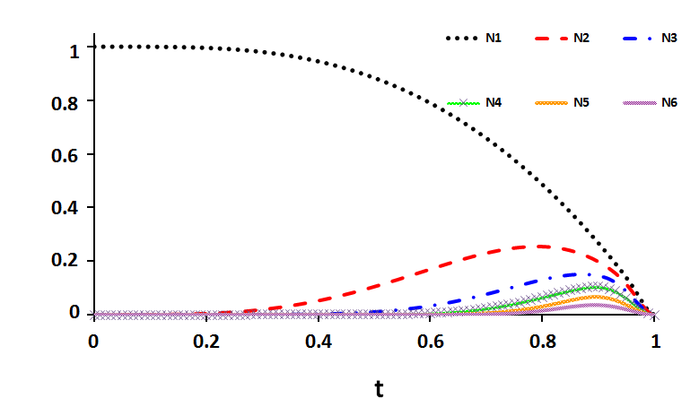
Figure 1: First six eigenvalues of the matrix $D_{\mathrm{even}}$.

Note that $t$ is a very nonlinear parameter: although $t\sim\delta/8k$ for small $\delta$, the value $t=1/2$ means $\mu/\omega=1/9$ or $\delta/k=80/81$. This shows that, unless $\delta$ is pretty close to the dissociation value, the harmonium triplet is not badly described by a Hartree–Fock state. Whenever $t\lesssim 0.6$, that is, $\delta/k\lesssim 255/256$, the first two occupation numbers contain almost all the physical information for the system.

Also, one we can show that whenever $t\lesssim 0.5$, a good approximation to the five first occupation numbers is

$$\lambda_{1}\approx 1-3t^{4}+8t^{6},\quad\lambda_{2}\approx 3t^{4}-8t^{6},\quad\lambda_{3}\approx 5t^{8},\quad\lambda_{4}\approx 7t^{12}\quad\mbox{and}\quad\lambda_{5}\approx 9t^{16}.$$

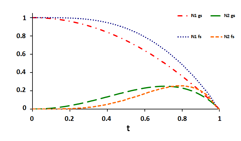
Figure 2: First and second occupation numbers of the ground state and of the first excited state.

Figure 2 compares the behavior of the first two eigenvalues for the singlet and triplet states of harmonium. In this sense, the Hartree–Fock approximation works better in the triplet case than for the singlet. Around $t=0.4$ the second approximated occupation number for the latter is above $0.13$, and for the former is below $0.052$. The same behaviour was also observed in the toy model studied in [43]. This does not mean, however, that correlation is always weaker in the triplet state —see the next section.

8 Spatial entropy and correlation energies

We move towards the comparison of the triplet system with the singlet system in regard to disorder (suppressing the spin variables). To measure this, a useful quantity is the linear entropy $s$ associated to the 1-body function:

$$s=1-\Pi(d_{1}),$$

where $\Pi(d_{1})$ is the purity of the system —see below. Mathematically, the quantity $s$ is a lower bound for the Jaynes entropy, which has been used to quantify the entanglement between one particle and the other $N-1$ particles of the system [43], and proposed as a handle on the correlation energies [44]. In this paper the singlet has been modelled in such a way that, for each one-dimensional mode:

$$\Pi_{\mathrm{gs},1}(d_{1})=\int d_{1}^{2}(r;p)\,dr\,dp=\sum_{i}n_{i}^{2}.$$

Instead, for the triplet one should take for the excited mode:

$$\Pi_{\mathrm{fs},x}(d_{1})=\frac{1}{2}\int d_{1}^{2}(r_{x};p_{x})\,dr_{x}\,dp_{x}=\sum_{i}n_{i}^{2}.$$

This second definition is natural in that correlations due solely to the antisymmetric character of the wave function do not contribute to the entanglement of the system [19, 45, 46]. This ensures that the entropy for a 1-body function of the Hartree–Fock type is zero.

In the singlet case, the occupation numbers are equal to $(1-t^{2})\,t^{2i}$. Thus, the purity of this system is easily computable, to wit, $\Pi_{\mathrm{gs},1}(d_{1})=(1-t^{2})/(1+t^{2})$ for each mode. This quantity coincides with the quotient of the geometric and arithmetic means of the frequencies, that is, $\Pi_{\mathrm{gs},1}=2\sqrt{\omega\mu}/(\omega+\mu)$. For $n$ modes one just takes the $n$th power [18]. Moreover, for small values of the coupling $\delta$, we obtain

$$s_{\mathrm{gs},1}\sim\frac{1}{32}\,\frac{\delta^{2}}{\omega^{4}},$$ (14)

which for this approximation is exactly the absolute value of the (dimensionless) correlation energy [27]. This appears to vindicate the contention of [44]. (Actually, for the singlet it is not difficult to compute the Jaynes entropy, given by

$$-\sum_{i}n_{i}\log n_{i}=-\log(1-t^{2})-\frac{t^{2}\log t^{2}}{1-t^{2}}\,.$$

This was done by Srednicki [21] some time ago.)

For the triplet state, we have to compute $\operatorname{Tr}(d_{1}^{2})$ for the matrix given in (13). Since

$$d_{1}^{2}=(1-t^{2})^{4}\,\begin{pmatrix}1+\alpha^{2}_{0}t^{2}&0&\alpha_{0}t(1+2t^{2}+3t^{4})&\cdots\\ 0&(1+2t^{2})^{2}+\alpha^{2}_{1}t^{6}&0&\cdots\\ \alpha_{0}t(1+2t^{2}+3t^{4})&0&\alpha^{2}_{0}t^{2}+(2t^{2}+3t^{4})^{2}+\alpha^{2}_{2}t^{10}&\cdots\\ \vdots&\vdots&\vdots&\ddots\end{pmatrix},$$

we get

$$\operatorname{Tr}(d_{1}^{2}) =(1-t^{2})^{4}\biggl{[}4\sum_{i=0}^{\infty}\alpha_{i}^{2}\,t^{2(2i+1)}+2\sum_{i=1}^{\infty}i^{2}\,t^{4(i-1)}\biggr{]}$$

$$=2(1-t^{2})^{4}\sum_{i=1}^{\infty}\biggl{[}2i(i+1)\,t^{2(2i-1)}+i^{2}\,t^{4(i-1)}\biggr{]}=\frac{2(1-t^{2})}{1+t^{2}}\biggl{[}1+\frac{2t^{2}}{(1+t^{2})^{2}}\biggr{]},$$

after some calculation. So the purity of the first excited mode is

$$\Pi_{\mathrm{fs},x}=\frac{1-t^{2}}{1+t^{2}}\biggl{[}1+\frac{2t^{2}}{(1+t^{2})^{2}}\biggr{]}=\Pi_{\mathrm{gs},1}\biggl{[}1+\frac{2t^{2}}{(1+t^{2})^{2}}\biggr{]}=\frac{2\sqrt{\omega\mu}}{\omega+\mu}\biggl{(}1+\frac{1}{2}\Bigl{(}\frac{\omega-\mu}{\omega+\mu}\Bigr{)}^{2}\biggr{)}.$$

Since the other two modes contribute with two ground state factors, the total purity can be written as $\Pi_{\mathrm{fs}}=\Pi_{\mathrm{fs},x}\Pi_{\mathrm{gs},y}\Pi_{\mathrm{gs},z}$. For the purity parameter, one obtains finally

$$s_{\mathrm{gs}}=1-\biggl{(}\frac{1-t^{2}}{1+t^{2}}\biggr{)}^{3}\quad\mbox{and}\quad s_{\mathrm{fs}}=1-\biggl{(}\frac{1-t^{2}}{1+t^{2}}\biggr{)}^{3}\biggl{[}1+\frac{2t^{2}}{(1+t^{2})^{2}}\biggr{]}=s_{\mathrm{gs}}-\frac{2t^{2}(1-t^{2})^{3}}{(1+t^{2})^{5}}.$$

In conclusion, $s_{\mathrm{fs}}\leq s_{\mathrm{gs}}$.

At long last, we may go back to Moshinsky’s starting point, the assessment of electron correlation, only now for the excited state. The Hartree–Fock approximation for the relevant mode, in view of (8), is of the form

$$W_{\mathrm{HF}}(r_{1},r_{2};p_{1},p_{2}) =\frac{1}{2}\bigl{[}W_{00}(r_{1};p_{1})W_{11}(r_{2};p_{2})-W_{01}(r_{1};p_{1})W_{10}(r_{2};p_{2})$$

$$\qquad-W_{10}(r_{1};p_{1})W_{01}(r_{2};p_{2})+W_{11}(r_{1};p_{1})W_{00}(r_{2};p_{2})\bigr{]},$$

$$\text{where }W_{00}(r;p) =\frac{1}{\pi}e^{-\eta r^{2}-p^{2}/\eta},\qquad W_{11}(r;p)=\frac{2}{\pi}e^{-\eta r^{2}-p^{2}/\eta}(\eta r^{2}+p^{2}/\eta-\tfrac{1}{2}),$$

with their corresponding interferences. Remember that $\int W_{ij}\,dr\,dp=\delta_{ij}$. In intracule-extracule coordinates:

$$W_{\mathrm{HF}}(R,r;P,p)=\frac{2}{\pi^{2}}\bigl{(}\eta r^{2}+p^{2}/\eta-\tfrac{1}{2}\bigr{)}e^{-\eta R^{2}-P^{2}/\eta-\eta r^{2}-p^{2}/\eta}.$$

The parameter $\eta$ is determined by minimization. The mean value of the energy predicted by this function is:

$$E_{\mathrm{HF}} =\frac{1}{2}\int(p^{2}+\omega^{2}r^{2})[W_{00}(r;p)+W_{11}(r;p)]\,dr\,dp-\frac{\delta}{4}\int(r_{1}-r_{2})^{2}\,W_{\mathrm{HF}}(1,2)\,d1\,d2$$

$$=\biggl{(}\eta+\frac{\omega^{2}}{\eta}\biggr{)}-\frac{3\delta}{4\eta}=\eta+\frac{\omega^{2}+3\mu^{2}}{4\eta}.$$

The minimum $dE/d\eta=0$ occurs when $\eta=\tfrac{1}{2}\sqrt{\omega^{2}+3\mu^{2}}$. Therefore, the energy predicted by Hartree–Fock is $\sqrt{\omega^{2}+3\mu^{2}}$. Thus, the “correlation energy” for the lowest excited state of harmonium is:

$$E_{\mathrm{c},\mathrm{fs}}=E_{\mathrm{fs}}-E_{\mathrm{HF}}=\frac{3\omega+5\mu}{2}-\sqrt{\omega^{2}+3\mu^{2}}-2\sqrt{(\omega^{2}+\mu^{2})/2}\sim-\frac{7}{64}\,\frac{\delta^{2}}{\omega^{3}}\,.$$

Thus, the relative correlation energies are

$$\mathcal{E}_{\mathrm{fs}}:=\frac{|E_{\mathrm{c},\mathrm{fs}}|}{E_{\mathrm{fs}}}\sim\frac{7}{256}\,\frac{\delta^{2}}{\omega^{4}}\quad\mbox{and}\quad\mathcal{E}_{\mathrm{gs}}:=\frac{|E_{\mathrm{c},\mathrm{gs}}|}{E_{\mathrm{gs}}}\sim\frac{1}{32}\,\frac{\delta^{2}}{\omega^{4}}\,.$$

Both quantities are related by a factor of $7/8$. For this approximation, as one would have expected, $\mathcal{E}_{\mathrm{fs}}\leq\mathcal{E}_{\mathrm{gs}}$.

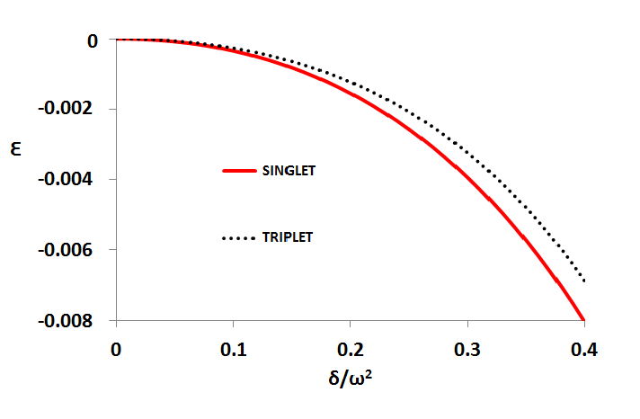
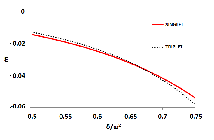
Figure 3: Relative correlation energy of the singlet and of the triplet excited mode. As expected, the relative correlation energy for the singlet is greater than for the triplet for small values of the coupling. At $\delta/\omega^{2}\sim 0.67$ the order is inverted.

Figure 3 shows the exact dependence of the relative correlation energy for both systems as a function of $\delta/\omega^{2}$. The relative correlation energy for the singlet is greater than for the triplet, just as the purity parameter for the singlet is greater than the one for the triplet. At $\delta/\omega^{2}=0.67$ the relation between these two quantities changes and the relative correlation energy for the triplet is greater than for the singlet. Note however that the entropy depends only the behavior of the occupation numbers, while the correlation energy has to do with the natural orbitals as well. Such a nice proportionality as (14) fails for the triplet state.

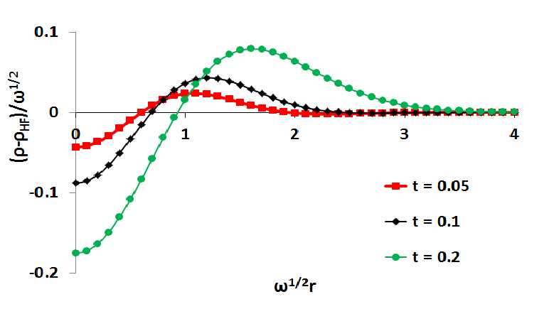
Figure 4: Moshinsky’s hole for the triplet: $(\rho(r)-\rho_{\mathrm{HF}}(r))/\omega^{1/2}$ as a function of $\omega^{1/2}r$.

Finally, Figure 4 shows the difference between the exact profile 1-density and the Hartree–Fock profile 1-density for the harmonium triplet, $\rho_{\mathrm{HF}}(r):=\int W_{\mathrm{HF}}(r,r_{2};p_{1},p_{2})\,dp_{1}\,dr_{2}\,dp_{2}$. This description goes back to the Coulson–Neilson classic paper [47] on the helium Coulomb system. The “Moshinsky’s hole” observed in the neighborhood of $r=0$ graphically shows the Hartree–Fock underestimation of the mean distance between the fermions, for the excited configuration of harmonium as well.

9 Conclusion

From the very beginning of quantum mechanics, the fundamental state of harmonium has provided a useful playground for learning about such questions as correlation energy, entanglement or hole entropy (including black hole entropy). Here, for the first time, we rather exhaustively analyze the (spin triplet) first excited configuration of harmonium, particularly the behaviour of its occupation numbers and natural orbitals. This is a different chemical species altogether, due to the antisymmetric character of the orbital wave function. When exactly reconstructing à la Löwdin–Shull–Kutzelnigg the two-body density as a functional of the one-body density, instead of the sign dilemma (already solved by two of us) for the lowest-energy state, we find, as expected on general grounds, an ambiguity in the choice of natural orbitals.

Also as expected, in the triplet case the first occupation number plays a more dominant role than for the singlet, up to fairly high values of the coupling parameter, $t\lesssim 0.4$. Thus, within this range, modeling the excited configuration as a Hartree–Fock state introduces a lower error than doing so for the ground state. In parallel, the linear entropy of the first excited configuration is lower than that of the ground state, and the relative correlation energy for the excited state stays below that of the ground state for such values of the coupling. The order reverses at higher values of $t$.

Acknowledgments

JMGB thanks the Zentrum für interdisziplinäre Forschung (ZiF) at Bielefeld, in whose welcoming atmosphere this paper received its finishing touches. CMBR and JMGB are grateful to Andrés F. Reyes-Lega for an illuminating discussion. JCV thanks the Departamento de Física Teórica of the Universidad de Zaragoza for warm hospitality.

CLBR and JMGB have been supported by grant FPA2009–09638 of Spain’s central government. CLBR thanks Banco Santander for support. JMGB owes to ZiF for support, as well. JCV acknowledges support from the Dirección General de Investigación e Innovación of Aragon’s regional government, and from the Vicerrectoría de Investigación of the University of Costa Rica.

Last, but not least, we thank the referee for very helpful criticism, questions and suggestions, leading to an improved presentation.

References

• [1]
• [2] W. Heisenberg, Z. Physik 38 411 (1926).
• [3] C. Garrod and J. K. Percus, J. Math. Phys. 105 1756 (1964).
• [4] P. W. Ayers, S. Golden and M. Levy, J. Chem. Phys. 124 054101 (2006).
• [5] D. A. Mazziotti, Chem. Rev. 112 244 (2012).
• [6] D. A. Mazziotti, Phys. Rev. Lett. 108 263002 (2012).
• [7] D. A. Mazziotti, Phys. Rev. A 85 062507 (2012).
• [8] A. M. K. Müller, Phys. Lett. A 105 446 (1984).
• [9] P.-O. Löwdin and H. Shull, Phys. Rev. 101 1730 (1956).
• [10] W. Kutzelnigg, Theor. Chem. Acta 1 327 (1963).
• [11] M. Moshinsky, Am. J. Phys. 36 52 (1968).
• [12] N. H. March, A. Cabo, F. Claro and G. G. N. Angilella, Phys. Rev. A 77 042504 (2008).
• [13] P.-F. Loos, Phys. Rev. A 81 032510 (2010).
• [14] I. Nagy and J. Pipek, Phys. Rev. A 83 034502 (2011).
• [15] C. Amovilli and N. H. March, Phys. Rev. A 67 022509 (2003).
• [16] I. Nagy and J. Pipek, Phys. Rev. A 81 014501 (2010).
• [17] C. Amovilli and N. H. March, Phys. Rev. A 69 054302 (2004).
• [18] J. Pipek and I. Nagy, Phys. Rev. A 79 052501 (2009).
• [19] R. J. Yáñez, A. R. Plastino and J. S. Dehesa, Eur. Phys. J. D 56 141 (2010).
• [20] P. A. Bouvrie, A. P. Majtey, A. R. Plastino, P. Sánchez-Moreno and J. S. Dehesa, Eur. Phys. J. D 66 15 (2012).
• [21] M. Srednicki, Phys. Rev. Lett. 71 666 (1993).
• [22] E. R. Davidson, Reduced Density Matrices in Quantum Chemistry, Academic Press, London, 1976.
• [23] J. M. Gracia-Bondía, Contemp. Math. 134 93 (1992).
• [24] Ph. Blanchard, J. M. Gracia-Bondía and J. C. Várilly, Int. J. Quant. Chem. 112 1134 (2012); physics.chem-ph/1011.4741.
• [25] J. M. Gracia-Bondía and J. C. Várilly, “Exact phase space functional for two-body systems”; physics.chem-ph/1011.4742.
• [26] J. P. Dahl, Can. J. Chem. 87 784 (2009).
• [27] K. Ebrahimi-Fard and J. M. Gracia-Bondía, J. Math. Chem. 50 440 (2012); physics.chem-ph/1103.2023.
• [28] C. L. Benavides-Riveros and J. M. Gracia-Bondía, “Physical Wigner functions”, to appear.
• [29] C. L. Benavides-Riveros and J. C. Várilly, “Testing one-body density functionals on a solvable model”, to appear.
• [30] K. Blum, Density Matrix Theory and Applications, Springer, Berlin, 2012.
• [31] A. Kenfack and K. Życzkowski, J. Opt. B Quant. Semiclass. 6 396 (2004).
• [32] J. P. Dahl, H. Mack, A. Wolf and W. P. Schleich, Phys. Rev. A 74 042323 (2006).
• [33] J. M. Gracia-Bondía and J. C. Várilly, Phys. Lett. A 128 20 (1988).
• [34] A. P. Prudnikov, Yu. A. Brychkov and O. I. Marichev, Integrals and Series, Bell and Bain, Glasgow, 1983.
• [35] G. E. Andrews, R. Askey and R. Roy, Special Functions, Cambridge University Press, Cambridge, 1999.
• [36] A. Knutson and T. Tao, Notices Amer. Math. Soc. 48 175 (2001).
• [37] A. A. Klyachko, J. Phys. Conf. Ser. 36, 72 (2006); quant-ph/0511102.
• [38] A. A. Klyachko, “The Pauli exclusion principle and beyond”, quant-ph/0904.2009.
• [39] J. J. Duistermaat and G. J. Heckman, Invent. Math. 69 259 (1982).
• [40] M. Christandl, B. Doran, S. Kousidis and M. Walter, “Eigenvalue distributions of the reduced density matrices”, quant-ph/1204.0741.
• [41] J. H. Wilkinson, The Algebraic Eigenvalue Problem, Clarendon Press, Oxford 1965.
• [42] E. Lieb, J. Math. Phys. 31 594 (1990).
• [43] N. Helbig, I. V. Tokatly and A. Rubio, Phys. Rev. A 81 022504 (2010).
• [44] G. T. Smith, H. L. Schmider and V. H. Smith, Phys. Rev. A 65 032508 (2002).
• [45] J. Naudts and T. Verhulst, Phys. Rev. A 75 062104 (2007).
• [46] A. P. Balachandran, T. R. Govindarajan, A. R. de Queiroz and A. F. Reyes-Lega, “Entanglement, particle identity and the GNS construction: a unifying approach”, quant-ph/1205.2882.
• [47] C. A. Coulson and A. H. Neilson, Proc. Phys. Soc. 78 831 (1961).