-SUP: A clustering algorithm for cryo-electron microscopy images of asymmetric particles
Abstract
Cryo-electron microscopy (cryo-EM) has recently emerged as a powerful tool for obtaining three-dimensional (3D) structures of biological macromolecules in native states. A minimum cryo-EM image data set for deriving a meaningful reconstruction is comprised of thousands of randomly orientated projections of identical particles photographed with a small number of electrons. The computation of 3D structure from 2D projections requires clustering, which aims to enhance the signal to noise ratio in each view by grouping similarly oriented images. Nevertheless, the prevailing clustering techniques are often compromised by three characteristics of cryo-EM data: high noise content, high dimensionality and large number of clusters. Moreover, since clustering requires registering images of similar orientation into the same pixel coordinates by 2D alignment, it is desired that the clustering algorithm can label misaligned images as outliers. Herein, we introduce a clustering algorithm -SUP to model the data with a -Gaussian mixture and adopt the minimum -divergence for estimation, and then use a self-updating procedure to obtain the numerical solution. We apply -SUP to the cryo-EM images of two benchmark macromolecules, RNA polymerase II and ribosome. In the former case, simulated images were chosen to decouple clustering from alignment to demonstrate -SUP is more robust to misalignment outliers than the existing clustering methods used in the cryo-EM community. In the latter case, the clustering of real cryo-EM data by our -SUP method eliminates noise in many views to reveal true structure features of ribosome at the projection level.
doi:
10.1214/13-AOAS680keywords:
, , , , , , and
1 Introduction and motivating example
Determining 3D atomic structure of large biological molecules is important for elucidating the physicochemical mechanisms underlying vital processes. In 2006, the Nobel Prize in chemistry was awarded to structural biologist Roger D. Kornberg for his studies of the molecular basis of eukaryotic transcription, in which he obtains for the first time an actual picture at the molecular level of the structure of RNA polymerase II during the stage of actively making messenger RNA. Three years later in 2009, the same prize went to three X-ray crystallographers, Venkatraman Ramakrishnan, Thomas A. Steitz and Ada E. Yonath, for their revelation at the atomic level of the structure and workings of the ribosome, with its even larger and more complex machinery that translates the information contained in RNA into a poly-peptide chain. Despite these successes, most large proteins have resisted all attempts at crystallization. This has led to the emergence of cryo-electron microscopy (cryo-EM), an alternative to X-ray crystallography for obtaining 3D structures of macromolecules, since it can focus electrons to form images without the need of crystals [Henderson (1995), van Heel et al. (2000), Saibil (2000), Frank (2002, 2009, 2012, Jiang et al. (2008), Liu et al. (2010), Grassucci, Taylor and Frank (2011)].
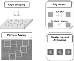
A flowchart for cryo-EM analysis is shown in Figure 1. In the sample preparation step, macromolecules obtained through biochemical purification in the native condition are frozen so rapidly that the surrounding water forms a thin layer of amorphous ice to embed the molecules [Lepault, Booy and Dubochet (1983), Adrian et al. (1984), Dubochet (2012)]. The data obtained by cryo-EM imaging consists of a large number of particle images representing projections from random orientations of the macromolecule. An essential step in reconstructing the 3D structure from these images is to determine the 3D angular relationship of the 2D projections, which is a challenging task for the following reasons. First, the images are of poor quality, as they are heavily contaminated by shot noise induced by the extremely low number of electrons used to prevent radiation damage. Second, in contrast to X-ray crystallography, which restricts the conformation of the macromolecule in the crystal, cryo-EM data retain any conformation variations of the macromolecule that exist in their original solution state, which means the data is a mixture of conformations on top of the viewing angles. The left panel of Figure 1 explains how the 2D cryo-EM images are collected and the right panel shows the commonly used strategy to improve the signal-to-noise ratio (SNR) of those images.
Given reasonably clear 2D projections, an ab initio approach based on the projection-slice theorem for 3D reconstruction from 2D projections is available [Bracewell (1956)]. This theorem states that any two nonparallel 2D projections of the same 3D object would share a common line in Fourier space. This common-line principle underlies the first 3D reconstruction of a spherical virus with icosahedral symmetry from electron microscope micrographs [Crowther et al. (1970)]. The same principle was further applied to the problem of angular reconstruction of the asymmetric particle [van Heel (1987)]. In practice, a satisfactory solution depends on the quality of the images and becomes increasingly unreachable for raw cryo-EM images as the SNR gets too low. It is therefore necessary to enhance the SNR of each view by averaging many well aligned cryo-EM images coming from a similar viewing angle. Clustering is thus aimed at grouping together the cryo-EM images with nearly the same viewing angle. This step requires pre-aligning the images because incorrect in-plane rotations and shiftings would prevent successful clustering. Failure to cluster images into homogeneous groups would, in turn, render the determination of the 3D structure unsatisfactory. Currently, most approaches for clustering cryo-EM images are rooted in the -means method, which has been found to be unsatisfactory [Yang et al. (2012)].
Here, we focus on the clustering step and assume that the image alignment has been carried through. In the vast number of clustering algorithms developed, two major approaches are taken. A model-based approach [Banfield and Raftery (1993)] models the data as a mixture of parametric distributions and the mean estimates are taken to be the cluster centers. A distance-based approach enforces some “distance” to measure the similarity between data points, with notable examples being hierarchical clustering [Hartigan (1975)], the -means algorithm [McQueen (1967), Lloyd (1982)] and the SUP clustering algorithm [Chen and Shiu (2007), Shiu and Chen (2012)]. In this paper, we combine these two approaches to propose a clustering algorithm -SUP. We model the data with a -Gaussian mixture [Amari and Ohara (2011), Eguchi, Komori and Kato (2011)] and adopt the -divergence [Fujisawa and Eguchi (2008), Cichocki and Amari (2010), Eguchi, Komori and Kato (2011)] for measuring the similarity between the empirical distribution and the model distribution, and then borrow the self-updating procedure from SUP [Chen and Shiu (2007), Shiu and Chen (2012)] to obtain a numerical solution. While minimizing the -divergence leads to a soft rejection in the sense that the estimate downweights the deviant points, the -Gaussian mixture helps set a rejection region when the deviation gets too large. Both of these factors resist outliers and contribute robustness to our clustering algorithm. To execute the self-updating procedure, we start with treating each individual data point as the cluster representative of a singleton cluster and, in each iteration, we update the cluster representatives through the derived estimating equations until all the representatives converge. This self-updating procedure ensures that neither knowledge of the number of clusters nor random initial centers are required.
To investigate how -SUP would perform when applied to cryo-EM images, we tested two sets of cryo-EM images. The first set, consisting of noisy simulated RNA polymerase II images of different views projected from a defined orientation, was chosen in order to decouple the alignment issues from clustering issues, allowing for quantitative comparison between -SUP and other clustering methods. The second set consisted of 5000 real cryo-EM images of ribosome bound with an elongation factor that locks it into a defined conformation. For the test on the simulated data, both perfectly aligned cases and misaligned cases were examined. -SUP did well in separating different views in which the images were perfectly aligned and was able to identify most of the deliberately misaligned images as outliers. For the ribosome images, -SUP was successful in that the cluster averages were consistent with the views projected from the known ribosome structure.
The paper is organized as follows. Section 2 reviews the concepts of -divergence and the -Gaussian distribution, which are the core components of -SUP. In Section 3 we develop our -SUP clustering algorithm from the perspective of the minimum -divergence estimation of the -Gaussian mixture model. The performance of -SUP is further evaluated through simulations in Section 4, and through a set of real cryo-EM images in Section 5. The paper ends with a conclusion in Section 6.
2 A review of -divergence and the -Gaussian distribution
In this section we briefly review the concepts of -divergence and the -Gaussian distribution, which are the key technical tools for our -SUP clustering algorithm.
2.1 -divergence
The most widely used divergence of distributions is probably the Kullback-Leibler divergence (KL-divergence) due to its connection to maximum likelihood estimation (MLE). The -divergence, indexed by a power parameter , is a generalization of KL-divergence. Let
where is a nonnegative function defined on . For simplicity, we assume is either a discrete set or a connected region.
Definition 1 ([Fujisawa and Eguchi (2008), Cichocki and Amari (2010), Eguchi, Komori and Kato (2011)]).
For , define the -divergence and -cross entropy as follows:
| (1) | |||
| (2) |
where is a normalizing constant.
The -divergence can be understood as the divergence function associated with a specific scoring function, namely, the pseudospherical score [Good (1971), Gneiting and Raftery (2007)]. The pseudospherical score is given by . The associated divergence function between and can be calculated from equation (7) in Gneiting and Raftery (2007) to be
This implies that and are equivalent. Moreover, can also be expressed as a functional Bregman divergence [Frigyik, Srivastava and Gupta (2008)] by taking . The corresponding Bregman divergence is
where is the Gâteaux derivative of at along direction . Note that is a normalizing constant so that the cross entropy enjoys the property of being projective invariant, that is, , [Eguchi, Komori and Kato (2011)]. By Hölder’s inequality, it can be shown that, for (defined below), and equality holds if and only if for some [Eguchi, Komori and Kato (2011)]. Thus, by fixing a scale, for example,
defines a legitimate divergence on . There are other possible ways of fixing a scale, for example, .
In the limiting case, , which gives the KL-divergence. The MLE, which corresponds to the minimization of the KL-divergence , has been shown to be optimal in parameter estimation in many settings in the sense of having minimum asymptotic variance. This optimality comes with the cost that the MLE relies on the correctness of model specification. Therefore, the MLE or the minimization of the KL-divergence may not be robust against model deviation and outlying data. On the other hand, the minimum -divergence estimation is shown to be robust [Fujisawa and Eguchi (2008)] against data contamination. It is this robustness property that makes -divergence suitable for the estimation of mixture components, where each component is a local model [Mollah et al. (2010)].
2.2 The -Gaussian distribution
The -Gaussian distribution is a generalization of the Gaussian distribution obtained by replacing the usual exponential function with the -exponential
In this article, we adopt , which corresponds to -Gaussian distributions with compact support. We will explain this necessary condition of compact support later.
Let denote the collection of all strictly positive definite symmetric matrices.
Definition 2 ([Modified from Amari and Ohara (2011), Eguchi, Komori and Kato (2011)]).
For a fixed , define the -variate -Gaussian distribution with parameters to have the probability density function (p.d.f.),
| (3) |
where and is a constant so that .
The constant is given below [cf. Eguchi, Komori and Kato (2011)]:
| (4) |
The class of the -Gaussian distributions covers some well-known distributions. In the limit as approaches 1, the -Gaussian distribution reduces to the Gaussian distribution. For , the -Gaussian distribution becomes the multivariate -distribution. This can be seen by setting . Then, in (3) is proportional to
| (5) |
which is exactly the p.d.f. of a -variate -distribution (up to a constant term) with location and scale parameters and degrees of freedom . Depending on the choice of , the support of also differs. For (i.e., for the Gaussian distribution and -distribution), the support of is the entire . For , however, the support of is compact and depends on in the form
| (6) |
Thus, choosing leads to zero mutual influence between clusters in our clustering algorithm. Note that if with ,111For , it ensures the existence of the th moment of . then and .
2.3 Minimum -divergence for estimating a -Gaussian
The -divergence is a discrepancy measure for two functions in . Its minimum can then be used as a criterion to approximate an underlying p.d.f. from a certain model class parameterized by . It has been deduced that minimizing over is equivalent to minimizing the -loss function [Fujisawa and Eguchi (2008)]
| (7) |
Thus, at the population level, is estimated by
| (8) |
At this moment, we consider to be the family of -Gaussian distributions with . Then, for any given values of and , the loss function evaluated at becomes
Direct calculation then gives that minimizing over possible values of is equivalent to maximizing
| (9) |
For high-dimensional data, however, it is impractical to estimate the covariance matrix and its inverse. Since our main interest is to find cluster centers, we employ as our working model. By taking the derivative of (9) with respect to , we get the stationary equation for the maximizer for any fixed :
where is the weight function and is the cumulative distribution function corresponding to .
Given the observed data , the sample analogue of can be obtained naturally by replacing in (2.3) with the empirical distribution function of . This gives the stationarity condition for at the sample level:
| (11) |
One can see that the weight function assigns the contribution of to . Thus, a robust estimator should encourage the property that smaller weight is given to those farther away from and zero weight to extreme outliers. These can be achieved by choosing proper values of in . In particular, when , we have from (6) that
| (12) |
That is, data points outside the range do not have any influence on . Note also that when , then and, thus, in (11) becomes the sample mean , which is not robust to outliers. This fact suggests that we should use a value that is greater than .
3 -SUP
In this section we introduce our clustering method, -SUP, which is derived from minimizing -divergence under a -Gaussian mixture model.
3.1 Model specification and estimation
Suppose we have collected data with empirical probability mass and empirical c.d.f. , where “” is understood componentwise. The goal is to group them into clusters, where is unknown and should be determined from the data. Assume that is a mixture of components with p.d.f.
| (13) |
where each component is modeled by a -Gaussian distribution indexed by . Most model-based clustering approaches (e.g., those assuming a Gaussian mixture model) aim to learn the whole model by minimizing a divergence (e.g., KL-divergence) between and the empirical probability mass . They therefore suffer the problem of having to specify the number of components before implementation. To overcome this difficulty, instead of minimizing to learn directly, we consider learning each component of separately through the minimization problem
| (14) |
The validity of (14) to learning all components of relies on the locality of -divergence, as shown in Lemma 3.1 of Fujisawa and Eguchi (2008). The authors have proven that, at the population level, is approximately proportional to , provided that the model and the remaining components are well separated. We also refer the readers to Mollah et al. (2010) for a comprehensive discussion about the locality of -divergence. Consequently, we are motivated to find all local minimizers of (14), each of which corresponds to an estimate of one component of . Moreover, the number of local minimizers provides an estimate of . A detailed implementation algorithm that finds all local minimizers and estimates is introduced in the next subsection.
3.2 Implementation: Algorithm and tuning parameters
We have shown in Section 2.3 that, for any given , solving (14) is equivalent to finding the cluster center that satisfies the stationary equation (11). Starting with a set of initial cluster centers indexed by , we consider the following fixed-point algorithm to solve (11):
| (15) |
Multiple initial centers are necessary to find multiple solutions of (11). To avoid the problem of random initial centers, in this paper we consider the natural choice
| (16) |
Other choices are possible, but (16) gives a straightforward updating path for each observation . At convergence, the distinct values of provide estimates of the cluster centers and the number of clusters. Moreover, cases whose updating paths converge to the same cluster center are clustered together. Though derived from a minimum -divergence perspective, we note that (15) combined with (16) has the same form as the mean-shift clustering [Fukunaga and Hostetler (1975)] for mode seeking. It turns out that clustering through (15)–(16) shares the same properties as mean-shift clustering. Our -SUP framework provides the mean-shift algorithm an information theoretic justification, namely, it minimizes the -divergence under a -Gaussian mixture model. We call (15)–(16) the “nonblurring -estimator,” to distinguish it from our main proposal introduced in the next paragraph.
While the nonblurring mean-shift updates the cluster centers with the original data points being fixed [which corresponds to a fixed in (15) over iterations], the blurring mean-shift [Cheng (1995)] is a variant of the nonblurring mean-shift algorithm, which updates the cluster centers and moves (i.e., blurs) the data points simultaneously. Shiu and Chen (2012) proposed self-updating process (SUP) as a clustering algorithm. The blurring mean-shift can be viewed as an SUP with a homogeneous updating rule (SUP allows nonhomogeneous updating). It has been reported [Shiu and Chen (2012)] that SUP possesses many advantages, especially in the presence of outliers. Thus, we are motivated to implement the minimum -divergence estimation via an SUP-like algorithm and call it -SUP. In particular, the -SUP algorithm is constructed by replacing in (15) with , to reflect its nature in updating blurred data as model representatives over iterations. That is, after one iteration, we believe that the blurred data is more representative of the population than the previous one and, thus, the blurred data is treated as the new sample to be entered into the next iteration. This gives the self-updating process of -SUP:
| (17) |
The update (17) can be expressed as, for ,
| (18) |
where
with the scale parameter and the model parameter being
| (20) |
Here is a consequence of choosing and as mentioned in the end of Section 2.3. Thus, -SUP involves only as the tuning parameters. It has been found in our numerical studies that -SUP is quite insensitive to the choice of and that plays the decisive role in the performance of -SUP. We thus suggest a choice of a small positive value of , say, 0.025, in practical implementation. A phase transition plot (Figure 5) will be introduced to determine in Section 4.
It can be seen from (18) that, in updating in the th iteration, -SUP takes a weighted average over the candidate model representatives according to the weights . Due to the weights in (3.2) being nonnegative and decreasing with respect to the distance and the compact support of the -Gaussian distribution, the convergence of -SUP is assured [Chen (2013)]. We can express the weights (3.2) as
| (21) |
As a result, -SUP starts with (scaled) cluster centers , which avoids the problem of random initial centers. Eventually, -SUP converges to certain clusters, where depends on the tuning parameters , but otherwise is data-driven. Moreover, we have the cluster representatives , which contain distinct points denoted by . The corresponding cluster membership for each data point is denoted by . The detailed algorithm of -SUP (16)–(17) is summarized in Table 1. Note that in our proposal, we ignore the estimation of . The main reason is that is absorbed into the scale parameter defined in (20), and a phase transition plot can be used to select directly.
| Inputs: Data matrix , instances with variables; |
| Tuning parameters . |
| Outputs: Number of clusters and cluster centers ; |
| Cluster membership assignment for each of . |
| begin |
| start with: , |
| repeat |
| for |
| , |
| end |
| , |
| until convergence |
| output distinct cluster centers } and cluster membership |
| end |
[]Note: The parameter is linearly proportional to the influence region radius that defines the similarity inside a cluster.

A toy example to illustrate how data points move by -SUP is presented in Figure 2. Two clusters with 10 data points each are sampled from the standard normal distributions centered at and , respectively. Another 20 isolated noise points are added surrounding these two clusters. The first plot (upper left) shows the initial positions of these 40 points. Then each data point is updated (blurred) according to the weighted average of its neighboring points. After the th iteration, no (blurred) data points move any more and the algorithm stops. Data points with the same final position are assigned to the same cluster. There are seven clusters at the end of the self-updating process. Two cluster centers are close to the true means of the normal mixture. The other five cluster centers are formed by noise data. Data points sampled from the normal mixture are correctly merged into their target clusters. Some noise points close to these two clusters move into them, while other noise points are merged into five clusters. At the bottom row of Figure 2, we have also provided a plot for comparison with sample means and -means centers. The sample means were computed with the information of the true cluster labels and the -means centers were computed under given , respectively. One can see that, in the presence of outliers, cluster centers from -SUP can still be close to the sample means, while this is not the case for -means under every .
3.3 Characteristics of -SUP
Similar to (18), the nonblurring -estimator (15)–(16) can be expressed as
| (22) |
where . Comparing (18) and (22), the constructed cluster centers from -SUP and the nonblurring -estimator are both weighted averages with the weights and , respectively. The principle of downweighting is important for robust model fitting [Basu et al. (1998), Field and Smith (1994), Windham (1995)]. We emphasize that the downweighting by in (18) is with respect to models, since each cluster center is a weighted average of . On the other hand, downweighting by in (22) is with respect to data, since each cluster center is a weighted average of the original data . The same concept can also be observed in the difference between the nonblurring mean-shift and the blurring mean-shift. It has been shown that the blurring mean-shift has a faster rate of convergence [Carreira-Perpiñán (2006), Chen (2013)]. To our knowledge, however, there is very little statistical evaluation for these two downweighting schemes in the literature. As will be demonstrated in Section 4, from a statistical perspective, downweighting with respect to models is more efficient than with respect to data in estimating the mixture model, which further supports the usage of -SUP in practice.
4 Numerical study
4.1 Synthetic data
We show by simulation that -SUP is more efficient in model parameter estimation than both the nonblurring -estimator and the -means estimator. Random samples of size 100 are generated from a 4-component normal mixture model with p.d.f.
| (23) |
where , , , , and for some . We set and treat as the relevant component of interest, while are noise components. We apply -SUP and the nonblurring -estimator (both with ) and -means to estimate by using the largest cluster center and cluster size fraction as and , respectively. The simulation results with 100 replicates under different values are placed in Figure 3, which includes the MSE of and the mean of plus/minus one standard deviation. To evaluate the sensitivity of each method to the selection of or , we report (the average selected number of components under ) for -SUP and the nonblurring -estimator, and report , the probability of selecting components by the gap-statistic [Tibshirani, Walther and Hastie (2001)], for -means.
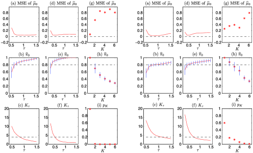
For the case of closely spaced components, where , although -SUP and the nonblurring -estimator perform similarly, -SUP produces smaller MSE in a wider range of values. Moreover, the mean of from -SUP is closer to the target value . On the other hand, -means provides unsatisfactory results for , indicating that -means is sensitive to the selection of when components are not well separated. The superiority of -SUP again has been found in the case of a moderate distance, , among the components. In this situation, -SUP still provides good estimates of over a wide range of , while the selection of becomes more critical for the nonblurring -estimator. The minimum MSE of the nonblurring -estimator happens only around . Since should be determined from the data, this fact supports the applicability of -SUP in practical implementation. The -means algorithm can produce satisfactory results at the true number of components , although its MSE is still the largest among the three methods. However, the gap-statistic does not support the choice of , which increases the difficulty of using a -means with gap-statistic approach for clustering unbalanced-sized components.
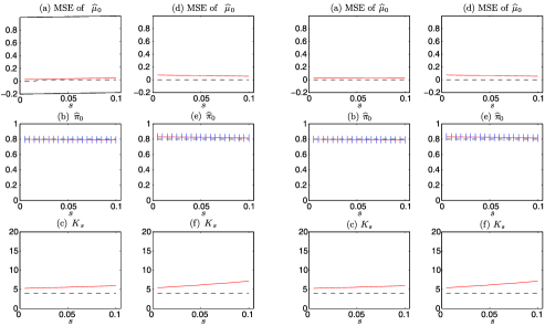
We now evaluate the influence of to -SUP. The same simulation studies with and are conducted. One can see from Figure 4 that the performance of -SUP and the nonblurring -estimator is quite insensitive to the value of and that -SUP is even a bit better, which confirms that the critical tuning parameter is the scale parameter . As to the selection of , one can find an elbow-pattern (or phase transition) of in Figures 3(c) and (f). This phenomenon suggests the necessity of choosing a value of which the number of constructed components becomes stable. It can be seen from Figure 3(a)–(b) and (d)–(e) that the suggested rule corresponds to reasonable performance for -SUP and the nonblurring -estimator, where the best result is still from -SUP. We will further examine this selection criterion in the next study using simulated cryo-EM images. Moreover, as discussed in Section 3.3, -SUP has a faster rate of convergence. Therefore, the computational time of -SUP is shorter than the nonblurring -estimator. In summary, -SUP performs better under different settings and is less sensitive to -selection.
4.2 Simulated cryo-EM images
We use simulated cryo-EM images to demonstrate the superiority of -SUP in clustering homogeneous images while isolating misaligned images. A total of 128 distinct 2D images with pixels were generated by projecting the X-ray crystal structure of RNA polymerase II filtered to 20 Angstroms in equally spaced (angle-wise) orientations.222Data source: The X-ray model of RNA polymerase II is from the Protein Data Bank (PDB: 1WCM). Each image was then convoluted with the electron microscopy contrast transfer function (defocus 2 m). Finally, 6400 images were randomly sampled with replacement from these 128 projections with i.i.d. Gaussian noise added, where , so that the corresponding SNRs are , which reflect the low SNR nature of cryo-EM images. This procedure of simulating cryo-EM images is commonly used in the cryo-EM community [Chang et al. (2010), Singer et al. (2010), Sorzano et al. (2010), Hall, Nogales and Glaeser (2011)]. To reflect the nature of the experiment, we consider two scenarios: {longlist}[1.]
All the images are perfectly aligned.
A portion of the images are misaligned. The misaligned images are treated as outliers and should be identified individually without clustering with other correctly aligned images. Before entering the clustering algorithm, we conducted dimension reduction on this image data set. Instead of using principal component analysis (PCA), we applied multilinear principal component analysis [MPCA, Lu, Plataniotis and Venetsanopoulos (2008), Hung et al. (2012)] to reduce the dimension from to , as MPCA has been shown to be more efficient in dimension reduction for array data such as image sets [Hung et al. (2012)]. The extracted low-dimensional MPCA factor loadings then enter the clustering analysis.
We have tested -SUP, -means, clustering 2D (CL2D) [Sorzano et al. (2010)] and -means+, a variant of the latter two, for comparison. Given a prespecified number of clusters , unlike -means which separates the data into clusters directly, CL2D bisects the clusters iteratively until clusters are constructed. During the clustering process, CL2D dismisses the clusters whose size is below a certain number (30 in our case) and splits the largest cluster into two clusters once a dismiss is executed. Another difference is that CL2D adopts the correntropy [a kernel-based entropy measure, Sorzano et al. (2010)] as the measure of distance, while -means uses the usual Euclidean norm. We thus consider -means+, which is modified from CL2D by using the Euclidean norm instead. Note that CL2D, -means+ and -means require the prespecification of and initial assignments for the cluster centers. CL2D further needs a tuning parameter for the kernel width. We have tried a few kernel widths and picked the best one for CL2D. We present the best results out of 10 runs for CL2D, -means and -means+. In contrast to this, -SUP is deterministic as long as its parameters and are fixed. As has been demonstrated in the previous numerical studies that -SUP is insensitive to the -selection, we fix . We will supply a phase transition diagram in Section 4.2.1 to choose .
To evaluate the performance of each method, we report the impurity and c-impurity numbers as defined below. Let {} be sets of true clusters, {} be sets of constructed clusters, and be the cardinality of the set. For each output cluster , its purity number is defined by . The overall purity number [Manning, Raghavan and Schtze (2008)] is the sum over all output clusters:
The impurity number is defined to be
Note that the purity is usually defined to be the ratio of the purity number and the total number of images. Here we do not normalize it by the total number for better presentation of the simulation results. The impurity number is 0 for the perfect clustering result, but a zero impurity number does not guarantee a perfect clustering. This number cannot recognize mistakes made by splitting one class into two or more clusters. We thus define c-impurity, which is analogous to the impurity number but exchanges the roles of the true clusters and the output clusters to derive its measure of impurity. That is, define
which is able to pick up the mistakes by splitting a cluster into two or more clusters. In summary, small values of the impurity and c-impurity numbers indicate better performance of a clustering method.
4.2.1 Clustering with perfectly-aligned images
Simulation results withperfectly-aligned images are placed in Table 2. For the small noise level of , -SUP, CL2D and -means+ give perfect clustering. For larger values, their clustering accuracies slowly decay as expected, and have comparable performances. CL2D confuses images at an impurity level of (which stands for and ) when . Quite unexpectedly, -means+ confuses images at an impurity level of when but performs flawlessly when . This is due to the 10 random initial centers mentioned above. The performance of -means is poor for all values, even when we correctly specify . This reflects the shortcomings of -means when the noise level is high and when the number of clusters is large.
| -SUP | -SUP | CL2D | -means | -means | |
|---|---|---|---|---|---|
| (SNR0.19) | |||||
| impurity | 0 | 0 | 0 | 0 | 1206 |
| c-impurity | 0 | 0 | 0 | 0 | 425 |
| (SNR0.12) | |||||
| impurity | 44 | 0 | 0 | 34 | 1175 |
| c-impurity | 0 | 0 | 0 | 33 | 462 |
| (SNR0.08) | |||||
| impurity | 150 | 0 | 4 | 0 | 1106 |
| c-impurity | 0 | 0 | 4 | 0 | 465 |
One can see that -SUP has a larger impurity number when , and we found that the errors made by -SUP always involve mistakenly combining two clusters as a single one. In real applications, practitioners are very likely to have prior knowledge about the expected cluster size when analyzing cryo-EM images, and it is common to further bisect an unevenly large cluster. To mimic this situation, we consider -SUP+, which modifies the result of -SUP by further using -means to separate those clusters whose size is greater than 70. This threshold should be adjusted according to the ratio of the total number of images to the number of clusters expected. The results of -SUP+ are also provided in Table 2, where a perfect clustering is achieved for every . This indicates the applicability of our proposal, as an error made by -SUP can be easily fixed. We remind the readers that the true number of components in this simulation is . This makes CL2D (and -means+) beneficial in clustering, since the main idea of CL2D is to bisect data until a prespecified number of clusters is reached. We thus believe using -SUP+ is a fair comparison for our method. We will further see the superiority of -SUP in the presence of outliers (see Section 4.2.2), in which the true number of components largely exceeds , resulting in CL2D becoming less accurate at clustering.
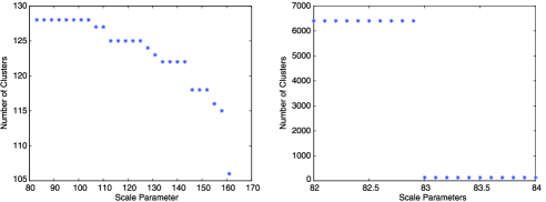
We demonstrate the effect of and provide guidance on its selection. Figure 5 gives the numbers of clusters from -SUP under various values of when , wherein we observe a phase transition in the number of clusters: -SUP outputs 6400 clusters when , outputs 128 clusters (a perfect result) when , and there exists no intermediate result between 128 and 6400. Moreover, the cluster number remains at 128 for quite a wide range of . Recall that the scale parameter is proportional to the support region of the weight (3.2) and, hence, -SUP’s updating procedure ignores the influence of data outside a certain range determined by . When is small enough that there is no influence between any two images, -SUP leads to 6400 clusters (i.e., each individual cryo-EM image forms one cluster). When reaches a critical value, the images in the same cluster can start attracting each other and will finally merge. This explains why a phase transition occurs. We observe similar phase transition phenomena for various noise structures, of which some may not happen at the perfect cluster result, but never happen far from it. Thus, the value at which the phase transition occurs can be treated as a starting value for selecting a reasonable range of .
4.2.2 Clustering with misaligned images
It is well possible that a set of cryo-EM images cannot be well aligned due to their low SNR. A good cluster method should be robust in the presence of misaligned images (outliers). We thus conduct simulations to evaluate the performances of clustering methods, where and of the images are randomly chosen to be rotated by 7.2, 14.4, 21.6, 28.8, 36 or 43.2 angular degrees (∘) clockwise. The effect of this is that each rotated image no longer shares the same signal pattern with the images in its original cluster, nor does it share a signal pattern with the other misaligned ones. An ideal outcome in this scenario would be for the clustering algorithm to treat each of these misaligned images as a singleton cluster. Including these singleton clusters, the total cluster number would become 771 for misalignment and 1410 for , while the meaningful cluster number would remain at 128.
Simulation results are presented in Table 3 for the misalignment scenario and Table 4 for the misalignment scenario. It can be seen that -SUP performs best in comparison with CL2D, -means+ and -means for all values. Moreover, combined with the prior knowledge about expected cluster size, the result from -SUP can be further improved by -SUP+. These outcomes support the applicability of -SUP in the presence of outliers. As shown in Table 3 for the very low SNR case with , -SUP+ has only 7 misaligned images which have been wrongly assigned to true clusters, while the other misaligned images were correctly separated out as outliers. On the other hand, -means+ and CL2D can do nothing about the misaligned images which are () in the misalignment case, such that their default mistakes are 643 in the impurity category. The main reason is that CL2D will still allocate outliers into certain clusters and, hence, the resulting cluster centers will still be subject to the influence of outliers. In contrast, -SUP allows for singleton clusters as indicated in Table 3, and the resulting cluster means are, therefore, more robust.
| -SUP | -SUP | CL2D | -means | -means | |
|---|---|---|---|---|---|
| (SNR0.19) | |||||
| impurity | 0 | 0 | 643 | 789 | 407 |
| c-impurity | 0 | 0 | 0 | 0 | 3452 |
| (SNR0.12) | |||||
| impurity | 83 | 0 | 644 | 788 | 410 |
| c-impurity | 0 | 0 | 1 | 4 | 3482 |
| (SNR0.08) | |||||
| impurity | 190 | 7 | 644 | 779 | 423 |
| c-impurity | 0 | 0 | 1 | 2 | 3541 |
| -SUP | -SUP | CL2D | -means | -means | |
|---|---|---|---|---|---|
| (SNR0.19) | |||||
| impurity | 0 | 0 | 1703 | 1773 | 820 |
| c-impurity | 0 | 0 | 4 | 3 | 3883 |
| (SNR0.12) | |||||
| impurity | 36 | 1 | 1743 | 1760 | 833 |
| c-impurity | 0 | 0 | 1 | 11 | 3899 |
| (SNR0.08) | |||||
| impurity | 214 | 11 | 1726 | 1713 | 824 |
| c-impurity | 0 | 0 | 6 | 1 | 3909 |
The performance of CL2D and -means+ is more seriously impacted when the misaligned proportion is (Table 4). While CL2D makes no other mistake at and makes mistakes at and in addition to the default 643 misalignment images in the case, it makes from 421 to 444 more image merges in addition to the default 1282 () ones for the case. The -means+ method shows similar patterns in both the and the case. This indicates that, as a large number of outliers are forced to enter the clusters, their cluster representatives tend to be contaminated to an extent that it becomes difficult to identify their correct cluster members. In contrast, -SUP provides a solution to this commonly encountered situation.
5 Real cryo-EM image clustering
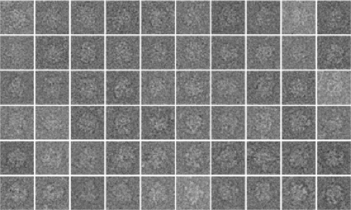
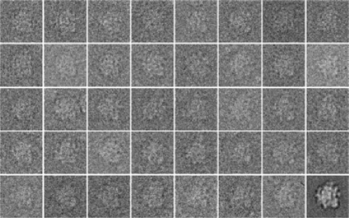
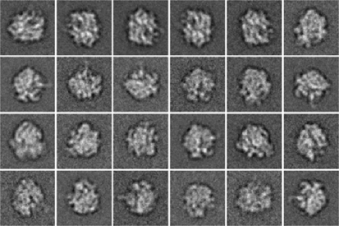
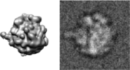
Ribosome is the cellular machinery that synthesizes proteins. The structure of ribosome has been intensively investigated by X-ray crystallography and cryo-EM. For the latter, the structure is obtained by 3D reconstruction using many cryo-EM images. Those images represent projections from different viewing angles. To test the performance of -SUP in grouping experimental data into similar views, a set of E. coli 70s ribosome was downloaded333The website link is http://www.ebi.ac.uk/pdbe/emdb/data/SPIDER_FRANK_data/. (60 sample images are shown in Figure 6). This data set contains 5000 single-particle cryo-EM images of randomly oriented ribosome carrying an elongation factor with it. The 5000 cryo-EM images were preprocessed using XMIPP [Sorzano et al. (2004)] to correct the negative phase component induced by the electron microscope transfer function. Next, the corrected images were centered and roughly aligned using the multi-reference alignment method on the SPIDER suite for single particle processing [Frank et al. (1996)]. The dimension of those images was reduced from to via MPCA [Hung et al. (2012)]. PCA was then further applied to the correlation matrix of those MPCA loading scores. The final dimension of each image is 20. Figure 7 shows a gallery of 39 raw cryo-EM images with a noticeably similar orientation, which were grouped into a single cluster by -SUP using the parameters and , and the average of those images at the right bottom corner, which has clearly brought out an abundance of meaningful detail hidden in the raw images. This particular clustering exemplifies the potential of -SUP in processing real data. A total of 24 clusters with cluster sizes between 23 to 219 were found and their averages are given in Figure 8. We demonstrate their consistency with the 2D projections of known ribosome 3D structure with an example shown in Figure 9. One of the class averages is compared with a 2D projection of a 70s ribosome 3D structure solved by X-ray. The P-stalk [Wilsome and Cate (2012)] with its signature tail on the left side can be clearly seen.
6 Conclusion
We have combined a model-based -Gaussian mixture clustering method, the -estimator and a self-updating process, SUP, to propose -SUP, a novel hybrid designed to meet the image clustering challenges encountered in cryo-EM analysis. Characteristically, sets of cryo-EM images have low SNR, many of which are misaligned and should be treated as outliers, and which form a large number of clusters due to their free orientations. Because of its capability to identify outliers, -SUP can separate out the misaligned images and create the possibility for further correcting them. Thus, we have been able to present a successful application of -SUP on cryo-EM images.
Eliminating the need to set initial random cluster centers and cluster number, -SUP requires only the specification of . We have shown that -SUP has robust performance over in many scenarios. Once is chosen, the phase transition scheme may suggest a reasonable range for . This insensitivity with respect to -selection and the observation of the phase transition greatly reduces the difficulty in selecting the tuning parameters. We summarize the characteristics which make for the success of -SUP:
-
•
-SUP adopts a -Gaussian mixture model with , which has compact support. Hence, it sets a finite influence range for each component and completely rejects data outside this range. When a data point is outside a certain cluster representative’s influence range, it contributes zero weight toward this representative.
-
•
-SUP estimates the model parameters by minimizing -divergence. The minimum -divergence downweights the influence for data that deviates far from the cluster centers, which enhances the clustering robustness.
-
•
-SUP extracts clusters without the need of specifying the number of components and random initial centers. It starts with each individual data point as a singleton cluster [i.e., with a mixture of components, see (16)], and is data-driven.
-
•
-SUP allows singleton or extremely small-sized clusters to accommodate potential outliers.
-
•
-SUP uses to shrink the fitted mixture model toward cluster centers in each iteration. Such a shrinkage acts as if the effective temperature is iteratively decreasing, so that it improves the efficiency of mixture estimation.
Finally, we also remind the readers that the strength of -SUP is for cases where the number of clusters is large, or data are contaminated with noises/outliers, or cluster sizes are not balanced [some clusters are much bigger, or smaller, than others]. However, there is no advantage of using -SUP if the clustering problem arises from normal mixtures whose components have approximately similar sizes.
Acknowledgments
The authors gratefully acknowledge the Editor, the Associate Editor and two reviewers for their comments, which have substantially improved this work. The authors also acknowledge the support from the National Science Council, Taiwan.
References
- Adrian et al. (1984) {barticle}[pbm] \bauthor\bsnmAdrian, \bfnmM.\binitsM., \bauthor\bsnmDubochet, \bfnmJ.\binitsJ., \bauthor\bsnmLepault, \bfnmJ.\binitsJ. and \bauthor\bsnmMcDowall, \bfnmA. W.\binitsA. W. (\byear1984). \btitleCryo-electron microscopy of viruses. \bjournalNature \bvolume308 \bpages32–36. \bidissn=0028-0836, pmid=6322001 \bptokimsref\endbibitem
- Amari and Ohara (2011) {barticle}[mr] \bauthor\bsnmAmari, \bfnmShun-ichi\binitsS.-i. and \bauthor\bsnmOhara, \bfnmAtsumi\binitsA. (\byear2011). \btitleGeometry of -exponential family of probability distributions. \bjournalEntropy \bvolume13 \bpages1170–1185. \biddoi=10.3390/e13061170, issn=1099-4300, mr=2811982 \bptokimsref\endbibitem
- Banfield and Raftery (1993) {barticle}[mr] \bauthor\bsnmBanfield, \bfnmJeffrey D.\binitsJ. D. and \bauthor\bsnmRaftery, \bfnmAdrian E.\binitsA. E. (\byear1993). \btitleModel-based Gaussian and non-Gaussian clustering. \bjournalBiometrics \bvolume49 \bpages803–821. \biddoi=10.2307/2532201, issn=0006-341X, mr=1243494 \bptokimsref\endbibitem
- Basu et al. (1998) {barticle}[mr] \bauthor\bsnmBasu, \bfnmAyanendranath\binitsA., \bauthor\bsnmHarris, \bfnmIan R.\binitsI. R., \bauthor\bsnmHjort, \bfnmNils L.\binitsN. L. and \bauthor\bsnmJones, \bfnmM. C.\binitsM. C. (\byear1998). \btitleRobust and efficient estimation by minimising a density power divergence. \bjournalBiometrika \bvolume85 \bpages549–559. \biddoi=10.1093/biomet/85.3.549, issn=0006-3444, mr=1665873 \bptokimsref\endbibitem
- Bracewell (1956) {barticle}[mr] \bauthor\bsnmBracewell, \bfnmR. N.\binitsR. N. (\byear1956). \btitleStrip integration in radio astronomy. \bjournalAustral. J. Phys. \bvolume9 \bpages198–217. \bidissn=0004-9506, mr=0080017 \bptokimsref\endbibitem
- Carreira-Perpiñán (2006) {bmisc}[auto:STB—2014/01/06—10:16:28] \bauthor\bsnmCarreira-Perpiñán, \bfnmM. A.\binitsM. A. (\byear2006). \bhowpublishedFast nonparametric clustering with Gaussian blurring mean-shift. In Proceeding of the 23rd International Conference on Machine Learning 153–160. ACM, Pittsburgh, PA. \bptokimsref\endbibitem
- Chang et al. (2010) {barticle}[auto:STB—2014/01/06—10:16:28] \bauthor\bsnmChang, \bfnmW.-H.\binitsW.-H., \bauthor\bsnmChiu, \bfnmM.-K.\binitsM.-K., \bauthor\bsnmChen, \bfnmC.-Y.\binitsC.-Y., \bauthor\bsnmYen, \bfnmC.-F.\binitsC.-F., \bauthor\bsnmLin, \bfnmY.-C.\binitsY.-C., \bauthor\bsnmWeng, \bfnmY.-P.\binitsY.-P., \bauthor\bsnmChang, \bfnmJ.-C.\binitsJ.-C., \bauthor\bsnmWu, \bfnmY.-M.\binitsY.-M., \bauthor\bsnmCheng, \bfnmH.\binitsH., \bauthor\bsnmFu, \bfnmJ.\binitsJ. and \bauthor\bsnmTu, \bfnmI.-P.\binitsI.-P. (\byear2010). \btitleZernike phase plate cryo-electron microscopy facilitates single particle analysis of unstained asymmetric protein complexes. \bjournalStructure \bvolume18 \bpages17–27. \bptokimsref\endbibitem
- Chen (2013) {bmisc}[auto:STB—2014/01/06—10:16:28] \bauthor\bsnmChen, \bfnmT.-L.\binitsT.-L. (\byear2013). \bhowpublished On the convergence and consistency of the blurring mean-shift process. Available at \arxivurlarXiv:1305.1040. \bptokimsref\endbibitem
- Chen and Shiu (2007) {bmisc}[auto:STB—2014/01/06—10:16:28] \bauthor\bsnmChen, \bfnmT.-L.\binitsT.-L. and \bauthor\bsnmShiu, \bfnmS.-Y.\binitsS.-Y. (\byear2007). \bhowpublishedA clustering algorithm by self-updating process. In JSM Proceedings, Statistical Computing Section 2034–2038. American Statistical Association, Salt Lake City, UT. \bptokimsref\endbibitem
- Cheng (1995) {barticle}[auto:STB—2014/01/06—10:16:28] \bauthor\bsnmCheng, \bfnmY.\binitsY. (\byear1995). \btitleMean shift, mode seeking, and clustering. \bjournalIEEE Transactions on Pattern Analysis and Machine Intelligence \bvolume17 \bpages790–799. \bptokimsref\endbibitem
- Cichocki and Amari (2010) {barticle}[mr] \bauthor\bsnmCichocki, \bfnmAndrzej\binitsA. and \bauthor\bsnmAmari, \bfnmShun-ichi\binitsS.-i. (\byear2010). \btitleFamilies of alpha- beta- and gamma-divergences: Flexible and robust measures of similarities. \bjournalEntropy \bvolume12 \bpages1532–1568. \biddoi=10.3390/e12061532, issn=1099-4300, mr=2659408 \bptokimsref\endbibitem
- Crowther et al. (1970) {barticle}[pbm] \bauthor\bsnmCrowther, \bfnmR. A.\binitsR. A., \bauthor\bsnmAmos, \bfnmL. A.\binitsL. A., \bauthor\bsnmFinch, \bfnmJ. T.\binitsJ. T., \bauthor\bparticleDe \bsnmRosier, \bfnmD. J.\binitsD. J. and \bauthor\bsnmKlug, \bfnmA.\binitsA. (\byear1970). \btitleThree dimensional reconstructions of spherical viruses by Fourier synthesis from electron micrographs. \bjournalNature \bvolume226 \bpages421–425. \bidissn=0028-0836, pmid=4314822 \bptokimsref\endbibitem
- Dubochet (2012) {barticle}[pbm] \bauthor\bsnmDubochet, \bfnmJ.\binitsJ. (\byear2012). \btitleCryo-EM–the first thirty years. \bjournalJ. Microsc. \bvolume245 \bpages221–224. \bidissn=1365-2818, pmid=22457877 \bptokimsref\endbibitem
- Eguchi, Komori and Kato (2011) {barticle}[mr] \bauthor\bsnmEguchi, \bfnmShinto\binitsS., \bauthor\bsnmKomori, \bfnmOsamu\binitsO. and \bauthor\bsnmKato, \bfnmShogo\binitsS. (\byear2011). \btitleProjective power entropy and maximum Tsallis entropy distributions. \bjournalEntropy \bvolume13 \bpages1746–1764. \biddoi=10.3390/e13101746, issn=1099-4300, mr=2851127 \bptokimsref\endbibitem
- Field and Smith (1994) {barticle}[auto:STB—2014/01/06—10:16:28] \bauthor\bsnmField, \bfnmC.\binitsC. and \bauthor\bsnmSmith, \bfnmB.\binitsB. (\byear1994). \btitleRobust estimation: A weighted maximum likelihood approach. \bjournalInternational Statistical Review \bvolume62 \bpages405–424. \bptokimsref\endbibitem
- Frank (2002) {barticle}[pbm] \bauthor\bsnmFrank, \bfnmJoachim\binitsJ. (\byear2002). \btitleSingle-particle imaging of macromolecules by cryo-electron microscopy. \bjournalAnnu. Rev. Biophys. Biomol. Struct. \bvolume31 \bpages303–319. \biddoi=10.1146/annurev.biophys.31.082901.134202, issn=1056-8700, pii=082901.134202, pmid=11988472 \bptokimsref\endbibitem
- Frank (2009) {barticle}[pbm] \bauthor\bsnmFrank, \bfnmJoachim\binitsJ. (\byear2009). \btitleSingle-particle reconstruction of biological macromolecules in electron microscopy—30 years. \bjournalQ. Rev. Biophys. \bvolume42 \bpages139–158. \biddoi=10.1017/S0033583509990059, issn=1469-8994, mid=NIHMS180050, pii=S0033583509990059, pmcid=2844734, pmid=20025794 \bptokimsref\endbibitem
- Frank (2012) {barticle}[pbm] \bauthor\bsnmFrank, \bfnmJoachim\binitsJ. (\byear2012). \btitleIntermediate states during mRNA-tRNA translocation. \bjournalCurr. Opin. Struct. Biol. \bvolume22 \bpages778–785. \biddoi=10.1016/j.sbi.2012.08.001, issn=1879-033X, mid=NIHMS399764, pii=S0959-440X(12)00131-5, pmcid=3508672, pmid=22906732 \bptokimsref\endbibitem
- Frank et al. (1996) {barticle}[auto:STB—2014/01/06—10:16:28] \bauthor\bsnmFrank, \bfnmJ.\binitsJ., \bauthor\bsnmRadermachera, \bfnmM.\binitsM., \bauthor\bsnmPenczeka, \bfnmP.\binitsP., \bauthor\bsnmZhua, \bfnmJ.\binitsJ., \bauthor\bsnmLi, \bfnmY.\binitsY., \bauthor\bsnmLadjadj, \bfnmM.\binitsM. and \bauthor\bsnmLeitha, \bfnmA.\binitsA. (\byear1996). \btitleSPIDER and WEB: Processing and visualization of images in 3D electron microscopy and related fields. \bjournalJournal of Structural Biology \bvolume116 \bpages190–199. \bptokimsref\endbibitem
- Frigyik, Srivastava and Gupta (2008) {barticle}[mr] \bauthor\bsnmFrigyik, \bfnmBéla A.\binitsB. A., \bauthor\bsnmSrivastava, \bfnmSantosh\binitsS. and \bauthor\bsnmGupta, \bfnmMaya R.\binitsM. R. (\byear2008). \btitleFunctional Bregman divergence and Bayesian estimation of distributions. \bjournalIEEE Trans. Inform. Theory \bvolume54 \bpages5130–5139. \biddoi=10.1109/TIT.2008.929943, issn=0018-9448, mr=2589887 \bptokimsref\endbibitem
- Fujisawa and Eguchi (2008) {barticle}[mr] \bauthor\bsnmFujisawa, \bfnmHironori\binitsH. and \bauthor\bsnmEguchi, \bfnmShinto\binitsS. (\byear2008). \btitleRobust parameter estimation with a small bias against heavy contamination. \bjournalJ. Multivariate Anal. \bvolume99 \bpages2053–2081. \biddoi=10.1016/j.jmva.2008.02.004, issn=0047-259X, mr=2466551 \bptokimsref\endbibitem
- Fukunaga and Hostetler (1975) {barticle}[mr] \bauthor\bsnmFukunaga, \bfnmKeinosuke\binitsK. and \bauthor\bsnmHostetler, \bfnmLarry D.\binitsL. D. (\byear1975). \btitleThe estimation of the gradient of a density function, with applications in pattern recognition. \bjournalIEEE Trans. Inform. Theory \bvolumeIT-21 \bpages32–40. \bidissn=0018-9448, mr=0388638 \bptokimsref\endbibitem
- Gneiting and Raftery (2007) {barticle}[mr] \bauthor\bsnmGneiting, \bfnmTilmann\binitsT. and \bauthor\bsnmRaftery, \bfnmAdrian E.\binitsA. E. (\byear2007). \btitleStrictly proper scoring rules, prediction, and estimation. \bjournalJ. Amer. Statist. Assoc. \bvolume102 \bpages359–378. \biddoi=10.1198/016214506000001437, issn=0162-1459, mr=2345548 \bptokimsref\endbibitem
- Good (1971) {bmisc}[auto:STB—2014/01/06—10:16:28] \bauthor\bsnmGood, \bfnmI. J.\binitsI. J. (\byear1971). \bhowpublishedComment on “Measuring information and uncertainty.” In Foundation of Statistical Inference (V. P. Godambe and D. A. Sprott, eds.) 265–273. Holt, Rinehart and Winston, Toronto. \bptokimsref\endbibitem
- Grassucci, Taylor and Frank (2011) {barticle}[auto:STB—2014/01/06—10:16:28] \bauthor\bsnmGrassucci, \bfnmR.\binitsR., \bauthor\bsnmTaylor, \bfnmD.\binitsD. and \bauthor\bsnmFrank, \bfnmJ.\binitsJ. (\byear2011). \btitlePreparation of macromolecular complexes for cryo-electron microscopy. \bjournalNature Protocols \bvolume2 \bpages3239–3246. \bptokimsref\endbibitem
- Hall, Nogales and Glaeser (2011) {barticle}[pbm] \bauthor\bsnmHall, \bfnmR. J.\binitsR. J., \bauthor\bsnmNogales, \bfnmE.\binitsE. and \bauthor\bsnmGlaeser, \bfnmR. M.\binitsR. M. (\byear2011). \btitleAccurate modeling of single-particle cryo-EM images quantitates the benefits expected from using Zernike phase contrast. \bjournalJ. Struct. Biol. \bvolume174 \bpages468–475. \biddoi=10.1016/j.jsb.2011.03.020, issn=1095-8657, mid=NIHMS298611, pii=S1047-8477(11)00085-2, pmcid=3138492, pmid=21463690 \bptokimsref\endbibitem
- Hartigan (1975) {bbook}[mr] \bauthor\bsnmHartigan, \bfnmJohn A.\binitsJ. A. (\byear1975). \btitleClustering Algorithms. \bpublisherWiley, \blocationNew York. \bidmr=0405726 \bptokimsref\endbibitem
- Henderson (1995) {barticle}[pbm] \bauthor\bsnmHenderson, \bfnmR.\binitsR. (\byear1995). \btitleThe potential and limitations of neutrons, electrons and X-rays for atomic resolution microscopy of unstained biological molecules. \bjournalQ. Rev. Biophys. \bvolume28 \bpages171–193. \bidissn=0033-5835, pmid=7568675 \bptokimsref\endbibitem
- Hung et al. (2012) {barticle}[mr] \bauthor\bsnmHung, \bfnmHung\binitsH., \bauthor\bsnmWu, \bfnmPeishien\binitsP., \bauthor\bsnmTu, \bfnmIping\binitsI. and \bauthor\bsnmHuang, \bfnmSuyun\binitsS. (\byear2012). \btitleOn multilinear principal component analysis of order-two tensors. \bjournalBiometrika \bvolume99 \bpages569–583. \biddoi=10.1093/biomet/ass019, issn=0006-3444, mr=2966770 \bptokimsref\endbibitem
- Jiang et al. (2008) {barticle}[pbm] \bauthor\bsnmJiang, \bfnmWen\binitsW., \bauthor\bsnmBaker, \bfnmMatthew L.\binitsM. L., \bauthor\bsnmJakana, \bfnmJoanita\binitsJ., \bauthor\bsnmWeigele, \bfnmPeter R.\binitsP. R., \bauthor\bsnmKing, \bfnmJonathan\binitsJ. and \bauthor\bsnmChiu, \bfnmWah\binitsW. (\byear2008). \btitleBackbone structure of the infectious epsilon15 virus capsid revealed by electron cryomicroscopy. \bjournalNature \bvolume451 \bpages1130–1134. \biddoi=10.1038/nature06665, issn=1476-4687, pii=nature06665, pmid=18305544 \bptokimsref\endbibitem
- Lepault, Booy and Dubochet (1983) {barticle}[pbm] \bauthor\bsnmLepault, \bfnmJ.\binitsJ., \bauthor\bsnmBooy, \bfnmF. P.\binitsF. P. and \bauthor\bsnmDubochet, \bfnmJ.\binitsJ. (\byear1983). \btitleElectron microscopy of frozen biological suspensions. \bjournalJ. Microsc. \bvolume129 \bpages89–102. \bidissn=0022-2720, pmid=6186816 \bptokimsref\endbibitem
- Liu et al. (2010) {barticle}[pbm] \bauthor\bsnmLiu, \bfnmHongrong\binitsH., \bauthor\bsnmJin, \bfnmLei\binitsL., \bauthor\bsnmKoh, \bfnmSok Boon S.\binitsS. B. S., \bauthor\bsnmAtanasov, \bfnmIvo\binitsI., \bauthor\bsnmSchein, \bfnmStan\binitsS., \bauthor\bsnmWu, \bfnmLily\binitsL. and \bauthor\bsnmZhou, \bfnmZ. Hong\binitsZ. H. (\byear2010). \btitleAtomic structure of human adenovirus by cryo-EM reveals interactions among protein networks. \bjournalScience \bvolume329 \bpages1038–1043. \biddoi=10.1126/science.1187433, issn=1095-9203, mid=NIHMS392370, pii=329/5995/1038, pmcid=3412078, pmid=20798312 \bptokimsref\endbibitem
- Lloyd (1982) {barticle}[mr] \bauthor\bsnmLloyd, \bfnmStuart P.\binitsS. P. (\byear1982). \btitleLeast squares quantization in PCM. \bjournalIEEE Trans. Inform. Theory \bvolume28 \bpages129–137. \biddoi=10.1109/TIT.1982.1056489, issn=0018-9448, mr=0651807 \bptokimsref\endbibitem
- Lu, Plataniotis and Venetsanopoulos (2008) {barticle}[pbm] \bauthor\bsnmLu, \bfnmHaiping\binitsH., \bauthor\bsnmPlataniotis, \bfnmKonstantinos N. Kostas\binitsK. N. K. and \bauthor\bsnmVenetsanopoulos, \bfnmAnastasios N.\binitsA. N. (\byear2008). \btitleMPCA: Multilinear principal component analysis of tensor objects. \bjournalIEEE Trans. Neural. Netw. \bvolume19 \bpages18–39. \biddoi=10.1109/TNN.2007.901277, issn=1045-9227, pmid=18269936 \bptokimsref\endbibitem
- Manning, Raghavan and Schtze (2008) {bbook}[auto:STB—2014/01/06—10:16:28] \bauthor\bsnmManning, \bfnmC.\binitsC., \bauthor\bsnmRaghavan, \bfnmP.\binitsP. and \bauthor\bsnmSchtze, \bfnmH.\binitsH. (\byear2008). \btitleIntroduction to Information Retrieval. \bpublisherCambridge Univ. Press, \blocationNew York. \bptokimsref\endbibitem
- McQueen (1967) {bmisc}[auto:STB—2014/01/06—10:16:28] \bauthor\bsnmMcQueen, \bfnmJ.\binitsJ. (\byear1967). \bhowpublishedSome methods for classification and analysis of multivariate observations. In Proceedings of the Fifth Berkeley Symposium on Mathematical Statistics and Probability 291–297. Univ. California Press, Berkeley, CA. \bptokimsref\endbibitem
- Mollah et al. (2010) {barticle}[auto:STB—2014/01/06—10:16:28] \bauthor\bsnmMollah, \bfnmM. N. H.\binitsM. N. H., \bauthor\bsnmSultana, \bfnmN.\binitsN., \bauthor\bsnmMinami, \bfnmM.\binitsM. and \bauthor\bsnmEguchi, \bfnmS.\binitsS. (\byear2010). \btitleRobust extraction of local structures by the minimum beta-divergence method. \bjournalNeural Networks \bvolume23 \bpages226–238. \bptokimsref\endbibitem
- Saibil (2000) {barticle}[auto:STB—2014/01/06—10:16:28] \bauthor\bsnmSaibil, \bfnmH. R.\binitsH. R. (\byear2000). \btitleMacromolecular structure determination by cryo-electron microscopy. \bjournalActa Crystallographica Section D-Biological Crystallography \bvolume56 \bpages1215–1222. \bptokimsref\endbibitem
- Shiu and Chen (2012) {bmisc}[auto:STB—2014/01/06—10:16:28] \bauthor\bsnmShiu, \bfnmS.-Y.\binitsS.-Y. and \bauthor\bsnmChen, \bfnmT.-L.\binitsT.-L. (\byear2012). \bhowpublishedClustering by self-updating process. Available at \arxivurlarXiv:1201.1979. \bptokimsref\endbibitem
- Singer et al. (2010) {barticle}[pbm] \bauthor\bsnmSinger, \bfnmAmit\binitsA., \bauthor\bsnmCoifman, \bfnmRonald R.\binitsR. R., \bauthor\bsnmSigworth, \bfnmFred J.\binitsF. J., \bauthor\bsnmChester, \bfnmDavid W.\binitsD. W. and \bauthor\bsnmShkolnisky, \bfnmYoel\binitsY. (\byear2010). \btitleDetecting consistent common lines in cryo-EM by voting. \bjournalJ. Struct. Biol. \bvolume169 \bpages312–322. \biddoi=10.1016/j.jsb.2009.11.003, issn=1095-8657, mid=NIHMS167041, pii=S1047-8477(09)00306-2, pmcid=2826584, pmid=19925867 \bptokimsref\endbibitem
- Sorzano et al. (2004) {barticle}[pbm] \bauthor\bsnmSorzano, \bfnmC. O. S.\binitsC. O. S., \bauthor\bsnmMarabini, \bfnmR.\binitsR., \bauthor\bsnmVelázquez-Muriel, \bfnmJ.\binitsJ., \bauthor\bsnmBilbao-Castro, \bfnmJ. R.\binitsJ. R., \bauthor\bsnmScheres, \bfnmS. H W.\binitsS. H. W., \bauthor\bsnmCarazo, \bfnmJ. M.\binitsJ. M. and \bauthor\bsnmPascual-Montano, \bfnmA.\binitsA. (\byear2004). \btitleXMIPP: A new generation of an open-source image processing package for electron microscopy. \bjournalJ. Struct. Biol. \bvolume148 \bpages194–204. \biddoi=10.1016/j.jsb.2004.06.006, issn=1047-8477, pii=S1047-8477(04)00126-1, pmid=15477099 \bptokimsref\endbibitem
- Sorzano et al. (2010) {barticle}[auto:STB—2014/01/06—10:16:28] \bauthor\bsnmSorzano, \bfnmC. O. S.\binitsC. O. S., \bauthor\bsnmBilbao-Castro, \bfnmJ. R.\binitsJ. R., \bauthor\bsnmShkolnisky, \bfnmY.\binitsY., \bauthor\bsnmAlcorlo, \bfnmM.\binitsM., \bauthor\bsnmMelero, \bfnmR.\binitsR., \bauthor\bsnmCaffarena-Fernandez, \bfnmG.\binitsG., \bauthor\bsnmLi, \bfnmM.\binitsM., \bauthor\bsnmXu, \bfnmG.\binitsG., \bauthor\bsnmMarabini, \bfnmR.\binitsR. and \bauthor\bsnmCarazo, \bfnmJ. M.\binitsJ. M. (\byear2010). \btitleA clustering approach to multireference alignment of single-particle projections in electron microscopy. \bjournalJournal of Structural Biology \bvolume171 \bpages197–206. \bptokimsref\endbibitem
- Tibshirani, Walther and Hastie (2001) {barticle}[mr] \bauthor\bsnmTibshirani, \bfnmRobert\binitsR., \bauthor\bsnmWalther, \bfnmGuenther\binitsG. and \bauthor\bsnmHastie, \bfnmTrevor\binitsT. (\byear2001). \btitleEstimating the number of clusters in a data set via the gap statistic. \bjournalJ. R. Stat. Soc. Ser. B Stat. Methodol. \bvolume63 \bpages411–423. \biddoi=10.1111/1467-9868.00293, issn=1369-7412, mr=1841503 \bptokimsref\endbibitem
- van Heel (1987) {barticle}[auto:STB—2014/01/06—10:16:28] \bauthor\bparticlevan \bsnmHeel, \bfnmM.\binitsM. (\byear1987). \btitleAngular reconstitution: A posteriori assignment of projection directions for 3D reconstruction. \bjournalUltramicroscopy \bvolume21 \bpages111–124. \bptokimsref\endbibitem
- van Heel et al. (2000) {barticle}[pbm] \bauthor\bparticlevan \bsnmHeel, \bfnmM.\binitsM., \bauthor\bsnmGowen, \bfnmB.\binitsB., \bauthor\bsnmMatadeen, \bfnmR.\binitsR., \bauthor\bsnmOrlova, \bfnmE. V.\binitsE. V., \bauthor\bsnmFinn, \bfnmR.\binitsR., \bauthor\bsnmPape, \bfnmT.\binitsT., \bauthor\bsnmCohen, \bfnmD.\binitsD., \bauthor\bsnmStark, \bfnmH.\binitsH., \bauthor\bsnmSchmidt, \bfnmR.\binitsR., \bauthor\bsnmSchatz, \bfnmM.\binitsM. and \bauthor\bsnmPatwardhan, \bfnmA.\binitsA. (\byear2000). \btitleSingle-particle electron cryo-microscopy: Towards atomic resolution. \bjournalQ. Rev. Biophys. \bvolume33 \bpages307–369. \bidissn=0033-5835, pmid=11233408 \bptokimsref\endbibitem
- Wilsome and Cate (2012) {barticle}[auto:STB—2014/01/06—10:16:28] \bauthor\bsnmWilsome, \bfnmD.\binitsD. and \bauthor\bsnmCate, \bfnmJ.\binitsJ. (\byear2012). \btitleThe structure and function of the eukaryotic ribosome. \bjournalCold Spring Harbor Perspectives in Biology \bvolume4 \bpagesa011536. \bptokimsref\endbibitem
- Windham (1995) {barticle}[mr] \bauthor\bsnmWindham, \bfnmMichael P.\binitsM. P. (\byear1995). \btitleRobustifying model fitting. \bjournalJ. R. Stat. Soc. Ser. B Stat. Methodol. \bvolume57 \bpages599–609. \bidissn=0035-9246, mr=1341326 \bptokimsref\endbibitem
- Yang et al. (2012) {barticle}[pbm] \bauthor\bsnmYang, \bfnmZhengfan\binitsZ., \bauthor\bsnmFang, \bfnmJia\binitsJ., \bauthor\bsnmChittuluru, \bfnmJohnathan\binitsJ., \bauthor\bsnmAsturias, \bfnmFrancisco J.\binitsF. J. and \bauthor\bsnmPenczek, \bfnmPawel A.\binitsP. A. (\byear2012). \btitleIterative stable alignment and clustering of 2D transmission electron microscope images. \bjournalStructure \bvolume20 \bpages237–247. \biddoi=10.1016/j.str.2011.12.007, issn=1878-4186, mid=NIHMS347568, pii=S0969-2126(11)00467-9, pmcid=3426367, pmid=22325773 \bptokimsref\endbibitem