Detectability of cold streams into high-redshift galaxies by absorption lines

Tobias Goerdt¹, Avishai Dekel², Amiel Sternberg³, Orly Gnat² and Daniel Ceverino¹

¹Departamento de Física Teórica, Universidad Autónoma de Madrid, 28049 Madrid, España
²Racah Institute of Physics, The Hebrew University, Jerusalem 91904, Israel
³The Raymond and Beverly Sackler School of Physics and Astronomy, Tel Aviv University, Tel Aviv 69978, Israel tobias.goerdt@uam.esdekel@phys.huji.ac.ilamiel@wise.tau.ac.ilorlig@phys.huji.ac.ildaniel.ceverino@uam.es

(Draft version )

Abstract

Cold gas streaming along the dark-matter filaments of the cosmic web is predicted to be the major provider of resources for disc buildup, violent disk instability and star formation in massive galaxies in the early universe. We study to what extent these cold streams are traceable in the extended circum-galactic environment of galaxies via ${\rm Ly}\alpha$ absorption and selected low ionisation metal absorption lines. We model the expected absorption signatures using high resolution zoom-in AMR cosmological simulations. In the postprocessing, we distinguish between self-shielded gas and unshielded gas. In the self-shielded gas, which is optically thick to Lyman continuum radiation, we assume pure collisional ionisation for species with an ionisation potential greater than 13.6 eV. In the optically thin, unshielded gas these species are also photoionised by the meta-galactic radiation. In addition to absorption of radiation from background quasars, we compute the absorption line profiles of radiation emitted by the galaxy at the centre of the same halo. We predict the strength of the absorption signal for individual galaxies without stacking. We find that the ${\rm Ly}\alpha$ absorption profiles produced by the streams are consistent with observations of absorption and emission ${\rm Ly}\alpha$ profiles in high redshift galaxies. Due to the low metallicities in the streams, and their low covering factors, the metal absorption features are weak and difficult to detect.

keywords:

cosmology: theory — galaxies: evolution — galaxies: formation — galaxies: high redshift — intergalactic medium — galaxies: ISM

^†^†pagerange: Detectability of cold streams into high-redshift galaxies by absorption lines–References^†^†pubyear: 2012

1 Introduction

Cold gas is thought to flow into massive haloes $\sim 10^{12}M_{\odot}$ at $z=2-3$ along filaments with velocities of $\lower 2.15277pt\hbox{$\;\buildrel>\over{\sim}\;$}200\,{\rm km\,s^{-1}}$ . This phenomenon is predicted by simulations and theoretical analysis, where high-z massive galaxies are continuously fed by narrow, cold, intense, partly clumpy, gaseous streams that penetrate through the shock-heated halo gas into the inner galaxy (Birnboim & Dekel, 2003; Keres et al., 2005; Dekel & Birnboim, 2006; Ocvirk, Pichon & Teyssier, 2008; Keres et al., 2009; Dekel et al., 2009; Johansson, Naab & Ostriker, 2009). They form a dense, unstable, turbulent disc with a bulge and trigger rapid star formation (Dekel, Sari & Ceverino, 2009; Agertz, Teyssier & Moore, 2009; Ceverino, Dekel & Bournaud, 2010; Krumholz & Burkert, 2010; Agertz, Teyssier & Moore, 2011; Ceverino et al., 2012; Cacciato, Dekel & Genel, 2012; Genel, Dekel & Cacciato, 2012; Genzel et al., 2011). N-body simulations suggest that about half the mass in dark-matter halos is built-up smoothly, suggesting that the baryons are also accreted semi-continuously as the galaxies grow (Genel et al., 2010). Indeed, hydrodynamical cosmological simulations reveal that the rather smooth gas components, including mini-minor mergers with mass ratio smaller than 1:10, brings in about two thirds of the mass (Dekel et al., 2009). The massive, clumpy and star-forming discs observed at $z\sim 2$ (Genzel et al., 2008; Genel et al., 2008; Förster Schreiber et al., 2009, 2011) may have been formed primarily via the smooth and steady accretion provided by the cold streams, with a smaller contribution by major merger events (Agertz, Teyssier & Moore, 2011; Ceverino, Dekel & Bournaud, 2010).

Pettini et al. (2002); Adelberger et al. (2003); Shapley et al. (2003) explored the kinematics of the intergalactic medium in the early universe in great dept using high-resolution spectroscopy. Steidel et al. (1996) proposed that the predicted inflowing gas could show up as redshifted metal absorption lines in the spectra of Lyman-break galaxies (LBGs). However, it seems that only a small fraction of the LBGs exhibit redshifted absorption features, which was interpreted as an indication for the absence of cold streams in haloes with $4\times 10^{11}<M_{\rm v}<10^{12}M_{\odot}$ (Steidel et al., 2010, hereafter S10). This has to be reconciled with the robust theoretical prediction that the predicted filaments are ubiquitous in haloes in the early universe. The goal of our paper is to predict the absorption-line signatures of the cold flows, for a detailed comparison with observations like S10.

Goerdt et al. (2010) used cosmological hydrodynamical AMR simulations to predict the characteristics of ${\rm Ly}\alpha$ emission from the cold gas streams. The ${\rm Ly}\alpha$ luminosity in their simulations is powered by the release of gravitational energy as the gas is flowing with a rather constant velocity down the potential gradient toward the halo centre. The simulated ${\rm Ly}\alpha$ -blobs (LABs) are similar in many ways to the observed LABs. Some of the observed LABs may thus be regarded as direct detections of the cold streams that drove galaxy evolution at high $z$ . Observations seem to support this picture (Rauch et al., 2011; Erb, Bogosavljević & Steidel, 2011). On the other hand, Faucher-Giguere et al. (2010), using SPH simulations, predict lower ${\rm Ly}\alpha$ luminosities than Goerdt et al. (2010), and find it difficult to explain the observed LAB luminosities with inflow-driven cooling radiation alone. This is partly because Faucher-Giguere et al. (2010) exclude emission from very dense gas, and partly because the SPH simulations underestimate the energy dissipation of the inflowing gas as it interacts with itself and with the hot medium. They make the point that the gas temperature should also be taken into account when distinguishing between the optically thin and thick regimes. New AMR simulations incorporating radiative transfer seem to confirm the Goerdt et al. (2010) model (Rosdahl & Blaizot, 2012; Kasen et al., in preparation). In particular, Kasen et al. (in preparation) analysing high-resolution cosmological AMR-hydro simulations with full radiative transport for the ionising radiation from background and from stars and for the ${\rm Ly}\alpha$ scattering find that about half the spatially extended ${\rm Ly}\alpha$ luminosity originates from fluorescence due to ionising radiation from new stars, and the other half from cooling emission due to the gravitational energy gain, yielding a total luminosity that is comparable to the findings of Goerdt et al. (2010) based on crude approximations for the radiative transport and without the fluorescence. In a pioneering observation, Cantalupo, Lilly & Haehnelt (2012) detected extended ${\rm Ly}\alpha$ emission from circum-galactic filaments of cold gas that seem to largely arise from fluorescence excited by the UV radiation from an AGN. They detected dark galaxies and circum-galactic filaments that are fluorescently illuminated by a quasar. The properties of these ${\rm Ly}\alpha$ sources all indicate that the sample is consistent with having much of the ${\rm Ly}\alpha$ emission originating in fluorescent reprocessing of quasar radiation.

Bertone & Schaye (2012) investigated the nature and detectability of redshifted rest-frame UV line emission from the IGM at $2<z<5$ . They used simulations to create maps of a set of strong rest-frame UV emission lines. They conclude that several species (e.g., C III, C IV, Si III, Si IV, and O VI) of those from the high-redshift IGM will become detectable in the near future. They also claim that lower ionisation lines provide us with tools to image cold accretion flows as well as cold outflowing clouds.

Refer to caption — Figure 1: Gas density in a simulated galaxy (resolution $70\,{\rm pc}$ ) at $z=2.3$ with $M_{\rm v}=3.5\times 10^{11}M_{\odot}$ . The colour refers to the maximum density along the line of sight. The contours mark $n=0.1$ , 0.01 and $0.001\,{\rm cm}^{-3}$ , respectively. The circle shows the virial radius which is 74 kpc. The inflow is dominated by three cold narrow streams that are partly clumpy. The density in the streams is $n=0.003-0.1\,{\rm cm}^{-3}$ , with the clump cores reaching $n\sim 1\,{\rm cm}^{-3}$ . The white open boxes tag main features such as streams. The same type of points is used to identify these features in figure 3.

Van de Voort et al. (2012), using SPH simulations, find that nearly all of the H i absorption arises in gas that has remained fairly cold, at least while it was extragalactic. In addition, the majority of the H i is rapidly falling towards a nearby galaxy, with non-negligible contributions from outflowing and static gas. They identify carefully the environment of the H i absorbers and conclude with this information that cold accretion flows are critical for the success of simulations in reproducing the observed rate of incidence of damped ${\rm Ly}\alpha$ and particularly that of Lyman limit systems. They propose that cold accretion flows exist and have already been detected in the form of high column density H i absorbers.

\psfrag{XHI}[B][B][1][0]{$X_{\rm HI}$}\psfrag{nHcm-3}[B][B][1][0]{$n_{\rm H}$ [cm${}^{-3}$]}\psfrag{UVX}[Bl][Bl][1][0]{UVX}\psfrag{UVX + local sources}[Bl][Bl][1][0]{UVX + local sources}\psfrag{radiative transfer}[Bl][Bl][1][0]{radiative transfer}\psfrag{shielded/thin}[Bl][Bl][1][0]{shielded/thin}\psfrag{density criterion}[Bl][Bl][1][0]{density criterion}\psfrag{(this paper)}[Bl][Bl][1][0]{(this paper)}\includegraphics[width=173.27718pt]{micheletest13A.eps}

Figure 2: Distribution by volume of the neutral hydrogen fractions

x_{\rm HI}

and total hydrogen gas densities

n_{\rm H}

in the circumgalactic environment of our simulated galaxy (see text). The left panel shows the distributions for the full radiative transfer calculation including the metagalactic UVX field plus internal sources presented by F11. The middle panel is for the radiative transfer calculation, but with UVX only. The right panel are results employing a pure density criterion of

n_{\rm H,shield}=0.01

cm^-3 for the boundary between self-shielded and optically thin cells. The units of the colour-bar axis are unity per unit area in the (log

{}_{10}\,X_{\rm HI}

, log

{}_{10}\,n_{\rm H}

) plane. Contour lines are at 0.0001, 0.001 and 0.01 respectively. Our simplified ionisation model provides a useful crude approximation for the UVX radiative transfer results (see text).

Kacprzak et al. (2010) analysed synthetic Mg ii absorption spectra from simulated galaxies at $z=1$ and they tentatively concluded that most of the Mg ii absorption arises in filaments and tidal streams of the galactic halo. This material is infalling with velocities around 200 km s^-1. They claim that large equivalent-width (EW) Mg ii are associated with outflows.

Faucher-Giguere & Keres (2011), Kimm et al. (2011), Stewart et al. (2011) and Fumagalli et al. (2011, hereafter F11) estimated from simulations the covering factor of the cold streams at $z=2-4$ for absorption from a background source. They found that it is small and decreasing with time. Stewart et al. (2011) and F11 argue that as a galaxy switches from cold- to hot-mode accretion with decreasing redshift the reduced cold gas accretion naturally results in a suppression of cool circumgalactic gas. This transition occurs when the halo is massive enough to support a stable shock near the virial radius (Birnboim & Dekel, 2003; Keres et al., 2005; Dekel & Birnboim, 2006). F11 discover that within $\sim$ 500 Myr of reaching this threshold mass, the covering fraction drops. Because the cold-stream covering factor is small compared to the order unity covering fraction expected for galactic winds, the cold streams are generally overwhelmed by outflows in absorption spectra. However, F11 show that there is enough cross section in the cold flows that could make them detectable in ${\rm Ly}\alpha$ absorption in surveys of background sources. Note the differences with the observations of galaxies at zero impact parameter, i.e. observations in the transverse direction, using e.g. quasars. Van de Voort et al. (2012) and F11 show that in fact there is a significant contribution to the population of absorption line systems that comes from the streams. That is, outflows are prominent, but inflows should be visible as well.

Kimm et al. (2011) and F11 investigated whether the cold gas streams are expected to be detectable in low-ionisation metal absorption lines, such as C ii (1334 Å) or Si ii (1260 Å). They find that the metal absorption signal by the interstellar medium of the central galaxy itself is so deep and so broad in velocity space that it swamps the metal signal from the filamentary gas, which is rather metal poor. A cold filament might be detectable in metal lines if it lies precisely along the line-of-sight, but this would be rare.

Shen et al. (2012) used SPH simulations adopting a blastwave scheme for supernova feedback which, in combination with a high gas density threshold for star formation, has been shown to generate large-scale galactic outflows. Their strong outflows avoid the incoming dense narrow streams, and find their way out in a wide solid angle through the dilute medium between the streams. Showing that the cold inflows are not affected by the outflows. They generate synthetic spectra by drawing sightlines through the simulated CGM at different galactocentric impact parameters, and compared the theoretical interstellar absorption line strengths with the observations. They find that they are in broad agreement with those observed at high-redshift by S10.

As in the observations of S10, we consider separately absorption features of radiation emitted from background sources and from central sources, namely along lines of sight with finite and with vanishing impact parameter with respect to the galaxy at the centre of the halo that hosts the absorbing gas. A theoretical study of absorption in the central-source geometry has not been attempted so far. The same is true for a statistical study of absorption signal in individual galaxies without stacking. We focus on predicting absorption line profiles that correspond to the measurements of S10. We refer to the same ten different lines and mimic their observational procedure by averaging data for several simulated galaxies and many lines of sight. As in F11, we employ high-resolution AMR simulations that are described in Ceverino, Dekel & Bournaud (2010). The spatial resolution in these simulations is 20 times better than in the Horizon MareNostrum simulation (Ocvirk, Pichon & Teyssier, 2008) used by Kimm et al. (2011, they also used higher resolution simulations for verification purposes). Unlike in F11, we do not employ a full radiative transport analysis, and instead account for self-shielding by a simple density criterion that approximates the radiative-transport results. The computations include explicitly highly ionised species (e.g. C iv) created in the warm highly ionised intergalactic medium (as opposed to C ii and others that are created in the cold low-ionised neutral medium).

Our paper is organised as follows. In section 2 we introduce the simulations used for this analysis. In section 3 we explain the computation of the absorption features. In section 4 we show the results for the central geometry. In section 5 we show the results for the background geometry. Finally, in section 6 we draw our conclusions.

2 The Simulations

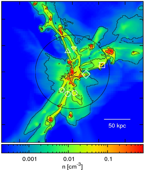
We use three simulated galaxies from a suite of simulations, employing Eulerian adaptive mesh refinement (AMR) hydrodynamics in a cosmological setting. These are zoom-in simulations in dark-matter haloes with masses $\sim 5\times 10^{11}M_{\odot}$ at $z=2.3$ , with a maximum resolution of $35-70\,{\rm pc}$ in physical coordinates (Ceverino, Dekel & Bournaud, 2010, hereafter CDB). Figure 1 shows a density map of one of the three galaxies from the simulation, which serves as our fiducial galaxy. It demonstrates the dominance of typically three co-planar narrow cold streams (see Danovich et al., 2012), originating outside the virial radius along the dark-matter filaments of the cosmic web, penetrating into the discs at the halo centres. The streams consist of a smooth component and clumps with a spectrum of sizes. The typical densities in the streams are in the range $n=0.003-0.1\,{\rm cm}^{-3}$ , and they reach $n=1\,{\rm cm}^{-3}$ near the central disk and at the clump centres. Some of those clumps are satellites with dark matter haloes.

The CDB simulations were run with the art (adaptive refinement tree; Kravtsov, Klypin & Khokhlov, 1997; Kravtsov, 2003) code. It incorporates relevant physical processes for galaxy formation, including gas cooling, photo-ionisation, heating, star formation, metal enrichment and stellar feedback (Ceverino & Klypin, 2009). Cooling rates were computed for the given gas density, temperature, metallicity and UV background (based on cloudy, Ferland et al., 1998). Cooling is assumed at the centre of a cloud of uniform density with thickness 1 kpc (Ceverino-Rodriguez, 2008; Robertson & Kravtsov, 2008). Metallicity dependent, metal-line cooling is included, assuming a relative abundance of elements equal to the solar composition. The code implements a “constant” feedback model, in which the combined energy from stellar winds and supernova explosions is released as a constant heating rate over 40 Myr. This is the typical age of the lightest star that explodes as a type-II supernova. Photo-heating is also taken into account self-consistently with radiative cooling. A uniform UV background based on the Haardt & Madau (1996) model is assumed. Local sources are ignored.

This code has a unique feature for the purpose of simulating the detailed structure of the streams and the gravitational instability in the disk. It allows gas cooling to well below $10^{4}$ K. This enables high densities in pressure equilibrium with the hotter and more dilute medium. A non-thermal pressure floor has been implemented to ensure that the Jeans length is resolved by at least seven resolution elements preventing artificial fragmentation on the smallest grid scale (Truelove et al., 1997; Robertson & Kravtsov, 2008; Ceverino, Dekel & Bournaud, 2010). The pressure floor is effective in the dense $(n>10$ cm ${}^{-3})$ and cold $(T<10^{4}K)$ regions inside galactic disks. Most of the absorbing gas in question, which is far outside the disk, is not affected by this pressure floor.

The equation of state remains unchanged at all densities. Stars form in cells where the gas temperature is below $10^{4}$ K and its density is above the threshold $n=1\,{\rm cm}^{-3}$ according to a stochastic model that is roughly consistent with the Kennicutt (1998) law. The ISM is enriched by metals from supernovae type II and type Ia. Metals are released from each stellar particle by SNII at a constant rate for 40 Myr since its birth. A Miller & Scalo (1979) IMF is assumed. This procedure matches the results of Woosley & Weaver (1995). The metal ejection by SNIa assumes an exponentially declining SNIa rate from a maximum at 1 Gyr. The code treats the advection of metals self-consistently and it distinguishes between SNII and SNIa ejecta (Ceverino-Rodriguez, 2008).

\psfrag{fc(>N)}[B][B][1][0]{$f_{\rm c}(>N_{\rm HI})$}\psfrag{Ncm2}[B][B][1][0]{$N_{\rm HI}$ [cm${}^{-2}$]}\psfrag{HI}[B][B][1][0]{H\,{i}}\psfrag{cg}[Bl][Bl][1][0]{central source}\psfrag{visibility limit}[Bl][Bl][1][0]{visibility limit}\psfrag{ze138me138e12}[Br][Br][1][0]{{\color[rgb]{1,0,0}$z=1.4\,M_{\rm v}=1.4\times 10^{12}\,$M${}_{\odot}$}}\psfrag{ze233me35e11}[Br][Br][1][0]{{\color[rgb]{0,0,1}$z=2.3\,M_{\rm v}=3.5\times 10^{11}\,$M${}_{\odot}$}}\includegraphics[width=240.42569pt]{XXcovfrac03e.eps}

Figure 4: Cumulative

{\rm Ly}\alpha

sky covering fractions

f_{\rm c}

higher than column density

N_{\rm HI}

. It is integrated from 0.3 to 1.0

R_{\rm v}

for all gas inflowing and outflowing. For the blue dashed line we use our three simulated galaxies (resolution

70\,{\rm pc}

) at

z=2.3

with

M_{\rm v}=3.5\times 10^{11}M_{\odot}

and

R_{\rm v}=74\,

kpc, for the red solid line we use two simulated galaxies at

z=1.38

with

M_{\rm v}=1.38\times 10^{12}M_{\odot}

and

R_{\rm v}=150\,

kpc. The observational visibility limit at 10

{}^{13}\,

cm^-2 is indicated by the vertical line. We see very low

(<0.3)

covering fraction over almost the whole range of column densities and a a sharp jump of the covering fraction at the visibility limit. The higher redshift galaxy has a considerably higher covering fraction over the whole range of column densities.

The dark matter particle mass is $5.5\times 10^{5}M_{\odot}$ . The minimum star particle mass is $10^{4}M_{\odot}$ . The initial conditions for the CDB simulations were created using a low-resolution cosmological $N$ -body simulation in a co-moving box of side 29 Mpc. Its cosmological parameters were motivated by WMAP5 (Komatsu et al., 2009). The values are: $\Omega_{\rm m}=0.27$ , $\Omega_{\Lambda}=0.73$ , $\Omega_{\rm b}=0.045$ , $h=0.7$ and $\sigma_{8}=0.82$ . At $z=1$ , three haloes of $M_{\rm v}\simeq 10^{12}M_{\odot}$ each have been selected, avoiding haloes that were subject to a major merger at that time. The three halo masses at $z=2.3$ are $3.5,4,6\times 10^{11}M_{\odot}$ , their virial radii are around 74 kpc and they end up as $(3-4)\times 10^{12}$ M_⊙ haloes today. Around each halo, a concentric sphere of radius twice the virial radius was selected for resimulation with high resolution. Gas was added to the box following the dark matter distribution with a fraction $f_{\rm b}=0.15$ . The whole box was then re-simulated, with refined resolution only in the selected volume about the respective galaxy.

\psfrag{fc(>N)}[B][B][1][0]{$f_{\rm c}(>N_{\rm Ai})$}\psfrag{Ncm2}[B][B][1][0]{$N_{\rm Ai}$ [cm${}^{-2}$]}\psfrag{CII}[B][B][1][0]{{\color[rgb]{1,0,0}C\,{ii}}}\psfrag{CIV}[B][B][1][0]{{\color[rgb]{0,1,0}C\,{iv}}}\psfrag{OI}[B][B][1][0]{{\color[rgb]{0,0,1}O\,{i}}}\psfrag{SiII}[B][B][1][0]{{\color[rgb]{1,0,1}Si\,{ii}}}\psfrag{SiIV}[B][B][1][0]{{\color[rgb]{0,1,1}Si\,{iv}}}\psfrag{MgII}[B][B][1][0]{{\color[rgb]{1,1,0}Mg\,{ii}}}\psfrag{FeII}[B][B][1][0]{{\color[rgb]{0,0,0}Fe\,{ii}}}\psfrag{OII}[B][B][1][0]{{\color[rgb]{0,0,0}O\,{ii}}}\psfrag{OIII}[B][B][1][0]{{\color[rgb]{0,0,0}O\,{iii}}}\psfrag{cg}[Bl][Bl][1][0]{central source}\psfrag{visibility limit}[Br][Br][1][0]{visibility limit}\psfrag{ze138}[Bl][Bl][1][0]{$z=1.4$}\psfrag{ze233}[Bl][Bl][1][0]{$z=2.3$}\psfrag{me1.38e12}[Bl][Bl][1][0]{$M_{\rm v}=1.4\times 10^{12}$ M${}_{\odot}$}\psfrag{me3.5e11}[Bl][Bl][1][0]{$M_{\rm v}=3.5\times 10^{11}$ M${}_{\odot}$}\includegraphics[width=262.90361pt]{XXcovfrac03f.eps}

Figure 5: Same cumulative sky covering fractions as in figure 4 this time for metal lines. In the right panel we use our three simulated galaxies (resolution

70\,{\rm pc}

z=2.3

M_{\rm v}=3.5\times 10^{11}M_{\odot}

and

R_{\rm v}=74\,

kpc), in the left panel we use two simulated galaxies at

z=1.38

with

M_{\rm v}=1.38\times 10^{12}M_{\odot}

and

R_{\rm v}=150\,

kpc. The observational visibility limit at 10

{}^{13}\,

cm^-2 is indicated by the vertical line. Together with figure 4 this plot shows that a full sky map of column densities exhibits a few very high peaks corresponding to the streams extending only over a fairly tiny solid angle and a majority of very low column density solid angle corresponding to the space without streams. This effect is stronger for the low redshift panels.

3 Computing the ionisation states

A reliable estimate of the ionisation state of the gas is essential for any study of absorption line systems. Ideally, the determination of the ionisation states of the gas should be coupled to the hydrodynamic calculations, but due to the numerical complexity of the problem this type of calculation remains computationally expensive for high resolution simulations especially at lower redshifts. In order to compute them via post-processing we take the densities, temperatures and metallicities from the simulation. We assume a primordial helium mass fraction $Y=0.24$ , corresponding to a helium particle abundance of $1/12$ relative to hydrogen. For the heavy elements we assume the Asplund et al. (2009) solar photosphere pattern.

We determine whether a given simulation cell is “self-shielded”, i.e. optically thick to Lyman continuum radiation, via a simple density criterion. Cells with total hydrogen exceeding $n_{\rm shield}\equiv 0.01$ cm^-3 are assumed to be self-shielded. For lower densities the cells are assumed to be optically thin. We find that setting $n_{\rm shield}=0.01$ cm^-3 gives the best agreement with a radiative transfer calculation as we demonstrate in figure 2 (see discussion below). For a further discussion of the density criterion, see the discussion by Cox (2005) or the appendix A2 of F11. We calculate the atomic and ionic fractions $x_{\rm Ai}$ using cloudy (Ferland et al., 1998), where $x_{\rm Ai}$ is defined as the fractions of element $A$ in ionisation state $i$ . The specific species we are interested in are H i, O i, C ii, C iv, Si ii and Si iv. These are the most important ions that are visible and detected in optical spectra at $z=2-3$ and discussed in great detail by S10. We also consider Mg ii and Fe ii since they are assumed to be very suitable for future observational programmes. Table 1 lists the wavelengths and oscillator strengths of the various absorption lines we consider.

ion	$\lambda_{0}$ [Å]	$f_{\lambda}$	$\gamma_{\lambda}$ [s^-1]
${\rm Ly}\alpha$	1215.6701	0.4164	$6.265\times 10^{8}$
C ii	1334.5323	0.1278	$2.870\times 10^{8}$
Si ii	1260.4221	1.115	$2.533\times 10^{9}$
O i	1302.1685	0.04887	$5.750\times 10^{8}$
Si ii	1526.7066	0.1155	$1.960\times 10^{9}$
Si ii	1304.3702	0.09345	$1.720\times 10^{9}$
C iv	1548.195	0.1908	$2.654\times 10^{8}$
Si iv	1393.755	0.514	$8.825\times 10^{8}$
C iv	1550.770	0.09522	$2.641\times 10^{8}$
Si iv	1402.770	0.2553	$8.656\times 10^{8}$
Mg ii	2796.352	0.6123	$2.612\times 10^{8}$
Fe ii	2382.765	0.3006	$3.100\times 10^{8}$

Table 1: Basic parameters of the various absorption lines, we quote wavelength

\lambda_{0}

, oscillator strength

f_{\lambda}

and the damping width

\gamma_{\lambda}

which is the sum over the spontaneous emission coefficients. Data is taken from Morton (1991), except for the

f_{\lambda}

-values for the three Si ii lines, which are from Dufton et al. (1983).

\psfrag{relative intensity}[B][B][1][0]{relative intensity}\psfrag{cg}[Bl][Bl][1][0]{central source}\psfrag{corrfig}[Bl][Bl][1][0]{see figure \ref{fig:ewhammer}}\psfrag{vks}[B][B][1][0]{$\Delta w$ [km s${}^{-1}$]}\psfrag{D}[B][B][1][0]{D}\psfrag{W0=0.064A}[Bl][Bl][1][0]{$W_{0}=0.064$ \AA}\psfrag{W0=0.055A}[Bl][Bl][1][0]{$W_{0}=0.055$ \AA}\psfrag{W0=0.10A}[Bl][Bl][1][0]{$W_{0}=0.10$ \AA}\psfrag{W0=0.056A}[Bl][Bl][1][0]{$W_{0}=0.056$ \AA}\psfrag{NCII=1.2e14}[Bl][Bl][1][0]{$N_{\rm CII}=1.2\times 10^{14}$ cm${}^{-2}$}\psfrag{NSiII=1.5e13}[Bl][Bl][1][0]{$N_{\rm SiII}=1.5\times 10^{13}$ cm${}^{-2}$}\psfrag{NMgII=1.0e13}[Bl][Bl][1][0]{$N_{\rm MgII}=1.0\times 10^{13}$ cm${}^{-2}$}\psfrag{NFeII=1.2e13}[Bl][Bl][1][0]{$N_{\rm FeII}=1.2\times 10^{13}$ cm${}^{-2}$}\psfrag{CII}[Bl][Bl][1][0]{{C\,{ii}} (1334 \AA)}\psfrag{SiIIb}[Bl][Bl][1][0]{{Si\,{ii}} (1260 \AA)}\psfrag{MgIIb}[Bl][Bl][1][0]{{Mg\,{ii}} (2796 \AA)}\psfrag{FeIIb}[Bl][Bl][1][0]{{Fe\,{ii}} (2383 \AA)}\includegraphics[width=140.55667pt]{XXline25voigtz04b02.eps}

Figure 7: Same figure as figure 6, panel D (the panel with the deepest signal) this time for selected metal lines providing also the deepest signal, namely: C ii (1334 Å), Si ii (1260 Å), Mg ii (2796 Å) and Fe ii (2383 Å). Panel D is fully saturated in

{\rm Ly}\alpha

but still shows peak absorption line depths of 0.2 and EW of

\sim 0.1

Å for these metal lines. The C ii panel of this plot disagrees with the results of Kimm et al. (2011, their figure 2, lower panel) due to different line computing algorithms.

In our cloudy computations we distinguish between self-shielded and optically thin cells as follows. For optically thin cells, we assume that the gas is exposed to the full Haardt & Madau (1996) UV to X-ray (UVX) metagalactic background field at the appropriate redshift. We do not include any radiation from “local sources”. The ionisation state is then controlled by the combined effects of electron-impact collisional ionisation and photoionisation for the full spectral range of the background field. For shielded cells, we truncate the radiation field and include only photons with energies below the Lyman limit. Hydrogen and other species with ionisation potentials (IP) greater than 13.6 eV are then produced by collisional ionisation only¹¹1The reader should note that all our species listed in Table 1 have IPs greater than 13.6 eV.. For the shielded cells we neglect photoionisation by penetrating X-rays. So for pure collisional ionisation in shielded cells the hydrogen becomes ionised for $T\lower 2.15277pt\hbox{$\;\buildrel>\over{\sim}\;$}2\times 10^{4}$ K (Gnat & Sternberg, 2007). However, “low-ions” with IPs below 13.6 eV continue to be produced by photoionisation as well. Thus, for a given cell, the ionisation state is determined by its total hydrogen density $n_{\rm H}$ and temperature $T$ , and the adopted radiation field, which is either the “full” or “truncated” Haardt & Madau (1996) field, depending on whether the cell is characterised as shielded or not.

To verify our procedure for distinguishing between shielded and optically thin cells, we compare our results for the hydrogen ionisation states with the more detailed radiative transfer computations presented by F11. In figure 2 we plot the distributions by volume of the neutral hydrogen fractions $x_{\rm HI}$ and total hydrogen gas densities $n_{\rm H}$ in the simulation cells, for three different computations of the ionisation structure, all for the same simulated galaxy. The left-hand panel shows the neutral fraction versus density distributions for the detailed radiative transfer computation of F11. This includes the combined effects of the external UVX and internal sources of photoionising radiation. The middle panel shows the F11 results for UVX only. Cells with densities higher than 0.1 cm^-3, which usually are close to the disc or the satellites, are not included in figure 2. The right-hand panel shows our results for $x_{\rm HI}$ versus $n_{\rm H}$ using our simple criterion of assuming the cells are fully shielded for $n_{\rm H}>n_{{\rm H,shield}}=0.01$ cm^-3. Again, in the post-processing we assume that the hydrogen is collisionally ionised in the shielded cells, and collisionally plus photoionised in the optically thin cells. It is apparent that this simplified model provides a useful crude approximation for the results of the UVX radiative transfer (middle panel). The only significant disparity occurs near the transition density of 0.01 cm^-3 and neutral fraction of $x_{\rm HI}\approx 0.1$ , where the ionisation states appear to be sensitive to the details of the radiative transfer computations. At the end of section 5 we will compare our “final product” (figures 24 and 25) to similar results already published in the literature computed with full radiative transfer including ionising radiation from local sources (figure 13 of F11). The differences are small, justifying our simplifying model.

4 Central source

In this section we consider the ${\rm Ly}\alpha$ and metal line absorption that occurs as UV light emitted by the central galaxy is absorbed by gas in the circum-galactic environment. As defined by S10, the circumgalactic medium is situated in the spherical zone from just outside the galactic disk to around the virial radius $R_{\rm v}$ . Observations of absorption against the central galaxy itself have the advantage of being able to discriminate between inflows and outflows because the absorptions may be assumed to occur in foreground material only. Radiation emitted or scattered from behind the galaxy is blocked by the galaxy itself. However, such absorptions do not provide spatial information about the distance from the galaxy centre as they are all by definition at an impact parameter $b=0$ from the galaxy centre. S10 employed this technique of observing absorptions against the central galaxy by stacking a sample of 89 galaxies with $z=2.3\pm 0.3$ using both rest-frame far-UV and H $\alpha$ spectra, to investigate the kinematics of the gas flows in the circumgalactic regions. Here we predict the spectral line profiles and equivalent widths (=EW) produced in absorption against the central galaxy, for a direct comparison to the S10 observations (as presented in their section 4).

The absorption-line profiles depend on the column densities along the line-of-sight. We compute the column densities along radial rays from an innermost radius $r_{\rm i}$ (usually around the galactic disk) to the virial radius $R_{\rm v}$ . The column $N_{\rm Ai}(\phi,\theta)$ of element $A$ in ionisation state $i$ , at angular position $(\phi,\theta)$ is calculated by

N_{\rm Ai}(\phi,\theta)=\int^{\rm R_{\rm v}}_{\rm r_{i}}x_{\rm Ai}(\vec{r})\ n_{\rm A}(\vec{r})\ dr,

(1)

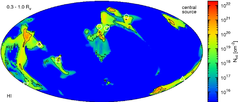
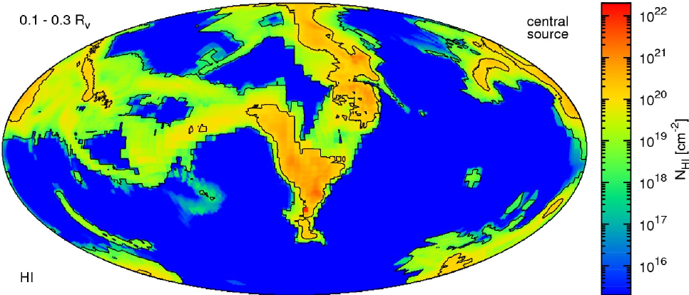
where $n_{\rm A}(\vec{r})$ is the total gas density of element $A$ at position $\vec{r}=(\phi,\theta,r)$ and $x_{\rm Ai}$ is the ionisation fraction. In figure 3 we show two Hammer equal area projections (Snyder, 1993) of H i column densities for our fiducial galaxy ( $z=2.3$ , $M_{\rm v}=3.5\times 10^{11}M_{\odot}$ , $R_{\rm v}=74$ kpc). In the upper panel the column densities are integrated from 0.3 to 1.0 $R_{\rm v}$ whereas in the lower panel they are integrated from 0.1 to 0.3 $R_{\rm v}$ . Excluding the very inner sphere is somewhat artificial since in practise absorption will occur from close to the very centre at $r=0$ . However, these plots are useful in giving an impression of the distribution of column densities along different sight-lines. In the upper panel the main stream features are identified and tagged to the same features shown in figure 1 by white open symbols. The same symbols types in figures 1 and 3 indicate identical features in the galaxy but for different geometries. In figure 3 the narrow major streams with column densities up to $\sim 10^{22}$ cm^-2 can be seen, as well as the vast majority of the “stream-free” sky (as seen from the central galaxy) having only column densities of $<10^{15}$ cm^-2.

To quantify the column density distribution, we compute the cumulative fraction $f_{\rm c}$ of the sky (as viewed from the central galaxy) that is covered with column densities greater than $N_{\rm Ai}$ . The covering fractions for hydrogen and the various metal ions are plotted in figures 4 and 5. These plots include inflowing and outflowing gas. The data in the blue dashed line of figure 4 as well as in the right panel of figure 5 is averaged over our three simulated galaxies at $z=2.3$ with $M_{\rm v}=3.5\times 10^{11}M_{\odot}$ . For better comparability with future observations we also use a second set of data consisting of two galaxies at $z=1.38$ with $M_{\rm v}=1.4\times 10^{12}M_{\odot}$ (red, solid line). The plot shows that the whole sky, as seen from the central galaxy, has a minimum $N_{\rm HI}$ of $10^{12}$ cm^-2 and above this value $f_{\rm c}$ decreases strongly from 1.0 to 0.3 at $10^{14}$ cm^-2. The H i covering fraction then decreases more slowly down to $\sim 1\%$ at $10^{21}$ cm^-2. The $f_{\rm c}$ for the metals are of course much lower. The highest metal columns are usually around $10^{15}$ cm^-2 and at $10^{9}$ cm^-2 the covering fractions vary between 0.10 (Fe ii) and 0.75 (C iv). This verifies our initial qualitative impression that a full sky map of column densities exhibits a few very high peaks corresponding to the streams extending only over a fairly tiny solid angle and a majority of very low column density solid angle corresponding to the space without streams. This effect is even more impressive for the low redshift panels. Also there is a decrease of the covering fraction with decreasing redshift.

Given the computed column densities we can construct simulated absorption line profiles. We start with a single line of sight (i.e. a single pixel in figure 3). Along a given sight-line the gas has a varying density, temperature and radial velocity as function of radial position $r$ from the central galaxy. The convolutions of the different densities and radial velocities in the gas along the line of sight are the main ingredients to compute an absorption line profile. This is done as follows: the radial velocity offset $\Delta w$ relative to central source at rest of all the gas is measured. We assume Voigt profiles with a thermal Doppler broadening parameter

b=\sqrt{2\,k\ T\over m_{\rm A}},

(2)

where k is the Boltzmann constant, $T$ is the temperature of the gas and $m_{\rm A}$ is the mass of the element $A$ . So for angular position $(\phi,\theta)$ we can compute the optical depth $\tau_{\nu}(\phi,\theta,\Delta w)$ at the velocity offset $\Delta w$ as (cf. equation 10.24 of Böhm-Vitense, 1990)

	$\displaystyle\tau_{\nu}(\phi,\theta,\Delta w)$	$\displaystyle=$	$\displaystyle{\sqrt{\pi}\ e^{2}\ f_{\lambda}\ \lambda_{0}\over m_{\rm e}\ c}\int_{\rm r_{i}}^{R_{\rm v}}{n_{\rm A}(\vec{r})\ x_{\rm Ai}(\vec{r})\over b(\vec{r})}$		(3)
		$\displaystyle\times$	$\displaystyle H\left[{\gamma_{\lambda}\ \lambda_{0}\over 4\,\pi\ b(\vec{r})}\ ,{\Delta w-v(\vec{r})\over b(\vec{r})}\right]\ dr,$		(3)

where $e$ is the electron charge, $m_{\rm e}$ is the electron mass, $c$ is the speed of light, $\lambda_{0}$ is the transition wavelength, $n_{\rm A}(\vec{r})$ is the gas density of element $A$ at position $\vec{r}=(\phi,\theta,r)$ , $x_{Ai}$ is the ionisation fraction of element $A$ in state $i$ , $v$ is the velocity of the gas, $f_{\lambda}$ is the oscillator strength of the absorption line and $\gamma_{\lambda}$ is the sum over the spontaneous emission coefficients or the damping width. We took these $f_{\lambda}$ and $\gamma_{\lambda}$ values from Morton (1991). The Voigt profile is

H(a,u)={a\over\pi}\int^{\infty}_{-\infty}{\exp(-y^{2})\over(u-y)^{2}+a^{2}}\ dy,

(4)

where $a$ is the ratio of the damping width to the Doppler width and $u$ is the offset from line centre in units of Doppler widths. Knowing $\tau_{\nu}(\Delta w)$ it is now possible to compute an absorption line profile $I(\Delta w)$ for a given direction which is simply the function

I(\Delta w)={\rm exp}[-\tau_{\nu}(\Delta w)].

(5)

For a fair comparison to the observations done by S10, we mimic a Gaussian point spread function. This will be done from now on up to the end of this section. It is in contrast to figures 3, 4 or 5 where no point spread function was applied. It has a beam-size ( $=$ FWHM $\eta$ of the Gaussian) of 4 kpc. It is done by splitting up a cylinder with a radius of three times the beam-size into as many parallel fibres as the resolution permits, determining the absorption line profile for every individual fibre and then computing a Gaussian weighted average absorption line profile from all fibres. Also from now on up to the end of this section (except for figures 11 and 12) we degrade our velocity space resolution down to 50 km/s, to match the velocity resolution used in the corresponding figures of S10.

\psfrag{sky covering fraction}[B][B][1][0]{$f_{\rm c}(>W_{0})$}\psfrag{EW}[B][B][1][0]{$W_{0}$ [\AA]}\psfrag{cg}[Bl][Bl][1][0]{central source}\psfrag{La}[Bl][Bl][1][0]{${\rm Ly}\alpha$}\psfrag{z23m35e11}[Br][Br][1][0]{{\color[rgb]{1,0,0}$z=2.3$, $M_{\rm v}=3.5\times 10^{11}$ M${}_{\odot}$}}\psfrag{z14m14e12}[Br][Br][1][0]{{\color[rgb]{0,0,1}$z=1.4$, $M_{\rm v}=1.4\times 10^{12}$ M${}_{\odot}$}}\includegraphics[width=240.42569pt]{XXcovfrac10voigta.eps}

Figure 9: Cumulative EW sky covering fractions

f_{\rm c}

higher than

W_{0}

for a central source integrated from 0.3 to 1.0

R_{\rm v}

for

{\rm Ly}\alpha

. Please note the different x-axis scaling with respect to figure 10. In solid red we show the average of our three simulated galaxies (resolution

70\,{\rm pc}

z=2.3

M_{\rm v}=3.5\times 10^{11}M_{\odot}

R_{\rm v}=74\,

kpc). Whereas in dashed blue we show the average of two simulated galaxies at

z=1.38

(

M_{\rm v}=1.38\times 10^{12}M_{\odot}

R_{\rm v}=150\,

kpc). At higher redshift there is a higher covering fraction of high EW visible, implying that there are more pronounced streams present.

A selection of the large variety of different possible absorption line profiles depending on the respective viewing angles are shown in figures 6 ( ${\rm Ly}\alpha$ ) and 7 (selected metal lines). One can see various modes of inflowing streams, different examples of outflowing material as well as very shallow absorption line profiles corresponding to a line of sight with very low column density. In ${\rm Ly}\alpha$ some of the lines are saturated like A, C, K and L, whereas the others are not. Panel D which shows the strongest lines is fully saturated in ${\rm Ly}\alpha$ but still shows peak absorption line depths of 0.2 and EW of $\sim 0.1$ Å for selected metal lines. The reader should note that some of the weaker lines (panels G or H for example) might be completely erased by noise and the ISM component at $v=0$ .

\psfrag{sky covering fraction}[B][B][1][0]{$f_{\rm c}(>W_{0})$}\psfrag{EW}[B][B][1][0]{$W_{0}$ [\AA]}\psfrag{cg}[Bl][Bl][1][0]{central source}\psfrag{z23}[Bl][Bl][1][0]{$z=2.3$}\psfrag{z14}[Bl][Bl][1][0]{$z=1.4$}\psfrag{m35e11}[Bl][Bl][1][0]{$M_{\rm v}=3.5\times 10^{11}$ M${}_{\odot}$}\psfrag{m14e12}[Bl][Bl][1][0]{$M_{\rm v}=1.4\times 10^{12}$ M${}_{\odot}$}\psfrag{CII}[Br][Br][1][0]{{\color[rgb]{1,0,0}{C\,{ii}} (1334 \AA)}}\psfrag{CIVa}[Br][Br][1][0]{{\color[rgb]{0,1,1}{C\,{iv}} (1548 \AA)}}\psfrag{OI}[Br][Br][1][0]{{\color[rgb]{0,1,0}{O\,{i}} (1302 \AA)}}\psfrag{SiIIa}[Br][Br][1][0]{{\color[rgb]{0,0,1}{Si\,{ii}} (1526 \AA)}}\psfrag{SiIVa}[Br][Br][1][0]{{\color[rgb]{0,0,0}{Si\,{iv}} (1393 \AA)}}\psfrag{CIVb}[Br][Br][1][0]{{\color[rgb]{1,0,0}{C\,{iv}} (1550 \AA)}}\psfrag{SiIIb}[Br][Br][1][0]{{\color[rgb]{1,0,1}{Si\,{ii}} (1260 \AA)}}\psfrag{SiIIc}[Br][Br][1][0]{{\color[rgb]{0,1,1}{Si\,{ii}} (1304 \AA)}}\psfrag{SiIVb}[Br][Br][1][0]{{\color[rgb]{0,1,0}{Si\,{iv}} (1402 \AA)}}\psfrag{MgIIa}[Br][Br][1][0]{{\color[rgb]{1,0,0}{Mg\,{ii}} (2803 \AA)}}\psfrag{MgIIb}[Br][Br][1][0]{{\color[rgb]{0,1,0}{Mg\,{ii}} (2796 \AA)}}\psfrag{FeIIa}[Br][Br][1][0]{{\color[rgb]{0,0,1}{Fe\,{ii}} (2600 \AA)}}\psfrag{FeIIb}[Br][Br][1][0]{{\color[rgb]{1,0,1}{Fe\,{ii}} (2383 \AA)}}\psfrag{FeIIc}[Br][Br][1][0]{{\color[rgb]{0,1,1}{Fe\,{ii}} (2344 \AA)}}\psfrag{FeIId}[Br][Br][1][0]{{\color[rgb]{0,0,0}{Fe\,{ii}} (2587 \AA)}}\psfrag{FeIIe}[Br][Br][1][0]{{\color[rgb]{0,0,0}{Fe\,{ii}} (2374 \AA)}}\includegraphics[width=182.951pt]{XXcovfrac10voigtb.eps}

Figure 10: Same cumulative EW sky covering fractions

f_{\rm c}

as in figure 9 this time for the metal lines. Note the different x-axis scaling with respect to figure 9. In the upper panels we show our three simulated galaxies (resolution

70\,{\rm pc}

z=2.3

M_{\rm v}=3.5\times 10^{11}M_{\odot}

R_{\rm v}=74\,

kpc). Whereas in the lower panels we use two simulated galaxies at

z=1.38

with

M_{\rm v}=1.38\times 10^{12}M_{\odot}

and

R_{\rm v}=150\,

kpc. The C iv and Si iv lines in the middle panels clearly stand out. Those lines can be produced in hot medium whereas all the others can only be produced in cold gas only. So C iv and Si iv reach covering fractions as high as unity. The low ionised metal lines (left and right panel) have higher peak values of EW by up to one order of magnitude.

The leftmost panel of figure 7 is comparable to the lower panel of figure 3 in Kimm et al. (2011). They get for C ii a maximum line depth (MLD) of $\sim 0.9$ with a FWHM $\eta$ of 650 km s^-1. The differences stem from the fact that they used a lower resolution simulation, the Horizon MareNostrum simulation (Ocvirk, Pichon & Teyssier, 2008). Further on they used higher mass haloes ( $M_{\rm v}>10^{12}$ M_⊙) and a very different prescription for the Gaussian velocity distribution. They obtain their dispersion from the neighbouring 26 cells instead of the algorithm from equations (2) to (4). Some statistical properties of the ensemble of all possible example line profiles will be shown later.

Each of these absorption line profiles has a certain total absorption which can be expressed as a single number, the ”rest equivalent width” (EW). This is usually given in wavelength units and it is defined as:

	$\displaystyle W_{0}$	$\displaystyle=$	$\displaystyle{\lambda_{0}\over c}\int_{-\infty}^{\infty}\left\{1-{\rm exp}[-\tau_{\nu}(w)]\right\}\,dw$		(6)
		$\displaystyle=$	$\displaystyle{\lambda_{0}\over c}\int_{-\infty}^{\infty}\left[1-I(w)\right]\,dw.$		(6)

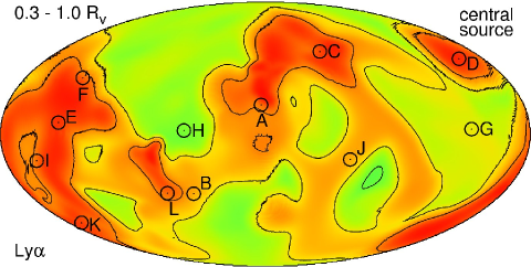
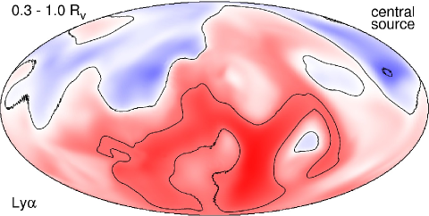
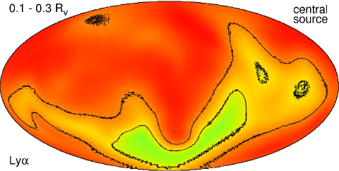
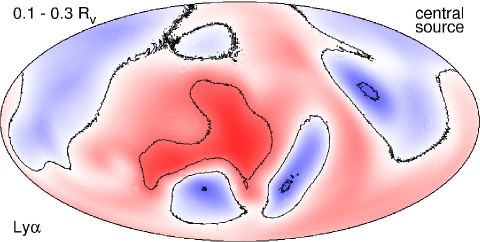
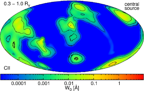
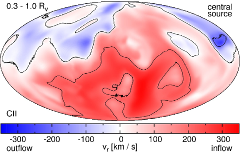
An EW can now be calculated for every angular position on the sky. With these numbers we can plot a whole full sky map of EW. This is done in the left panels of figure 8. There we show the resulting Hammer projections of EW for our fiducial galaxy. The upper two panels show ${\rm Ly}\alpha$ whereas the lowermost panel shows C ii. In the uppermost and lowermost panels the EWs were computed for the gas in the radius range between 0.3 and 1.0 $R_{\rm v}$ , whereas in the middle panels the EWs were determined for gas in a somewhat narrower and innermore radius range between 0.1 and 0.3 $R_{\rm v}$ . In the upper left panel the positions of the example line profiles from figure 6 are indicated by the circles with the letters attached to them. In the panels spanning the outer radius range one can again clearly see the narrow major streams having EWs of $>1$ Å ( ${\rm Ly}\alpha$ ) or $>0.01$ Å (C ii). One can also see the vast majority of the “stream-free” sky (as seen from the central galaxy) with EWs of $\sim 0.01$ Å ( ${\rm Ly}\alpha$ ) or $<10^{-5}$ Å (C ii). In the middle panel representing a narrow radius range very close to the central galaxy $(0.3R_{\rm v}>r>0.1R_{\rm v})$ this bi-modality is by far not as obvious as in the other two cases. This is due to the fact that at this distance from the galaxy centre the inflowing streams slowly dissipate into a region with more complex gas motions (“messy region”). Since the EWs are significantly lower for the C ii line and even lower for the other lines, as we will see later, we do not show Hammer projections of EW of other metal lines than C ii. We do show Hammer projections of EW-weighted velocity in the right panels of this figure. Positive velocities are inflowing into the galaxy (shown in red) and negative velocities are out of the galaxy (shown in blue). The contour lines indicate velocities of +200, 0 and -200 km s^-1. Regions with very high velocity outflows have a low EW, while velocities close to systemic velocity are at very high EW. This agrees very well with the high EW seen by S10 at $v_{\rm r}=0\,$ km s^-1. The velocity pattern of ${\rm Ly}\alpha$ and C ii is the same even if their EWs are so different. Comparing the upper two panels one can see that the distribution of velocities in the two different radius regimes varies. The term “outflow” can be misleading here. In our simulations some of the material that is receding from the centre of the galaxy is not necessarily diffuse gas driven by some kind of feedback processes. It could also be a clump or satellite galaxy which is merging with the central galaxy. It just had its first flyby with the central object and is therefore now “outflowing”.

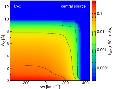
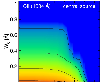
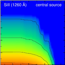
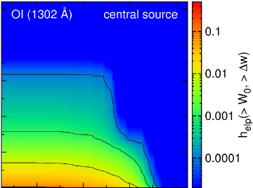
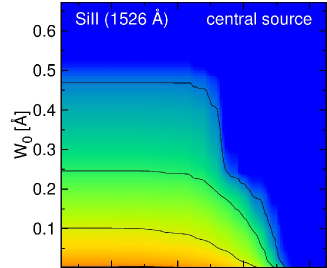
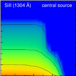
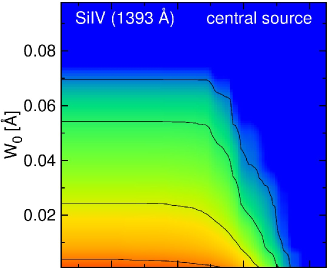
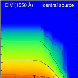
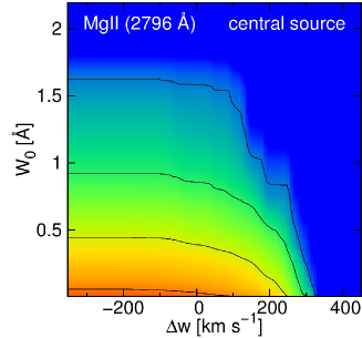
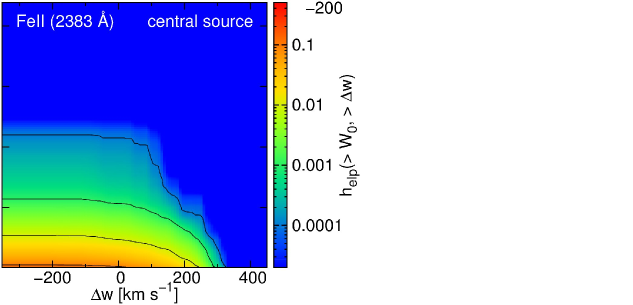
To present the statistics from these maps we determine the sky covering fractions. In figures 9 and 10 we show the fraction $f_{\rm c}$ of the sky as seen from the central galaxy that is covered with absorption line profiles which have EW higher than $W_{0}$ . Here we integrate in the central source geometry from 0.3 to 1.0 $R_{\rm v}$ . In figure 9 this is done for ${\rm Ly}\alpha$ whereas in figure 10 this is done for the metal lines (note the different x-axis scaling in both figures). We use our three simulated galaxies (resolution $70\,{\rm pc}$ ) at $z=2.3$ with $M_{\rm v}=3.5\times 10^{11}M_{\odot}$ and $R_{\rm v}=74\,$ kpc. These are shown in solid red in figure 9 and on the upper panels of figure 10. Again for better comparability with future observations we also use a second set of data consisting of two galaxies at $z=1.38$ with $M_{\rm v}=1.4\times 10^{12}M_{\odot}$ and $R_{\rm v}=150\,$ kpc. These are shown in dashed blue in figure 9 and on the upper panels of figure 10. We concentrate on the lines studied in great detail in S10 which are: ${\rm Ly}\alpha$ (1216 Å), C ii (1334 Å), O i (1302 Å), Si ii (1260 Å, 1304 Å and 1526 Å), C iv (1548 Å and 1550 Å) as well as Si iv (1393 Å and 1402 Å). In addition to these ten lines observed by S10 we also use here seven new ones: Mg ii (2803 Å and 2796 Å) and Fe ii (2600 Å, 2383 Å, 2344 Å, 2587 Å and 2374 Å). These lines have not been observed in this geometry or redshift range yet, but may be very suitable for future observational programmes at $z\sim 1$ . For ${\rm Ly}\alpha$ one can see that at higher redshift there is a higher covering fraction of large EW, implying that the streams are much more pronounced. The C iv and Si iv lines in the middle panels of figure 10 clearly stand out since they reach covering fractions as high as unity but for low column densities only. This is because these lines can be produced in the hot and diffuse medium whereas all the others can only be produced in cold gas only. Another interesting feature for the metal lines is that low ionised metal lines have higher peak values of EW by up to one order of magnitude, but low overall covering fraction. This is because low-ionised ions are more abundant in high-density, cold regions with low covering fraction, like streams.

As already mentioned earlier we want to show statistics of how many absorption lines show signatures of inflow versus how many absorption lines show signatures of outflow and how strong are those. This is done in figures 11 and 12. These figures are intended to give the likelihood of a detection of a cold stream while looking at a single galaxy from a single direction without averaging. They show the fraction $h_{\rm elp}$ of all possible example line profiles in the central geometry whose EW is higher than $W_{0}$ and whose line centre is at a velocity offset indicating an inflow at least as fast as $\Delta w$ . The example line profiles are integrated from $1.0\,R_{\rm v}$ down to $0.3\,R_{\rm v}$ . Positive velocities are inflowing into the galaxy and negative velocities are out of the galaxy. In these two figures no velocity degrading is used. The ${\rm Ly}\alpha$ panel shows that the probability of detecting an inflow which is flowing in with at least 150 km s^-1 with a signal of at least 3.9 Å in a single observation of a single galaxy without averaging is $\sim 4\,\%$ . In C ii one sees an inflow $>150$ km s^-1 with an EW $>$ 0.17 Å in 0.4 % of all observations. For Mg ii one sees an inflow $>150$ km s^-1 with an EW $>$ 0.2 Å in 1.3 % of all observations. These values should be achievable by future observations. Since it is the likely scenario that the inflowing streams and the wide-angle outflowing gas avoid each other to a great extent the streams as measured in our simulations where the outflows are a factor of 2-3 weaker than in the extreme observed cases can be regarded as a sensible approximation.

As a last application for this geometry we mimic the S10 stacking procedure (see their figures 6 and 10) they used to increase the signal to noise ratio. They stacked 89 galaxies with $z=2.3\pm 0.3$ to investigate the kinematics of the galaxy-scale outflows. We produce stacked spectra using our simulations by summing up the line profiles of several thousand different directions for each of the three galaxies and stack them together. We determine the absorption line profile for a spherical shell between an outer radius and an inner radius $r_{\rm i}$ . The outer radius is always kept constant at 1.0 $R_{\rm v}$ which corresponds roughly to 74 kpc. The inner radius $r_{\rm i}$ however is varied between 0.3 $R_{\rm v}$ and 0.02 $R_{\rm v}$ . This is done for the following reason: As one can see from figure 1, there are very clean, unperturbed streams into the galaxy down to as far as $\sim 0.25R_{\rm v}$ . In the immediate vicinity of the galaxy there is the “messy region” without well defined streams and with no well defined gas disk either. The galactic disk itself has no sharp edge and therefore its extent is not determined easily either. In order to account for these uncertainties we show several different absorption line profiles for different inner radii for every wavelength in question. All are averaged in the aforementioned way. In figures 13 and 14 the resulting profiles are shown for all the lines. These figures can be directly compared to figures 6 or 10 in S10. The plots reveal that we have for ${\rm Ly}\alpha$ a FWHM $\eta$ of up to $\sim 1900$ km s^-1 with a line depth of up to 0.90 for an inner radius $r_{\rm i}$ going as deep as 0.02 $R_{\rm v}$ (1.5 kpc). The ${\rm Ly}\alpha$ lines for high $r_{\rm i}$ having a shallow total MLD show very extended wings at the edges of the line profile whereas lines for small $r_{\rm i}$ having a deep total MLD the edges of the profiles are much sharper since the centre of the line is much deeper. All profiles of all lines always peak in the positive, indicating inflow. Our strongest metal line is Si ii. It has a maximum line depth of $\sim 0.23$ with a $\eta\sim 250\,$ km s^-1 for $r_{\rm i}=0.02\,R_{\rm v}$ . This confirms our initial guess that metal lines are so much weaker than the ${\rm Ly}\alpha$ line, since the inflowing material is mainly unprocessed primordial gas with very low metallicity. The predicted metal line absorption profiles appear tiny compared to the corresponding lines presented in figures 6 or 10 of S10 having a line depth of 0.5 and $\eta\sim 1000$ km s^-1 in metals. Detailed comparisons between our values and the observed values by S10 are given in Table 2.

ion	$\lambda_{0}$	MLD	$W_{0}$	MLD	$\eta$	$W_{0}$
		S10’s	S10’s	our	our	our
	[Å]		[Å]		[km s^-1]	[Å]
${\rm Ly}\alpha$	1216			0.90	1900	6.2
C ii	1334	0.5	1.6	0.16	250	0.20
Si ii	1260			0.23	250	0.25
O i	1302	0.7	2.7	0.15	250	0.16
Si ii	1526	0.6	1.8	0.11	200	0.13
Si ii	1304	0.7	2.4	0.12	200	0.12
C iv	1548	0.5	3.1	0.013	350	0.024
Si iv	1393	0.4	1.3	0.021	300	0.032
C iv	1550	0.5	3.4	0.015	350	0.027
Si iv	1402	0.3	0.8	0.019	300	0.027
Mg ii	2796			0.20	250	0.47
Fe ii	2383			0.14	250	0.27

Table 2: Comparison of maximum line depths (MLD), FWHM

\eta

and EW

W_{0}

in the central geometry between S10’s observations (their figure 10) and our predictions from the simulations (the “

r_{\rm i}=0.02\ R_{\rm v}

” line in our figures 13 and 14).

It is hard to compare our ${\rm Ly}\alpha$ absorption line profiles to the observations of S10 as they actually show emission line profiles. One could still draw interesting conclusions by comparing the underlying optical depths $\tau$ of the S10 observations with our simulations. However, the ${\rm Ly}\alpha$ emission is not only an indicator of cold streams. Probably the most suitable lines for the purpose of detecting cold streams in absorption are C ii and Mg ii since they have the strongest signal. Out of those Mg ii is closer to being observed with the needed sensitivity and resolution (cf. for example Matejek & Simcoe, 2012). As S10 point out, the easiest way for a ${\rm Ly}\alpha$ photon to reach the observer is to acquire the velocity of the outflowing material on the far side of the galaxy, and to be emitted in the observer’s direction. In this case the photon is redshifted by several hundred km s^-1 relative to the bulk of the material through which it must pass to reach us. This picture would explain qualitatively why the dominant component of ${\rm Ly}\alpha$ emission always appears redshifted relative to the galaxy systemic velocity (see e.g, Pettini et al., 2002; Adelberger et al., 2003), implying that their results for ${\rm Ly}\alpha$ have to be interpreted with caution. Our results for ${\rm Ly}\alpha$ absorption in the simulations are not subject to this complication, therefore one should be cautious when comparing our ${\rm Ly}\alpha$ results to the S10 data. Metal lines are less problematic.

\psfrag{relative intensity}[B][B][1][0]{relative intensity}\psfrag{vks}[B][B][1][0]{$\Delta w$ [km s${}^{-1}$]}\psfrag{lya}[Br][Br][1][0]{${\rm Ly}\alpha$}\psfrag{cg}[Br][Br][1][0]{central source}\psfrag{r30}[Br][Br][1][0]{{\color[rgb]{1,0,0}$r_{\rm i}=0.30\ R_{\rm v}$}}\psfrag{r20}[Br][Br][1][0]{{\color[rgb]{0,1,0}$r_{\rm i}=0.20\ R_{\rm v}$}}\psfrag{r10}[Br][Br][1][0]{{\color[rgb]{0,0,1}$r_{\rm i}=0.10\ R_{\rm v}$}}\psfrag{r05}[Br][Br][1][0]{{\color[rgb]{1,0,1}$r_{\rm i}=0.05\ R_{\rm v}$}}\psfrag{r02}[Br][Br][1][0]{{\color[rgb]{0,1,1}$r_{\rm i}=0.02\ R_{\rm v}$}}\includegraphics[width=240.42569pt]{XXline14Dvoigtvsrz01.eps}

Figure 13:

{\rm Ly}\alpha

absorption line profile for a central source geometry averaged over different viewing angles and all three galaxies. We integrated from 1.0

R_{\rm v}

down to different inner radii

r_{\rm i}

. Positive velocities are inflowing into the galaxy and negative velocities are out of the galaxy. Note the different scaling of both axes in comparison to figure 14. The profiles always peak in the positive, indicating inflow. Lines for high

r_{\rm i}

having a shallow total MLD show very extended wings at the edges of the distribution whereas lines for small

r_{\rm i}

having a deep total MLD the edges of the profiles are much sharper since the centre of the line is much deeper.

\psfrag{relative intensity}[B][B][1][0]{relative intensity}\psfrag{vks}[B][B][1][0]{$\Delta w$ [km s${}^{-1}$]}\psfrag{cg}[Bl][Bl][1][0]{central source}\psfrag{r30}[Br][Br][1][0]{{\color[rgb]{1,0,0}$r_{\rm i}=0.30\ R_{\rm v}$}}\psfrag{r20}[Br][Br][1][0]{{\color[rgb]{0,1,0}$r_{\rm i}=0.20\ R_{\rm v}$}}\psfrag{r10}[Br][Br][1][0]{{\color[rgb]{0,0,1}$r_{\rm i}=0.10\ R_{\rm v}$}}\psfrag{r05}[Br][Br][1][0]{{\color[rgb]{1,0,1}$r_{\rm i}=0.05\ R_{\rm v}$}}\psfrag{r02}[Br][Br][1][0]{{\color[rgb]{0,1,1}$r_{\rm i}=0.02\ R_{\rm v}$}}\psfrag{CII}[Bl][Bl][1][0]{{C\,{ii}} (1334 \AA)}\psfrag{OI}[Bl][Bl][1][0]{{O\,{i}} (1302 \AA)}\psfrag{SiIIa}[Bl][Bl][1][0]{{Si\,{ii}} (1526 \AA)}\psfrag{SiIIb}[Bl][Bl][1][0]{{Si\,{ii}} (1260 \AA)}\psfrag{CIVa}[Bl][Bl][1][0]{{C\,{iv}} (1548 \AA)}\psfrag{SiIVa}[Bl][Bl][1][0]{{Si\,{iv}} (1393 \AA)}\psfrag{CIVb}[Bl][Bl][1][0]{{C\,{iv}} (1550 \AA)}\psfrag{SiIVb}[Bl][Bl][1][0]{{Si\,{iv}} (1402 \AA)}\psfrag{SiIIc}[Bl][Bl][1][0]{{Si\,{ii}} (1304 \AA)}\psfrag{MgIIb}[Bl][Bl][1][0]{{Mg\,{ii}} (2796 \AA)}\psfrag{FeIIb}[Bl][Bl][1][0]{{Fe\,{ii}} (2383 \AA)}\includegraphics[width=168.44026pt]{XXline14Dvoigtvsrz02.eps}

Figure 14: Same absorption line profiles for a central source as in figure 13, this time for the metal lines. Positive velocities are inflowing into the galaxy and negative velocities are out of the galaxy. Note the different y-axis scaling from row to row and the different overall axes scaling with respect to figure 13. The metal lines are much weaker than the

{\rm Ly}\alpha

line, since the inflowing material is mainly unprocessed primordial gas with very low metallicity. These metal lines also appear tiny compared to the corresponding lines presented by S10. The profiles always peak in the positive, indicating inflow. The lines with the strongest signals are Si ii and Mg ii. A more detailed quantitative comparison to the observations is presented in table 2.

There are two main conclusions from our analysis of the central-source geometry, which are discouraging concerning the potential for detecting cold streams. First stacking of absorption line profiles does not strengthen but weakens the signature of cold streams this might be counter intuitive, but compare figure 6 with figures 13 and 14). See figures 11 and 12 for the predicted strengths of a cold stream absorption signal when observing without stacking. Second, the ${\rm Ly}\alpha$ signal detected by observations is naturally dominated by outflows which are expected to have much higher covering factor and metallicity (Faucher-Giguere & Keres, 2011).

\psfrag{bRv}[B][B][1][0]{$b$ $[R_{\rm v}]$}\psfrag{Ncm2}[B][B][1][0]{$N_{\rm Ai}$ [cm${}^{-2}$]}\psfrag{HI}[B][B][1][0]{{\color[rgb]{1,0,0}H\,{i}}}\psfrag{CII}[B][B][1][0]{{\color[rgb]{0,1,0}C\,{ii}}}\psfrag{CIV}[B][B][1][0]{{\color[rgb]{0,0,1}C\,{iv}}}\psfrag{OI}[B][B][1][0]{{\color[rgb]{1,0,1}O\,{i}}}\psfrag{SiII}[B][B][1][0]{{\color[rgb]{0,1,1}Si\,{ii}}}\psfrag{SiIV}[B][B][1][0]{{\color[rgb]{0,0,0}Si\,{iv}}}\psfrag{bg}[Bl][Bl][1][0]{background source}\includegraphics[width=240.42569pt]{XXcovfrac23den.eps}

Figure 16: Area weighted average column density

N_{\rm Ai}

as a function of impact parameter

b

for H i and five different metal lines in the background source geometry. The H i column density decreases through the interaction region in the greater disc vicinity, from 10²² cm⁻² near the centre of the galaxy to 10²⁰ cm⁻² at 0.5

R_{\rm v}

. It remains roughly constant at 10¹⁹ cm⁻² in the stream regime out to 1.5

R_{\rm v}

, and is not much lower out to 2.5

R_{\rm v}

5 Background source

In this section we consider the ${\rm Ly}\alpha$ and metal line absorption that occurs as UV light emitted by a background galaxy or a quasar is absorbed by gas in the circum-galactic environment of the foreground galaxy under investigation. In this geometry one cannot distinguish between inflowing and outflowing gas. However, the distribution of impact parameters allows us to explore the spatial distribution of the circum-galactic gas surrounding the foreground galaxies. S10 constructed a sample of 512 close angular pairs, $(1-15^{\prime\prime})$ , of galaxies in the redshift range $z\sim 2-3$ with a large redshift difference such that one is at the background of the other with no physical association. The pair separations correspond to galactocentric impact parameters in the range $3-125$ kpc (physical) at $z=2.2$ , providing a map of cool gas as a function of galactocentric distance for a well-characterised population of galaxies. The discussion in this section will lead to a prediction of absorption line profiles that are directly comparable to the ones observed and published in section 6 of S10.

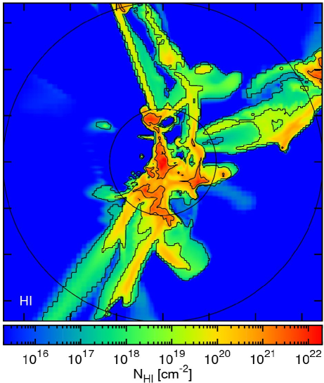
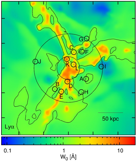
For a first impression of the simulation data in the background-source geometry we show in figure 15 a map of projected neutral hydrogen column density. The box of $140\,{\rm kpc}$ is centred on our fiducial galaxy of $M_{\rm v}\simeq 4\times 10^{11}M_{\odot}$ at $z=2.3$ , which serves as the foreground galaxy. The column density $N_{\rm Ai}(x,y)$ of element $A$ and ionisation state $i$ at the position $(x,y)$ itself is now calculated by

N_{\rm Ai}(x,y)=\int^{\rm bs}_{\rm-bs}x_{\rm Ai}(\vec{x})\ n_{\rm A}(\vec{x})\ dz,

(7)

where $bs$ indicates the box size of twice the virial radius, $n_{\rm A}(\vec{x})$ is the total gas density of element $A$ at position $\vec{x}=(x,y,z)$ and $x_{\rm Ai}$ is the ionisation fraction of element $A$ in state $i$ . This equation is the analog of equation 1 for the central geometry. The map in figure 15 corresponds to figure 3 in the central geometry. The outer circle marks the virial radius and the inner circle is at $1/3\ R_{\rm v}$ . Contours are shown for $10^{17}$ , $10^{19}$ and $10^{21}\,{\rm cm}^{-2}$ . One can see the three major streams which are very pronounced outside $1/3\ R_{\rm v}$ . They have neutral hydrogen column densities of $N_{\rm HI}>10^{17}$ cm^-2. The background outside $1/3\ R_{\rm v}$ has neutral hydrogen column densities of $N_{\rm HI}<10^{15}$ cm^-2. In the messy region inside $1/3\ R_{\rm v}$ one cannot distinguish between streams, galactic disk or background. The neutral hydrogen column densities within this region vary between $10^{15}$ cm^-2 and $10^{17}$ cm^-2. One should note that this ideal map cannot be directly compared to any observed galaxy, because it requires a background point source along the same line of sight of each pixel in the map.

The impression from figure 15 is that the column density tends to decrease with increasing distance from the galaxy centre. Figure 16 shows the area-weighted average column density, for H i and five different metal lines, as a function of the impact parameter $b$ . The H i column density decreases through the interaction region in the greater disc vicinity, from 10²² cm^-2 near the centre of the galaxy to 10²⁰ cm^-2 at 0.5 $R_{\rm v}$ . It remains roughly constant at 10¹⁹ cm^-2 in the stream regime out to 1.5 $R_{\rm v}$ , and is not much lower out to 2.5 $R_{\rm v}$ . The metal ionisation states also decrease inside 0.5 $R_{\rm v}$ and are roughly constant at values between 10¹⁴ cm^-2 (O i) and 10¹¹ cm^-2 (Si iv) in the outer halo and beyond.

\psfrag{relative intensity}[B][B][1][0]{relative intensity}\psfrag{bg}[Bl][Bl][1][0]{background source}\psfrag{corrfig}[Bl][Bl][1][0]{see figure \ref{fig:EWgalmap}}\psfrag{vks}[B][B][1][0]{$\Delta w$ [km s${}^{-1}$]}\psfrag{lya}[Bl][Bl][1][0]{${\rm Ly}\alpha$}\psfrag{A}[B][B][1][0]{A}\psfrag{B}[B][B][1][0]{B}\psfrag{C}[B][B][1][0]{C}\psfrag{D}[B][B][1][0]{D}\psfrag{E}[B][B][1][0]{E}\psfrag{F}[B][B][1][0]{F}\psfrag{G}[B][B][1][0]{G}\psfrag{H}[B][B][1][0]{H}\psfrag{I}[B][B][1][0]{I}\psfrag{J}[B][B][1][0]{J}\psfrag{K}[B][B][1][0]{K}\psfrag{L}[B][B][1][0]{L}\psfrag{NHI=2.9e15}[Bl][Bl][1][0]{$N_{\rm HI}=3.8\times 10^{15}$ cm${}^{-2}$}\psfrag{NHI=4.3e19}[Bl][Bl][1][0]{$N_{\rm HI}=2.6\times 10^{19}$ cm${}^{-2}$}\psfrag{NHI=4.6e20}[Bl][Bl][1][0]{$N_{\rm HI}=3.2\times 10^{20}$ cm${}^{-2}$}\psfrag{NHI=3.0e19}[Bl][Bl][1][0]{$N_{\rm HI}=9.3\times 10^{19}$ cm${}^{-2}$}\psfrag{NHI=6.8e13}[Bl][Bl][1][0]{$N_{\rm HI}=6.8\times 10^{13}$ cm${}^{-2}$}\psfrag{NHI=5.4e13}[Bl][Bl][1][0]{$N_{\rm HI}=6.1\times 10^{13}$ cm${}^{-2}$}\psfrag{NHI=1.3e13}[Bl][Bl][1][0]{$N_{\rm HI}=1.3\times 10^{13}$ cm${}^{-2}$}\psfrag{NHI=3.3e14}[Bl][Bl][1][0]{$N_{\rm HI}=3.0\times 10^{14}$ cm${}^{-2}$}\psfrag{NHI=4.1e21}[Bl][Bl][1][0]{$N_{\rm HI}=2.3\times 10^{21}$ cm${}^{-2}$}\psfrag{NHI=7.3e19}[Bl][Bl][1][0]{$N_{\rm HI}=1.2\times 10^{20}$ cm${}^{-2}$}\psfrag{NHI=}[Bl][Bl][1][0]{$N_{\rm HI}=$}\psfrag{1.4e18}[Bl][Bl][1][0]{$1.2\times 10^{18}$ cm${}^{-2}$}\psfrag{3.8e18}[Bl][Bl][1][0]{$2.6\times 10^{18}$ cm${}^{-2}$}\psfrag{W0=0.68A}[Bl][Bl][1][0]{$W_{0}=0.68$ \AA}\psfrag{W0=1.2A}[Bl][Bl][1][0]{$W_{0}=1.2$ \AA}\psfrag{W0=2.6A}[Bl][Bl][1][0]{$W_{0}=2.6$ \AA}\psfrag{W0=6.1A}[Bl][Bl][1][0]{$W_{0}=6.1$ \AA}\psfrag{W0=3.7A}[Bl][Bl][1][0]{$W_{0}=3.7$ \AA}\psfrag{W0=1.0A}[Bl][Bl][1][0]{$W_{0}=1.0$ \AA}\psfrag{W0=0.19A}[Bl][Bl][1][0]{$W_{0}=0.19$ \AA}\psfrag{W0=0.17A}[Bl][Bl][1][0]{$W_{0}=0.17$ \AA}\psfrag{W0=0.043A}[Bl][Bl][1][0]{$W_{0}=0.043$ \AA}\psfrag{W0=0.50A}[Bl][Bl][1][0]{$W_{0}=0.50$ \AA}\psfrag{W0=7.6A}[Bl][Bl][1][0]{$W_{0}=7.6$ \AA}\psfrag{W0=3.3A}[Bl][Bl][1][0]{$W_{0}=3.3$ \AA}\includegraphics[width=155.6366pt]{XXline15Dvoigtz01.eps}

Figure 18: Example

{\rm Ly}\alpha

absorption line profiles seen from a single direction in the background geometry integrated from 0.3 to 1.0

R_{\rm v}

. For a background source one cannot tell from the redshift or blueshift of the line relative to the central restframe whether it represents inflow or outflow with respect to the galaxy centre. From inspection of the three-dimensional information in the simulations, we know that almost in every case a significant coherent shift of the line is associated with inflow. Values for neutral hydrogen column density and EW are quoted in each panel. Uppermost panel: various modes of bimodal streaming, intermediate upper panel: different examples of strong unidirectional streaming, intermediate lower panel: low absorption profiles and lowermost panel: extraordinary cases. Some of the lines are saturated like B, C, D, E, F, K and L, whereas others are not. The letters correspond to the indicated position of the map from figure 20.

Figure 19: Same figure as figure 18, panel K (the panel with the deepest signal) this time for selected metal lines providing also the deepest signal, namely: C ii (1334 Å), Si ii (1260 Å), Mg ii (2796 Å) and Fe ii (2383 Å). Panel K is fully saturated in

{\rm Ly}\alpha

but still shows peak absorption line depths of 0.25 and EW of

\sim 0.2

Å for these metal lines. The C ii panel of this plot shows slight differences with the results of Kimm et al. (2011, their figure 2, lower panel) due to different line computing algorithms.

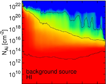
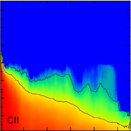
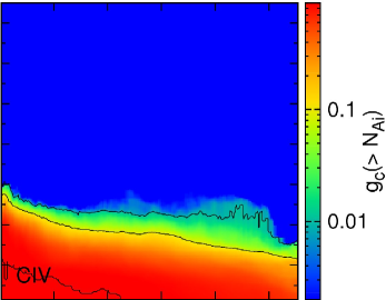
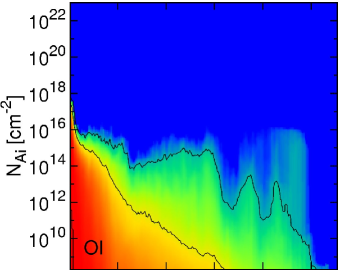
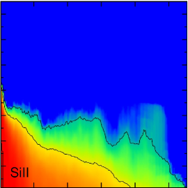
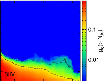
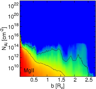
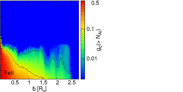
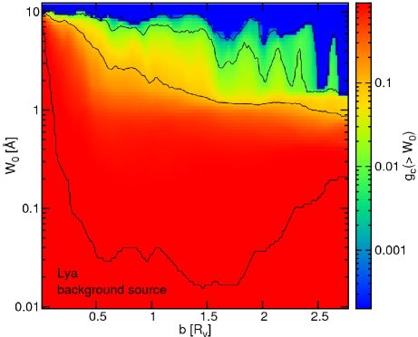
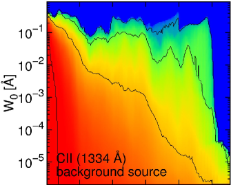
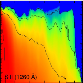
Figure 15 is limited to the angle-averaged column density. Figure 17 presents the distribution of column densities, for the purpose of evaluating the likelihood of an observation through a given line of sight. We plot area covering fractions $g_{\rm c}$ as a function of impact parameter $b$ and cumulative column density $N_{\rm Ai}$ . The values are averaged over three different galaxies and three orthogonal projections per galaxy. The panels show for every impact parameter $b$ the fraction of the area within an annulus of radius $b$ and width $\delta b$ which has a column density of $N_{\rm Ai}$ or above. One can see that there are obviously much higher columns of H i present than of the other metal ionisation state. H i has column densities which are several orders of magnitude higher, depending on the actual radius and the area covering fraction one wants to look at. The columns of the metal ionisation states lie closely to each other and decrease rather smoothly with increasing radius. The $g_{\rm c}=0.1$ lines of the two carbon lines are fairly similar, both fall off almost linearly from $\sim 10^{15}$ cm^-2 at the left edge of the graph to $\sim 10^{10}$ cm^-2 at the right edge of the graph. This is also true for the $g_{\rm c}=0.1$ lines of the two silicon lines. They fall off from around $10^{14}$ to below $10^{8}$ . The $g_{\rm c}=0.01$ line, which lies much higher, on the other hand has more differences between the low-ionised metals (like C ii, Si ii or Fe ii) on the higher ionised metals (like C iv or Si iv): In case of the low-ionised metals the line has considerably more features like the extended bumps at impact parameters of $1.0\ R_{\rm v}$ or $2.0\ R_{\rm v}$ . The distribution for C ii indicates the highest, the one for Mg ii indicates the lowest overall column densities.

The H i panel of figure 17 is comparable to figure 4 of F11, who implemented a full radiative transfer calculation. A comparison between the two allows us to evaluate the accuracy of our simplified treatment of self-shielding. For impact parameter other than $b=2.0\ R_{\rm v}$ the latter show in their figure 4 values which are normalised to the value it would have at $b=2.0\ R_{\rm v}$ . In the following we will only quote the un-normalised values. In our results the same covering factors correspond to column densities that are usually smaller by a factor of $\sim 3$ . For example at $b=2.0\ R_{\rm v}$ F11 have a covering factor of 0.01 at $3\times 10^{20}$ cm^-2 and of 0.1 at $10^{17}$ cm^-2. In our results these covering factors correspond to column densities of $10^{20}$ cm^-2 and $3\times 10^{16}$ cm^-2, respectively. The H i panel of figure 17 is also roughly comparable to Table 1 of Faucher-Giguere & Keres (2011). In our results we have covering factors which are on average smaller by a factor of 1.5. For example at $b=0.5\ R_{\rm v}$ they have an average covering factor of $\sim 0.3$ at $10^{17.2}\lower 2.15277pt\hbox{$\;\buildrel<\over{\sim}\;$}N_{\rm HI}\lower 2.15277pt\hbox{$\;\buildrel<\over{\sim}\;$}2\times 10^{20}$ and of $\sim 0.08$ at $>2\times 10^{20}$ cm^-2. Our corresponding covering factors are 0.2 and 0.1. In their figure 10, Shen et al. (2012) quote a H i covering factor of column densities higher than $10^{17.2}$ cm^-2 for $r<R_{\rm v}$ ( $r<2R_{\rm v}$ ) of 27% (10%). Our corresponding covering factors are 0.2 and 0.5. We conclude that our results based on the simplified treatment of self-shielding (section 3) provide a rather good approximation to the results from the full radiative transport analysis.

\psfrag{EW}[B][B][1][0]{$W_{0}$ [\AA]}\psfrag{rRv}[B][B][1][0]{$b$ $[R_{\rm v}]$}\psfrag{bg}[Bl][Bl][1][0]{background source}\psfrag{La}[Bl][Bl][1][0]{${\rm Ly}\alpha$}\psfrag{CDB sim}[Br][Br][1][0]{{\color[rgb]{1,0,0}{CDB} simulation}}\psfrag{S10 obs}[Br][Br][1][0]{{\color[rgb]{0,0,1}{S10} observation}}\psfrag{CII}[Br][Br][1][0]{{\color[rgb]{1,0,0}{C\,{ii}} (1334 \AA)}}\psfrag{CIVa}[Br][Br][1][0]{{\color[rgb]{0,1,1}{C\,{iv}} (1548 \AA)}}\psfrag{OI}[Br][Br][1][0]{{\color[rgb]{0,1,0}{O\,{i}} (1302 \AA)}}\psfrag{SiIIa}[Br][Br][1][0]{{\color[rgb]{0,0,1}{Si\,{ii}} (1526 \AA)}}\psfrag{SiIVa}[Br][Br][1][0]{{\color[rgb]{0,0,0}{Si\,{iv}} (1393 \AA)}}\psfrag{CIVb}[Br][Br][1][0]{{\color[rgb]{1,0,0}{C\,{iv}} (1550 \AA)}}\psfrag{SiIIb}[Br][Br][1][0]{{\color[rgb]{1,0,1}{Si\,{ii}} (1260 \AA)}}\psfrag{SiIVb}[Br][Br][1][0]{{\color[rgb]{0,1,0}{Si\,{iv}} (1402 \AA)}}\psfrag{SiIIc}[Br][Br][1][0]{{\color[rgb]{0,1,1}{Si\,{ii}} (1304 \AA)}}\includegraphics[width=157.91287pt]{XXgalmap14Dvoigtz3.eps}

Figure 21: Average EW

W_{0}

as a function of impact parameter

b

, averaged over the three simulated galaxies. For

{\rm Ly}\alpha

, we show for comparison the observational results of S10 (their Table 4). The inner galaxy is responsible for a steep peak in EWs in the range

b\leq 0.5R_{\rm v}

. Outside of this radius the EW is lower and it shows an overall gradually declining with

b

. As expected there is a strong negative correlation between impact parameter

b

and EW. This behaviour is the same for all ten lines. The

{\rm Ly}\alpha

and the Si ii (1260 Å) lines agree with the theoretical results of F11 (their figure 14). The

{\rm Ly}\alpha

line also agrees with the theoretical results of Shen et al. (2012) (their figure 9). The observational results of S10 for

{\rm Ly}\alpha

(their Table 4 and their figure 21) are also in fairly good agreement.

We next compute example absorption line profiles for a background source, in analogy to the line profiles for a central source, using equations (2) to (5). From now on, we apply a Gaussian point spread function with a beamsize (= FWHM) of 4 kpc, following the algorithm described in section 4. In addition, the velocity resolution is now downgraded to 50 km s^-1, to match the velocity resolution used in the corresponding figures of S10. In figure 18 and 19 we show a selection of absorption line profiles, for ${\rm Ly}\alpha$ and metal lines, respectively, demonstrating a large variety. These figures are the analogs of figures 6 and 7 for a central source. Some line profiles show a single dominant stream, others indicate two streams, some display weak absorption and others show strong absorption. For a background source one cannot tell from the redshift or blueshift of the line relative to the central restframe whether it represents inflow or outflow with respect to the galaxy centre. From inspection of the three-dimensional information in the simulations, we know that almost in every case a significant coherent shift of the line is associated with inflow. In the case of ${\rm Ly}\alpha$ , 7 out of 12 lines in the sample are saturated (B, C, D, E, F, K, L). Panel K, which shows the strongest absorption in ${\rm Ly}\alpha$ , has for selected metal lines a maximum absorption depths of only 0.25 and an equivalent width EW of only $\sim 0.2$ Å. Some of the weaker ${\rm Ly}\alpha$ lines (e.g, panels I or even H) might be completely erased by noise and the ISM component at $v=0$ . The leftmost panel of figure 19 is analogous to the lower panel of figure 3 in Kimm et al. (2011). The latter obtain for C ii a maximum line depth of $\sim 0.9$ with a FWHM $\eta$ of 650 km s^-1. The difference from our result most likely stems from the fact that they used a simulation with a resolution lower by a factor of 20, the Horizon MareNostrum simulation (Ocvirk, Pichon & Teyssier, 2008), and addressed haloes more massive by a factor of a few. Furthermore, they used a different prescription for the Gaussian velocity distribution, where they obtained their velocity dispersion from the neighbouring 26 cells instead of the more appropriate algorithm described in equations (2) to (4).

As for the central source, we compute the equivalent widths from the absorption line profiles using equation (6). The EWs for a background source are mapped for our fiducial galaxy in figure 20. The outer circle marks the virial radius and the inner circle is at $1/3\,R_{\rm v}$ . This plot is the analog of figure 8 for a central source. The EWs shown in it span two and a half orders of magnitude. The three major streams are fairly prominent, in addition to the central region in the greater vicinity of the disc. Also very prominent are the parts of the IGM which are stream-less.

Figure 20 illustrates the dependence of the EWs on the projected distance from the centre, or impact parameter $b$ . In the galaxy vicinity at the halo centre, $b<10\,{\rm kpc}$ , say, we see the highest absorption, which gradually declines toward larger radii, as the volume becomes dominated by the dilute medium between the streams. Figure 21 shows the average EW as a function of impact parameter $b$ , averaged over the three simulated galaxies at $z=2.3$ , where the virial masses are $M_{\rm v}\simeq 4\times 10^{11}M_{\odot}$ . For ${\rm Ly}\alpha$ , we show for comparison the observational results of S10 (their Table 4), assuming a virial radius of 74 kpc. In our simulation results for all the lines, the inner galaxy is responsible for a steep peak in EWs in the range $b\leq 0.5R_{\rm v}$ . Outside of this radius the EW is lower and it shows an overall gradually declining with $b$ . A comparison with the observations shown in figure 21 of S10 indicates that the observational EW for the ${\rm Ly}\alpha$ line lies a factor of two or less below our predicted value at low $b$ , and is consistent with our prediction at larger radii. The simulation results in figure 14 of F11 and in figure 9 of Shen et al. (2012) for ${\rm Ly}\alpha$ are in excellent agreement with our current results, and so are the F11 predictions for Si ii (1260 Å). The observational results of S10 for the EW of the metal lines are two orders of magnitude above our predictions. These are likely to reflect massive, cold, dense and metal-rich outflows that are not reproduced in an appropriate amplitude in our simulations.

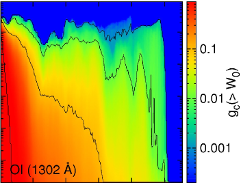
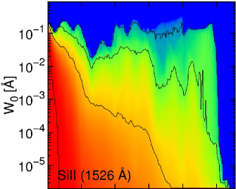
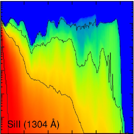
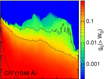
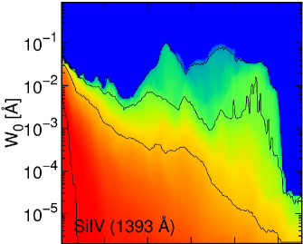
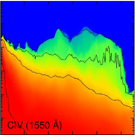
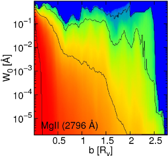
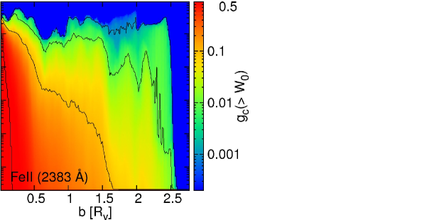
The probability to observe a given EW along a given line of sight of impact parameter $b$ is shown in figures 22 and 23. Shown in colour is the area covering fraction $g_{\rm c}$ as a function of impact parameter $b$ and cumulative EW for different absorption lines. The panels show for every impact parameter bin $b$ the fraction of the area within this impact parameter bin which has an EW of the indicated value $W_{0}$ or above. The contours mark fractions of 1.0, 0.1, 0.01 and 0.001. The values are averaged over three different galaxies and three orthogonal projections, in both directions each. This figure is the analog of figure 10 for a central source. We see that in ${\rm Ly}\alpha$ we have EWs $>0.01$ Å everywhere. Peak EWs go as high as 10 Å. The 0.1 area covering fraction line is falling monotonically with $b$ , whereas the 0.01 and 0.001 lines show noisy distortions at $b>1.5\ R_{\rm v}$ . For the metal lines the peak EWs lie near 0.1 Å and their minimum values are well below 10^-6 Å. In all cases the EWs are declining mainly monotonic with radius. For ${\rm Ly}\alpha$ the decline is rather gradual, only by an order of magnitude over the studied radius range. For the metal lines the decline is by more than five orders of magnitude. We see some noisy distortions in the high $b$ , low $g_{\rm c}$ regime. Over all the strongest lines are C ii and Mg ii.

Finally, we try to produce absorption line profiles that could be compared to those presented in figures 6 and 10 of S10. They stacked spectra of several galaxies in order to increase the signal to noise ratio. Their sample contains 512 close $(1^{\prime\prime}-15^{\prime\prime})$ angular pairs of $z\sim 2-3$ galaxies with redshift differences that indicate no physical association. The sample explores the cool gas as a function of galactocentric impact parameter in the range $3-125$ kpc (physical) at $z=2.2$ . In figures 24 and 25 we show the resulting absorption line profiles for ${\rm Ly}\alpha$ and metal lines in our simulations, stacked over six principal different viewing directions (three orthogonal axis in both directions). We show the line profiles for the same three different impact parameter bins as in S10: $10-41$ kpc, $41-82$ kpc and $82-125$ kpc. (Note the different scales in figures 24, 25 and from row to row within figure 25). The lines for $10-41$ kpc in those figures correspond to figure 18 in S10, the lines for $41-82$ kpc correspond to figure 19 in S10, and the lines for $82-125$ kpc correspond to figure 20 in S10. For ${\rm Ly}\alpha$ we have a FWHM $(=\eta)$ of up to $\sim 550$ km s^-1 and a relative intensity of 40-50% at the line centre of the innermost radius bin. It is not easy to compare our ${\rm Ly}\alpha$ absorption line profiles to the observations of S10 as they actually show emission line profiles. One could still draw interesting conclusions by comparing the underlying optical depths $\tau$ of the S10 observations with our simulations. However, due to the special transfer behaviour of ${\rm Ly}\alpha$ mentioned at the end of section 4 the ${\rm Ly}\alpha$ emission is not only an indicator of cold streams. Therefore the results have to be taken with caution. Our strongest metal absorption lines, Si ii and C ii, have both a maximum line depth of $\sim 0.015$ with $\eta\sim 350$ km s^-1 for the $10-41$ kpc bin. This appears tiny compared to the corresponding lines presented in figures 18 or 19 of S10 having a line depth of 0.2 and $\eta\sim 1000$ km s^-1. Detailed comparisons between our values and the observed values by S10 are given in Table 3.

ion	$\lambda_{0}$	$W_{0}$	MLD	$\eta$	$W_{0}$
		S10’s	our	our	our
	[Å]	[Å]		[km s^-1]	[Å]
${\rm Ly}\alpha$	(1216)	4.7	0.61	550	2.3
C ii	(1334)	2.61	0.016	350	0.025
Si ii	(1260)	2.01	0.012	400	0.019
O i	(1302)		0.0080	400	0.013
Si ii	(1526)	1.96	0.0038	400	0.0072
Si ii	(1304)		0.0030	400	0.0047
C iv	(1548)	3.90	0.0013	350	0.0023
Si iv	(1393)	2.04	0.00081	350	0.0013
C iv	(1550)	3.90	0.00068	350	0.0012
Si iv	(1402)		0.00041	350	0.00064
Mg ii	(2796)		0.0094	400	0.033
Fe ii	(2383)		0.0062	400	0.019

Table 3: Comparison of maximum line depths (MLD), FWHM

\eta

and EW

W_{0}

in the background geometry between S10’s observations (their Table 4, second line) and our predictions from the simulations (the “

10-41

kpc” line in our figures 24 and 25).

Figure 24 as well as the upper middle panel of figure 25 can be compared to figure 13 of F11. For ${\rm Ly}\alpha$ , in the $10-41$ kpc bin, the maximum line depth is 0.61 and 0.55 respectively, and the FWHM $\eta$ is 550 and 400 km s^-1 respectively. For Si ii (1260 Å), in the same $10-41$ kpc bin, the maximum depth is 0.013 and 0.05 respectively, and $\eta\sim 350$ km s^-1 in both. These results are similar. The upper left panel of figure 25 can be compared to the right panel of figure 3 in Kimm et al. (2011), where for C ii the maximum line depth is $\sim 0.65$ with a FWHM $\eta$ of 550 km s^-1. We identified three possible reasons for these differences: First Kimm et al. (2011) used a simulation²²2the Horizon MareNostrum simulation (Ocvirk, Pichon & Teyssier, 2008) with a maximum resolution of 1 kpc having a much lower resolution than we do. Second, the haloes they analysed are in a very different (much higher) mass range ( $M_{\rm v}>10^{12}$ M_⊙) than the haloes we use. Third and most importantly they use a different prescription for the Gaussian velocity distribution as described earlier. We conclude that stacking of the absorption lines from a background source tends to wash out the cold filament absorption signal (compare figure 18 with figures 24 and 25). Unlike the case of a central source, in the case of a background source the absorption by inflowing gas is not well separated from the absorption by outflowing gas.

\psfrag{relative intensity}[B][B][1][0]{relative intensity}\psfrag{vks}[B][B][1][0]{$\Delta w$ [km s${}^{-1}$]}\psfrag{bg}[Bl][Bl][1][0]{background source}\psfrag{Lya}[Bl][Bl][1][0]{${\rm Ly}\alpha$}\psfrag{1st}[Br][Br][1][0]{{\color[rgb]{0,0,1}$10-41$ kpc}}\psfrag{2nd}[Br][Br][1][0]{{\color[rgb]{0,1,0}$41-82$ kpc}}\psfrag{3rd}[Br][Br][1][0]{{\color[rgb]{1,0,0}$82-125$ kpc}}\includegraphics[width=240.42569pt]{XXline28Dvsrz01.eps}

Figure 24: Absorption line profiles for the background geometry for

{\rm Ly}\alpha

. The data are averaged over three different impact parameter bins, three different galaxies and six different viewing directions in the background geometry. Note the different x- and y-scales in this figure in comparison to Figure 25. This figure agrees with the results of F11 (their figure 13). A qualitative comparison to the observation is presented in table 3.

6 Conclusions

Theory, including hydrodynamical cosmological simulations, tells us that massive galaxies at high redshifts were fed by cold gas streams, inflowing into dark-matter haloes at high rates along the filaments of the cosmic web (Keres et al., 2005; Dekel & Birnboim, 2006; Dekel et al., 2009; Danovich et al., 2012), but observing this process is not straightforward. Here we addressed the expected absorption signature from these cold streams. We “observed” simulated galaxies for ${\rm Ly}\alpha$ absorption as well as metal lines from low and medium ionisation ions. We focused on the absorption line profiles as observed by Steidel et al. (2010), using their set of ten different lines and mimicking their way of stacking data from several galaxies, for sources that are either in the background or at the centre of the absorbing halo itself. The simulations used are zoom-in cosmological simulations with a maximum resolution of 35-70 pc (Ceverino, Dekel & Bournaud, 2010). Self-shielding was accounted for by a simple density criterion.

\psfrag{relative intensity}[B][B][1][0]{relative intensity}\psfrag{vks}[B][B][1][0]{$\Delta w$ [km s${}^{-1}$]}\psfrag{bg}[Bl][Bl][1][0]{background source}\psfrag{CII}[Bl][Bl][1][0]{{C\,{ii}} (1334 \AA)}\psfrag{OI}[Bl][Bl][1][0]{{O\,{i}} (1302 \AA)}\psfrag{SiIIa}[Bl][Bl][1][0]{{Si\,{ii}} (1526 \AA)}\psfrag{SiIIb}[Bl][Bl][1][0]{{Si\,{ii}} (1260 \AA)}\psfrag{SiIIc}[Bl][Bl][1][0]{{Si\,{ii}} (1304 \AA)}\psfrag{CIVa}[Bl][Bl][1][0]{{C\,{iv}} (1548 \AA)}\psfrag{SiIVa}[Bl][Bl][1][0]{{Si\,{iv}} (1393 \AA)}\psfrag{CIVb}[Bl][Bl][1][0]{{C\,{iv}} (1550 \AA)}\psfrag{SiIVb}[Bl][Bl][1][0]{{Si\,{iv}} (1402 \AA)}\psfrag{MgIIb}[Bl][Bl][1][0]{{Mg\,{ii}} (2796 \AA)}\psfrag{FeIIb}[Bl][Bl][1][0]{{Fe\,{ii}} (2383 \AA)}\psfrag{1st}[Br][Br][1][0]{{\color[rgb]{0,0,1}$10-41$ kpc}}\psfrag{2nd}[Br][Br][1][0]{{\color[rgb]{0,1,0}$41-82$ kpc}}\psfrag{3rd}[Br][Br][1][0]{{\color[rgb]{1,0,0}$82-125$ kpc}}\includegraphics[width=174.98427pt]{XXline28Dvsrz02.eps}

\psfrag{relative intensity}[B][B][1][0]{relative intensity}\psfrag{vks}[B][B][1][0]{$\Delta w$ [km s${}^{-1}$]}\psfrag{bg}[Bl][Bl][1][0]{background source}\psfrag{CII}[Bl][Bl][1][0]{{C\,{ii}} (1334 \AA)}\psfrag{OI}[Bl][Bl][1][0]{{O\,{i}} (1302 \AA)}\psfrag{SiIIa}[Bl][Bl][1][0]{{Si\,{ii}} (1526 \AA)}\psfrag{SiIIb}[Bl][Bl][1][0]{{Si\,{ii}} (1260 \AA)}\psfrag{SiIIc}[Bl][Bl][1][0]{{Si\,{ii}} (1304 \AA)}\psfrag{CIVa}[Bl][Bl][1][0]{{C\,{iv}} (1548 \AA)}\psfrag{SiIVa}[Bl][Bl][1][0]{{Si\,{iv}} (1393 \AA)}\psfrag{CIVb}[Bl][Bl][1][0]{{C\,{iv}} (1550 \AA)}\psfrag{SiIVb}[Bl][Bl][1][0]{{Si\,{iv}} (1402 \AA)}\psfrag{MgIIb}[Bl][Bl][1][0]{{Mg\,{ii}} (2796 \AA)}\psfrag{FeIIb}[Bl][Bl][1][0]{{Fe\,{ii}} (2383 \AA)}\psfrag{1st}[Br][Br][1][0]{{\color[rgb]{0,0,1}$10-41$ kpc}}\psfrag{2nd}[Br][Br][1][0]{{\color[rgb]{0,1,0}$41-82$ kpc}}\psfrag{3rd}[Br][Br][1][0]{{\color[rgb]{1,0,0}$82-125$ kpc}}\includegraphics[width=143.11732pt]{XXline28Dvsrz08.eps}

\psfrag{relative intensity}[B][B][1][0]{relative intensity}\psfrag{vks}[B][B][1][0]{$\Delta w$ [km s${}^{-1}$]}\psfrag{bg}[Bl][Bl][1][0]{background source}\psfrag{CII}[Bl][Bl][1][0]{{C\,{ii}} (1334 \AA)}\psfrag{OI}[Bl][Bl][1][0]{{O\,{i}} (1302 \AA)}\psfrag{SiIIa}[Bl][Bl][1][0]{{Si\,{ii}} (1526 \AA)}\psfrag{SiIIb}[Bl][Bl][1][0]{{Si\,{ii}} (1260 \AA)}\psfrag{SiIIc}[Bl][Bl][1][0]{{Si\,{ii}} (1304 \AA)}\psfrag{CIVa}[Bl][Bl][1][0]{{C\,{iv}} (1548 \AA)}\psfrag{SiIVa}[Bl][Bl][1][0]{{Si\,{iv}} (1393 \AA)}\psfrag{CIVb}[Bl][Bl][1][0]{{C\,{iv}} (1550 \AA)}\psfrag{SiIVb}[Bl][Bl][1][0]{{Si\,{iv}} (1402 \AA)}\psfrag{MgIIb}[Bl][Bl][1][0]{{Mg\,{ii}} (2796 \AA)}\psfrag{FeIIb}[Bl][Bl][1][0]{{Fe\,{ii}} (2383 \AA)}\psfrag{1st}[Br][Br][1][0]{{\color[rgb]{0,0,1}$10-41$ kpc}}\psfrag{2nd}[Br][Br][1][0]{{\color[rgb]{0,1,0}$41-82$ kpc}}\psfrag{3rd}[Br][Br][1][0]{{\color[rgb]{1,0,0}$82-125$ kpc}}\includegraphics[width=143.11732pt]{XXline28Dvsrz04.eps}

\psfrag{relative intensity}[B][B][1][0]{relative intensity}\psfrag{vks}[B][B][1][0]{$\Delta w$ [km s${}^{-1}$]}\psfrag{bg}[Bl][Bl][1][0]{background source}\psfrag{CII}[Bl][Bl][1][0]{{C\,{ii}} (1334 \AA)}\psfrag{OI}[Bl][Bl][1][0]{{O\,{i}} (1302 \AA)}\psfrag{SiIIa}[Bl][Bl][1][0]{{Si\,{ii}} (1526 \AA)}\psfrag{SiIIb}[Bl][Bl][1][0]{{Si\,{ii}} (1260 \AA)}\psfrag{SiIIc}[Bl][Bl][1][0]{{Si\,{ii}} (1304 \AA)}\psfrag{CIVa}[Bl][Bl][1][0]{{C\,{iv}} (1548 \AA)}\psfrag{SiIVa}[Bl][Bl][1][0]{{Si\,{iv}} (1393 \AA)}\psfrag{CIVb}[Bl][Bl][1][0]{{C\,{iv}} (1550 \AA)}\psfrag{SiIVb}[Bl][Bl][1][0]{{Si\,{iv}} (1402 \AA)}\psfrag{MgIIb}[Bl][Bl][1][0]{{Mg\,{ii}} (2796 \AA)}\psfrag{FeIIb}[Bl][Bl][1][0]{{Fe\,{ii}} (2383 \AA)}\psfrag{1st}[Br][Br][1][0]{{\color[rgb]{0,0,1}$10-41$ kpc}}\psfrag{2nd}[Br][Br][1][0]{{\color[rgb]{0,1,0}$41-82$ kpc}}\psfrag{3rd}[Br][Br][1][0]{{\color[rgb]{1,0,0}$82-125$ kpc}}\includegraphics[width=174.98427pt]{XXline28Dvsrz05.eps}

\psfrag{relative intensity}[B][B][1][0]{relative intensity}\psfrag{vks}[B][B][1][0]{$\Delta w$ [km s${}^{-1}$]}\psfrag{bg}[Bl][Bl][1][0]{background source}\psfrag{CII}[Bl][Bl][1][0]{{C\,{ii}} (1334 \AA)}\psfrag{OI}[Bl][Bl][1][0]{{O\,{i}} (1302 \AA)}\psfrag{SiIIa}[Bl][Bl][1][0]{{Si\,{ii}} (1526 \AA)}\psfrag{SiIIb}[Bl][Bl][1][0]{{Si\,{ii}} (1260 \AA)}\psfrag{SiIIc}[Bl][Bl][1][0]{{Si\,{ii}} (1304 \AA)}\psfrag{CIVa}[Bl][Bl][1][0]{{C\,{iv}} (1548 \AA)}\psfrag{SiIVa}[Bl][Bl][1][0]{{Si\,{iv}} (1393 \AA)}\psfrag{CIVb}[Bl][Bl][1][0]{{C\,{iv}} (1550 \AA)}\psfrag{SiIVb}[Bl][Bl][1][0]{{Si\,{iv}} (1402 \AA)}\psfrag{MgIIb}[Bl][Bl][1][0]{{Mg\,{ii}} (2796 \AA)}\psfrag{FeIIb}[Bl][Bl][1][0]{{Fe\,{ii}} (2383 \AA)}\psfrag{1st}[Br][Br][1][0]{{\color[rgb]{0,0,1}$10-41$ kpc}}\psfrag{2nd}[Br][Br][1][0]{{\color[rgb]{0,1,0}$41-82$ kpc}}\psfrag{3rd}[Br][Br][1][0]{{\color[rgb]{1,0,0}$82-125$ kpc}}\includegraphics[width=143.11732pt]{XXline28Dvsrz10.eps}

\psfrag{relative intensity}[B][B][1][0]{relative intensity}\psfrag{vks}[B][B][1][0]{$\Delta w$ [km s${}^{-1}$]}\psfrag{bg}[Bl][Bl][1][0]{background source}\psfrag{CII}[Bl][Bl][1][0]{{C\,{ii}} (1334 \AA)}\psfrag{OI}[Bl][Bl][1][0]{{O\,{i}} (1302 \AA)}\psfrag{SiIIa}[Bl][Bl][1][0]{{Si\,{ii}} (1526 \AA)}\psfrag{SiIIb}[Bl][Bl][1][0]{{Si\,{ii}} (1260 \AA)}\psfrag{SiIIc}[Bl][Bl][1][0]{{Si\,{ii}} (1304 \AA)}\psfrag{CIVa}[Bl][Bl][1][0]{{C\,{iv}} (1548 \AA)}\psfrag{SiIVa}[Bl][Bl][1][0]{{Si\,{iv}} (1393 \AA)}\psfrag{CIVb}[Bl][Bl][1][0]{{C\,{iv}} (1550 \AA)}\psfrag{SiIVb}[Bl][Bl][1][0]{{Si\,{iv}} (1402 \AA)}\psfrag{MgIIb}[Bl][Bl][1][0]{{Mg\,{ii}} (2796 \AA)}\psfrag{FeIIb}[Bl][Bl][1][0]{{Fe\,{ii}} (2383 \AA)}\psfrag{1st}[Br][Br][1][0]{{\color[rgb]{0,0,1}$10-41$ kpc}}\psfrag{2nd}[Br][Br][1][0]{{\color[rgb]{0,1,0}$41-82$ kpc}}\psfrag{3rd}[Br][Br][1][0]{{\color[rgb]{1,0,0}$82-125$ kpc}}\includegraphics[width=143.11732pt]{XXline28Dvsrz03.eps}

\psfrag{relative intensity}[B][B][1][0]{relative intensity}\psfrag{vks}[B][B][1][0]{$\Delta w$ [km s${}^{-1}$]}\psfrag{bg}[Bl][Bl][1][0]{background source}\psfrag{CII}[Bl][Bl][1][0]{{C\,{ii}} (1334 \AA)}\psfrag{OI}[Bl][Bl][1][0]{{O\,{i}} (1302 \AA)}\psfrag{SiIIa}[Bl][Bl][1][0]{{Si\,{ii}} (1526 \AA)}\psfrag{SiIIb}[Bl][Bl][1][0]{{Si\,{ii}} (1260 \AA)}\psfrag{SiIIc}[Bl][Bl][1][0]{{Si\,{ii}} (1304 \AA)}\psfrag{CIVa}[Bl][Bl][1][0]{{C\,{iv}} (1548 \AA)}\psfrag{SiIVa}[Bl][Bl][1][0]{{Si\,{iv}} (1393 \AA)}\psfrag{CIVb}[Bl][Bl][1][0]{{C\,{iv}} (1550 \AA)}\psfrag{SiIVb}[Bl][Bl][1][0]{{Si\,{iv}} (1402 \AA)}\psfrag{MgIIb}[Bl][Bl][1][0]{{Mg\,{ii}} (2796 \AA)}\psfrag{FeIIb}[Bl][Bl][1][0]{{Fe\,{ii}} (2383 \AA)}\psfrag{1st}[Br][Br][1][0]{{\color[rgb]{0,0,1}$10-41$ kpc}}\psfrag{2nd}[Br][Br][1][0]{{\color[rgb]{0,1,0}$41-82$ kpc}}\psfrag{3rd}[Br][Br][1][0]{{\color[rgb]{1,0,0}$82-125$ kpc}}\includegraphics[width=174.98427pt]{XXline28Dvsrz06.eps}

\psfrag{relative intensity}[B][B][1][0]{relative intensity}\psfrag{vks}[B][B][1][0]{$\Delta w$ [km s${}^{-1}$]}\psfrag{bg}[Bl][Bl][1][0]{background source}\psfrag{CII}[Bl][Bl][1][0]{{C\,{ii}} (1334 \AA)}\psfrag{OI}[Bl][Bl][1][0]{{O\,{i}} (1302 \AA)}\psfrag{SiIIa}[Bl][Bl][1][0]{{Si\,{ii}} (1526 \AA)}\psfrag{SiIIb}[Bl][Bl][1][0]{{Si\,{ii}} (1260 \AA)}\psfrag{SiIIc}[Bl][Bl][1][0]{{Si\,{ii}} (1304 \AA)}\psfrag{CIVa}[Bl][Bl][1][0]{{C\,{iv}} (1548 \AA)}\psfrag{SiIVa}[Bl][Bl][1][0]{{Si\,{iv}} (1393 \AA)}\psfrag{CIVb}[Bl][Bl][1][0]{{C\,{iv}} (1550 \AA)}\psfrag{SiIVb}[Bl][Bl][1][0]{{Si\,{iv}} (1402 \AA)}\psfrag{MgIIb}[Bl][Bl][1][0]{{Mg\,{ii}} (2796 \AA)}\psfrag{FeIIb}[Bl][Bl][1][0]{{Fe\,{ii}} (2383 \AA)}\psfrag{1st}[Br][Br][1][0]{{\color[rgb]{0,0,1}$10-41$ kpc}}\psfrag{2nd}[Br][Br][1][0]{{\color[rgb]{0,1,0}$41-82$ kpc}}\psfrag{3rd}[Br][Br][1][0]{{\color[rgb]{1,0,0}$82-125$ kpc}}\includegraphics[width=143.11732pt]{XXline28Dvsrz07.eps}

\psfrag{relative intensity}[B][B][1][0]{relative intensity}\psfrag{vks}[B][B][1][0]{$\Delta w$ [km s${}^{-1}$]}\psfrag{bg}[Bl][Bl][1][0]{background source}\psfrag{CII}[Bl][Bl][1][0]{{C\,{ii}} (1334 \AA)}\psfrag{OI}[Bl][Bl][1][0]{{O\,{i}} (1302 \AA)}\psfrag{SiIIa}[Bl][Bl][1][0]{{Si\,{ii}} (1526 \AA)}\psfrag{SiIIb}[Bl][Bl][1][0]{{Si\,{ii}} (1260 \AA)}\psfrag{SiIIc}[Bl][Bl][1][0]{{Si\,{ii}} (1304 \AA)}\psfrag{CIVa}[Bl][Bl][1][0]{{C\,{iv}} (1548 \AA)}\psfrag{SiIVa}[Bl][Bl][1][0]{{Si\,{iv}} (1393 \AA)}\psfrag{CIVb}[Bl][Bl][1][0]{{C\,{iv}} (1550 \AA)}\psfrag{SiIVb}[Bl][Bl][1][0]{{Si\,{iv}} (1402 \AA)}\psfrag{MgIIb}[Bl][Bl][1][0]{{Mg\,{ii}} (2796 \AA)}\psfrag{FeIIb}[Bl][Bl][1][0]{{Fe\,{ii}} (2383 \AA)}\psfrag{1st}[Br][Br][1][0]{{\color[rgb]{0,0,1}$10-41$ kpc}}\psfrag{2nd}[Br][Br][1][0]{{\color[rgb]{0,1,0}$41-82$ kpc}}\psfrag{3rd}[Br][Br][1][0]{{\color[rgb]{1,0,0}$82-125$ kpc}}\includegraphics[width=143.11732pt]{XXline28Dvsrz09.eps}

\psfrag{relative intensity}[B][B][1][0]{relative intensity}\psfrag{vks}[B][B][1][0]{$\Delta w$ [km s${}^{-1}$]}\psfrag{bg}[Bl][Bl][1][0]{background source}\psfrag{CII}[Bl][Bl][1][0]{{C\,{ii}} (1334 \AA)}\psfrag{OI}[Bl][Bl][1][0]{{O\,{i}} (1302 \AA)}\psfrag{SiIIa}[Bl][Bl][1][0]{{Si\,{ii}} (1526 \AA)}\psfrag{SiIIb}[Bl][Bl][1][0]{{Si\,{ii}} (1260 \AA)}\psfrag{SiIIc}[Bl][Bl][1][0]{{Si\,{ii}} (1304 \AA)}\psfrag{CIVa}[Bl][Bl][1][0]{{C\,{iv}} (1548 \AA)}\psfrag{SiIVa}[Bl][Bl][1][0]{{Si\,{iv}} (1393 \AA)}\psfrag{CIVb}[Bl][Bl][1][0]{{C\,{iv}} (1550 \AA)}\psfrag{SiIVb}[Bl][Bl][1][0]{{Si\,{iv}} (1402 \AA)}\psfrag{MgIIb}[Bl][Bl][1][0]{{Mg\,{ii}} (2796 \AA)}\psfrag{FeIIb}[Bl][Bl][1][0]{{Fe\,{ii}} (2383 \AA)}\psfrag{1st}[Br][Br][1][0]{{\color[rgb]{0,0,1}$10-41$ kpc}}\psfrag{2nd}[Br][Br][1][0]{{\color[rgb]{0,1,0}$41-82$ kpc}}\psfrag{3rd}[Br][Br][1][0]{{\color[rgb]{1,0,0}$82-125$ kpc}}\includegraphics[width=174.98427pt]{XXline28Dvsrz12.eps}

\psfrag{relative intensity}[B][B][1][0]{relative intensity}\psfrag{vks}[B][B][1][0]{$\Delta w$ [km s${}^{-1}$]}\psfrag{bg}[Bl][Bl][1][0]{background source}\psfrag{CII}[Bl][Bl][1][0]{{C\,{ii}} (1334 \AA)}\psfrag{OI}[Bl][Bl][1][0]{{O\,{i}} (1302 \AA)}\psfrag{SiIIa}[Bl][Bl][1][0]{{Si\,{ii}} (1526 \AA)}\psfrag{SiIIb}[Bl][Bl][1][0]{{Si\,{ii}} (1260 \AA)}\psfrag{SiIIc}[Bl][Bl][1][0]{{Si\,{ii}} (1304 \AA)}\psfrag{CIVa}[Bl][Bl][1][0]{{C\,{iv}} (1548 \AA)}\psfrag{SiIVa}[Bl][Bl][1][0]{{Si\,{iv}} (1393 \AA)}\psfrag{CIVb}[Bl][Bl][1][0]{{C\,{iv}} (1550 \AA)}\psfrag{SiIVb}[Bl][Bl][1][0]{{Si\,{iv}} (1402 \AA)}\psfrag{MgIIb}[Bl][Bl][1][0]{{Mg\,{ii}} (2796 \AA)}\psfrag{FeIIb}[Bl][Bl][1][0]{{Fe\,{ii}} (2383 \AA)}\psfrag{1st}[Br][Br][1][0]{{\color[rgb]{0,0,1}$10-41$ kpc}}\psfrag{2nd}[Br][Br][1][0]{{\color[rgb]{0,1,0}$41-82$ kpc}}\psfrag{3rd}[Br][Br][1][0]{{\color[rgb]{1,0,0}$82-125$ kpc}}\includegraphics[width=288.51093pt]{XXline28Dvsrz14.eps}

Figure 25: Same absorption line profiles for the background geometry as in figure 24, this time for the metal lines. Note the changing y-scales from row to row as well as the different x- and y-scales with respect to figures 24. The Si ii (1260Å) panel of this plot agrees with the results of F11 (their figure 13) the C ii panel of this plot disagrees with the results of Kimm et al. (2011, their figure 3) due to different line computing algorithms. The lines with the deepest signals are C ii and Si ii (1260 Å). A more detailed qualitative comparison to the observation is presented in table 3.

We showed a variety of example absorption line profiles, as well as averaged absorption line profiles, both for a central source and a background source, which are directly comparable to the observations of S10. We computed the resulting EWs and their sky covering fractions for the two geometries. We found in agreement with Kimm et al. (2011) that when observations are averaged the absorption signatures of the low-ionisation metals from the cold streams are overwhelmed by the noise of other absorption processes in the host galaxy. This has the following reasons: First, since the infalling gas has compared to the ISM of the host galaxy so low densities and so low metallicities that subsequently compared to other absorption processes in the host galaxy the low-ionisation transitions of the cold streams also have tiny optical depths. Second, the difference in redshift between the absorption signal of the cold streams and that of the ISM is too small. The general absorption signature of the ISM still overwhelms the one from the cold streams even in the very redshifted part of the line. Last but not least, the flows have a radial, narrow stream geometry, which makes them only very occasionally aligned with the line of sight for a high optical depth. To show this we computed the probabilities of detecting an inflow of a given speed with a given signal.

Similar to our work, F11 studied the absorption characteristics of the gas in galaxies and streams, in order to compare with the statistics of observed absorption-line systems. Like us they postprocessed high-resolution simulated galaxies for determination of the ionisation states of the gas. To compute those however we used the combined effects of electron-impact collisional ionisation and photoionisation together with a distinction between UV-shielded gas (where collision-ionisation equilibrium was assumed) and UV-unshielded gas (where photo-ionisation equilibrium was assumed). F11 on the other hand used a full radiative transfer approach. Since both analyses use the same data, the high resolution CDB simulations, direct comparisons to F11 gives us a good handle to estimate the strengths and weaknesses of our simplifying procedure. We compared the distributions by volume of the neutral hydrogen fractions $x_{\rm HI}$ and total hydrogen gas densities $n_{\rm H}$ in the circumgalactic environment (our figure 2). We also compared the H i area covering fractions (our figure 17) as well as the average EW as a function of impact parameter $b$ for ${\rm Ly}\alpha$ and the Si ii (1260 Å) lines (our figure 21) both for the background geometry. We finally compared the absorption line profiles for the background geometry in ${\rm Ly}\alpha$ and Si ii (1260 Å) (our figures 24 and 25). The differences from our results are small, justifying the assumptions made in our simplifying model.

Both F11 and Faucher-Giguere & Keres (2011) analysed the sky covering fractions of neutral hydrogen column densities, and came up with similar results to ours. Kimm et al. (2011) predicted C ii absorption line profiles similar to ours. Certain differences emerge from the fact that Kimm et al. (2011) deploy a Gaussian profile instead of a Voigt profile. Also, while we used thermal Doppler broadening that depends on the temperature of the cell, they used turbulent Doppler broadening that depends on the velocity differences with respect to the 26 neighbouring cells. F11, like us, concluded that cold streams are unlikely to produce the large EWs of low-ion metal absorption around massive galaxies. If the average equivalent widths reported by S10 are confirmed (e.g. with higher resolution observations), more precise feedback models must be included in the simulations, which are capable of causing winds with the right densities and temperature range, since only such winds are able to produce these high equivalent widths of low-ion metal absorption lines.

We mention three potential limitations of our analysis. A limitation of our simulations may arise from the artificial pressure floor imposed in order to properly resolve the Jeans mass. This may have an effect on the temperature and density of the very dense and cold parts of the streams, with potential implications on the computed absorption. Still, the AMR code is the best available tool for recovering the stream properties. With 35-70 pc resolution, and with proper cooling below $10^{4}$ K, these simulations provide the most reliable description of the cold streams so far.

S10 and others observed strong signatures of metals at distances as large as 200 kpc from the galaxy centre, that are interpreted as massive outflows. Such massive and cold outflows are not reproduced in our current simulations, which incorporate supernova feedback, but not yet strong radiative feedback and other processes that are capable of driving sufficiently massive outflows. Our studies of absorption from the simulated inflows are valid only if one could assume that the outflows do not drastically affect the inflowing streams. The strong outflows produced in the simulations of Shen et al. (2012) indeed avoid the incoming dense narrow streams, and find their way out in a wide solid angle through the dilute medium between the streams. The same is true for the weaker and hot outflows that are produced in our simulations, with a mass loading factor of about a third. Therefore our analysis is reliable.

The ionisation states should ideally be coupled to the hydrodynamical calculations using radiative transfer, but in our current analysis they are computed in post-processing. The analysis distinguished between UV-shielded gas, where collision-ionisation equilibrium was assumed, and UV-unshielded gas, where photo-ionisation equilibrium was assumed. An additional source of local ionising radiation is the Lyman continuum from newly born stars. This could be a non-negligible source of ionisation, which is neglected in our calculations so far.

We conclude that the signatures of cold inflows are subtle, and when stacked are overwhelmed by the outflow signatures. Our predicted ${\rm Ly}\alpha$ line absorption profiles agree with the observations, while the stacked metal line absorption from the inflows is much weaker than observed in the outflows. The single-galaxy line profiles predicted here will serve to compare to single-galaxy observations.

Acknowledgements

The computer simulations were performed in the astro cluster at HU Jerusalem, at the National Energy Research Scientific Computing Centre (NERSC), Lawrence Berkeley National Laboratory, at NASA Advanced Supercomputing (NAS), at NASA Ames Research Centre and at CCRT and TGCC under GENCI allocation 2011-GEN2192. The analysis was performed on TGCC Curie under Prace project number ra0317. We acknowledge stimulating discussions with Michele Fumagalli, Alexander Knebe, Steffen Knollmann, Jonty Marshall, Crystal Martin and Chuck Steidel. We thank the DFG for support via German-Israeli project cooperation grant STE1869/1-1.GE625/15-1 and the Spanish Ministerio de Ciencia e Innovación (MICINN) for support via the project AYA 2009-13875-C03-02. This work was also supported by ISF grant 6/08, by GIF grant G-1052-104.7/2009 and by NSF grant AST-1010033 at UCSC. Tobias Goerdt and Daniel Ceverino are Juan de la Cierva fellows.

References

Adelberger et al. (2003) Adelberger K. L, Steidel C. C, Shapley A. E, Pettini M, 2003, ApJ, 584, 45
Agertz, Teyssier & Moore (2009) Agertz O, Teyssier R, Moore B, 2009, MNRAS, 397L, 64
Agertz, Teyssier & Moore (2011) Agertz O, Teyssier R, Moore B, 2011, MNRAS, 410, 1391
Asplund et al. (2009) Asplund M, Grevesse N, Sauval A. J, Scott P, 2009, ARA&A, 47, 481
Bertone & Schaye (2012) Bertone S, Schaye J, 2012, MNRAS, 419, 780
Böhm-Vitense (1990) Böhm-Vitense E, 1990, Introduction to Stellar Astrophysics: Volume 2, Cambridge University Press, ISBN: 0-521-34403-4
Birnboim & Dekel (2003) Birnboim Y, Dekel A, 2003, MNRAS, 345, 349
Cacciato, Dekel & Genel (2012) Cacciato M, Dekel A, Genel S, 2012, MNRAS, 421, 818
Cantalupo, Lilly & Haehnelt (2012) Cantalupo S, Lilly S. J, Haehnelt M. G, 2012, arXiv:1204.5753
Ceverino-Rodriguez (2008) Ceverino-Rodriguez D, 2008, Ph.D. Thesis, New Mexico State University
Ceverino et al. (2012) Ceverino D, Dekel A, Mandelker N, Bournaud F, Burkert A, Genzel R, Primack J, 2012, MNRAS, 420, 3490
Ceverino, Dekel & Bournaud (2010) Ceverino D, Dekel A, Bournaud F, 2010, MNRAS, 404, 2151, CDB
Ceverino & Klypin (2009) Ceverino D, Klypin A. A, 2009, ApJ, 695, 292
Cox (2005) Cox D. P, 2005, ARA&A, 43, 337
Danovich et al. (2012) Danovich M, Dekel A, Hahn O, Teyssier R, 2012, MNRAS, 422, 1732
Dekel & Birnboim (2006) Dekel A, Birnboin Y, 2006, MNRAS, 368, 2
Dekel et al. (2009) Dekel A, Birnboin Y, Engel G. et al, 2009, Nature, 457, 451
Dekel, Sari & Ceverino (2009) Dekel A, Sari R, Ceverino D, 2009, ApJ, 703, 785
Dufton et al. (1983) Dufton P. L, Hibbert A, Kingston A. E, Tully J. A, 1983, MNRAS, 202, 145
Erb, Bogosavljević & Steidel (2011) Erb D. K, Bogosavljević M, Steidel C. C, 2011, ApJ, 740L, 31
Faucher-Giguere et al. (2010) Faucher-Giguere C. A, Keres D, Dijkstra M, Hernquist L, Zaldarriaga M, 2010, ApJ, 725, 633
Faucher-Giguere & Keres (2011) Faucher-Giguere C. A, Keres D, 2011, MNRAS, 412, 118
Ferland et al. (1998) Ferland G. J, Korista K. T, Verner D. A, Ferguson J. W, Kingdon J. B, Verner E. M, 1998, PASP, 110, 761
Förster Schreiber et al. (2009) Förster Schreiber N. M. et al, 2009, ApJ, 706, 1364
Förster Schreiber et al. (2011) Förster Schreiber N. M. et al, 2011, Msngr, 145, 39
Fumagalli et al. (2011) Fumagalli M, Prochaska J. X, Kasen D, Dekel A, Ceverino D, Primack J. R, 2011, MNRAS, 418, 1796, F11
Genel et al. (2010) Genel S, Bouché N, Naab T, Sternberg A, Genzel R, 2010, ApJ, 719, 229
Genel, Dekel & Cacciato (2012) Genel S, Dekel A, Cacciato M, 2012, arXiv:1203.0810
Genel et al. (2008) Genel S. et al, 2008, ApJ, 688, 789
Genzel et al. (2011) Genzel R. et al, 2011, ApJ, 733, 101
Genzel et al. (2008) Genzel R. et al, 2008, ApJ, 687, 59
Gnat & Sternberg (2007) Gnat O, Sternberg A, 2007, ApJS, 168, 213
Goerdt et al. (2010) Goerdt T, Dekel A, Sternberg A, Ceverino D, Teyssier R, Primack J. R, 2010, MNRAS, 407, 613
Haardt & Madau (1996) Haardt F, Madau P, 1996, ApJ, 461, 20
Johansson, Naab & Ostriker (2009) Johansson P. H, Naab T, Ostriker J. P, 2009, ApJ, 697, 38
Kasen et al. (in preparation) Kasen D. et al, in preparation
Kacprzak et al. (2010) Kacprzak G. G, Churchill C. W, Ceverino D, Steidel C. C, Klypin A, Murphy M. T, 2010, ApJ, 711, 533
Kennicutt (1998) Kennicutt R. C, 1998, ApJ, 498, 541
Keres et al. (2005) Keres D, Katz N, Weinberg D. H, Davé R, 2005, MNRAS, 363, 2
Keres et al. (2009) Keres D, Katz N, Fardal M, Davé R, Weinberg D. 2009, MNRAS, 395, 160
Kimm et al. (2011) Kimm T, Slyz A, Devriendt J, Pichon C, 2011, MNRAS, 413, 51
Komatsu et al. (2009) Komatsu E. et al, 2009, ApJS, 180, 330
Kravtsov (2003) Kravtsov A. V, 2003, ApJ, 590, 1
Kravtsov, Klypin & Khokhlov (1997) Kravtsov A. V, Klypin A. A, Khokhlov A. M, 1997, ApJS, 111, 73
Krumholz & Burkert (2010) Krumholz M, Burkert A, 2010, ApJ, 724, 895
Matejek & Simcoe (2012) Matejek M. S, Simcoe R. A, 2012, arXiv:1201.3919
Miller & Scalo (1979) Miller G. E, Scalo J. M, 1979, ApJS, 41, 513
Morton (1991) Morton D. C, 1991, ApJS, 77, 119
Ocvirk, Pichon & Teyssier (2008) Ocvirk P, Pichon C, Teyssier R, 2008, MNRAS, 390, 1326
Pettini et al. (2002) Pettini M, Rix S. A, Steidel C. C, Adelberger K. L, Hunt M. P, Shapley A. E, 2002, ApJ, 569, 742
Rauch et al. (2011) Rauch M, Becker G. D, Haehnelt M. G, Gauthier J-R, Ravindranath S, Sargent W. L. W, 2011, MNRAS, 418, 1115
Robertson & Kravtsov (2008) Robertson B. E, Kravtsov A. V, 2008, ApJ, 680, 1083
Rosdahl & Blaizot (2012) Rosdahl J, Blaizot J, 2012, arXiv:1112.4408
Shapley et al. (2003) Shapley A. E, Steidel C. C, Pettini M, Adelberger K. L, 2003, ApJ, 588, 65
Shen et al. (2012) Shen S, Madau P, Guedes J, Mayer L, Prochaska J. X, 2012, arXiv:1205.0270
Snyder (1993) Snyder J. P, 1993, Flattening the Earth: Two Thousand Years of Map Projections, ISBN 0-226-76747-7
Steidel et al. (1996) Steidel C. C, Giavalisco M, Pettini M, Dickinson M, Adelberger K. L, 1996, ApJ, 462, L17
Steidel et al. (2010) Steidel C. C, Erb D. K, Shapley A. E, Pettini M, Reddy N. A, Bogosavljević M, Rudie G. C, Rakic O, 2010, ApJ, 717, 289, S10
Stewart et al. (2011) Stewart K. R, Kaufmann T, Bullock J. S, Barton E. J, Maller A. H, Diemand J, Wadsley J, 2011, ApJ, 735L, 1
Truelove et al. (1997) Truelove J. K, Klein R. I, McKee C. F, Holliman J. H, Howell L. H, Greenough J. A, 1997, ApJ, 489, 179
Van de Voort et al. (2012) van de Voort F, Schaye J, Altay G, Theuns T, 2012, MNRAS, 421, 2809
Woosley & Weaver (1995) Woosley S. E, Weaver T. A, 1995, ApJS, 101, 181