An atmospheric radiation model for Cerro Paranal

Abstract

Aims. The Earth’s atmosphere affects ground-based astronomical observations. Scattering, absorption, and radiation processes deteriorate the signal-to-noise ratio of the data received. For scheduling astronomical observations it is, therefore, important to accurately estimate the wavelength-dependent effect of the Earth’s atmosphere on the observed flux.

Methods. In order to increase the accuracy of the exposure time calculator of the European Southern Observatory’s (ESO) Very Large Telescope (VLT) at Cerro Paranal, an atmospheric model was developed as part of the Austrian ESO In-Kind contribution. It includes all relevant components, such as scattered moonlight, scattered starlight, zodiacal light, atmospheric thermal radiation and absorption, and non-thermal airglow emission. This paper focuses on atmospheric scattering processes that mostly affect the blue ($<0.55\,$ $\mu$m) wavelength regime, and airglow emission lines and continuum that dominate the red ($>0.55\,$ $\mu$m) wavelength regime. While the former is mainly investigated by means of radiative transfer models, the intensity and variability of the latter is studied with a sample of 1186 VLT FORS 1 spectra.

Results. For a set of parameters such as the object altitude angle, Moon-object angular distance, ecliptic latitude, bimonthly period, and solar radio flux, our model predicts atmospheric radiation and transmission at a requested resolution. A comparison of our model with the FORS 1 spectra and photometric data for the night-sky brightness from the literature, suggest a model accuracy of about 20%. This is a significant improvement with respect to existing predictive atmospheric models for astronomical exposure time calculators.

1 Introduction

Table 1: Sky model parameters for optical wavelength range

Parameter	Description	Unit	Range	Default	Demo run	Section
$90\degr-z_{0}$	altitude of target above horizon	deg	[0,90]	90.	85.1	2 $-$ 4
$\alpha$	separation of Sun and Moon as seen from Earth	deg	[0,180]	0.	77.9	3.1
$\rho$	separation of Moon and target	deg	[0,180]	180.	51.3	3.1
$90\degr-z_{\mathrm{moon}}$	altitude of Moon above horizon	deg	[-90,90]	-90.	41.3	3.1
$d_{\mathrm{moon}}$	relative distance to Moon (mean = 1)	–	[0.945,1.055]	1.	1.	3.1
$\lambda-\lambda_{\sun}$	heliocentric ecliptic longitude of target	deg	[-180,180]	135.	-124.5	3.3
$\beta$	ecliptic latitude of target	deg	[-90,90]	90.	-31.6	3.3
$S_{\mathrm{10.7\,cm}}$	monthly-averaged solar radio flux at $10.7$ cm	sfu	$\geq 0$	130.	205.5	4.2 $-$ 4.4
$P_{\mathrm{season}}$	bimonthly period (1: Dec/Jan, …, 6: Oct/Nov; 0: entire year)	–	[0,6]	0	4	2.1, 4.3, 4.4
$P_{\mathrm{time}}$	period of the night ($x/3$ of night, $x$ = 1,2,3; 0: entire night)	–	[0,3]	0	3	4.3, 4.4
vac/air	vacuum or air wavelengths	–	vac/air	vac	air	2.1, 4.3, 4.4

Ground-based astronomical observations are affected by the Earth’s atmosphere. Light from astronomical objects is scattered and absorbed by air molecules and aerosols. This extinction effect can cause a significant loss of flux, depending on the wavelength and weather conditions. The signal of the targeted object is further deteriorated by background radiation, which is caused by light from other astronomical radiation sources scattered into the line of sight and emission originating from the atmosphere itself. Since these contributions can vary significantly with time, the achievable signal-to-noise ratio for an astronomical observation strongly depends on the state of the Earth’s atmosphere and the Sun-Earth-Moon system. Therefore, for efficient time management of any modern observatory, it is critical to provide a reliable model of the Earth’s atmosphere for estimating the exposure time required to achieve the goals of scientific programmes. Data calibration and reduction also benefit from a good knowledge of atmospheric effects (see e.g. Davies DAV07 (2007)).

For this reason, various investigations were performed to characterise the atmospheric conditions at telescope sites (see Leinert et al. LEI98 (1998) for a comprehensive overview). Photometric measurements of the night-sky brightness and its variability were done at e.g. Mauna Kea (Krisciunas KRI97 (1997)), La Palma (Benn & Ellison BEN98 (1998)), Cerro Tololo (Walker WAL87 (1987); Krisciunas et al. KRI07 (2007)), La Silla (Mattila et al. MAT96 (1996)), and Cerro Paranal (Patat PAT03 (2003), PAT08 (2008)). For Cerro Paranal, Patat (PAT08 (2008)) also carried out a detailed spectroscopic analysis, and found that the night sky showed strong variations of more than one magnitude. Also, the sky brightness depends on the solar activity cycle (Walker WAL88 (1988); Patat PAT08 (2008)). It is related to the variations of the upper atmosphere airglow line and continuum emission, which dominate the near-UV, optical, and near-IR sky emission under dark-sky conditions (Chamberlain CHA61 (1961); Roach & Gordon ROA73 (1973); Leinert et al. LEI98 (1998); Khomich et al. KHO08 (2008)). When the Moon is above the horizon, scattered moonlight dominates the blue wavelengths (Krisciunas & Schaefer KRI91 (1991)). A much weaker, but always present, component is scattered starlight. The distribution of integrated starlight (Mattila MAT80 (1980); Toller TOL81 (1981); Toller et al. TOL87 (1987); Leinert et al. LEI98 (1998); Melchior et al. MEL07 (2007)) and how it is scattered in the Earth’s atmosphere has been studied (Wolstencroft & van Breda WOL67 (1967); Staude STA75 (1975); Bernstein et al. BER02 (2002)). A significant component at optical wavelengths is the so-called zodiacal light, solar radiation scattered by interplanetary dust grains mainly distributed in the ecliptic plane (Levasseur-Regourd & Dumont LEV80 (1980); Mattila et al. MAT96 (1996); Leinert et al. LEI98 (1998)). For a realistic description of the zodiacal light intensity distribution for ground-based observations, scattering calculations are also required (Wolstencroft & van Breda WOL67 (1967); Staude STA75 (1975); Bernstein et al. BER02 (2002)). Finally, the wavelength-dependent extinction of radiation from astronomical objects by Rayleigh scattering off of air molecules, Mie scattering off of aerosols, and absorption by tropospheric and stratospheric molecules was studied and characterised at different telescope sites, such as La Silla (Tüg TUG77 (1977), TUG80 (1980); Rufener RUF86 (1986); Sterken & Manfroid STE92 (1992); Burki et al. BUR95 (2005)), Cerro Tololo (Stone & Baldwin STO83 (1983); Baldwin & Stone BALD84 (1984); Gutiérrez-Moreno et al. GUT82 (1982), GUT86 (1986)), and Cerro Paranal (Patat et al. PAT11 (2011)).

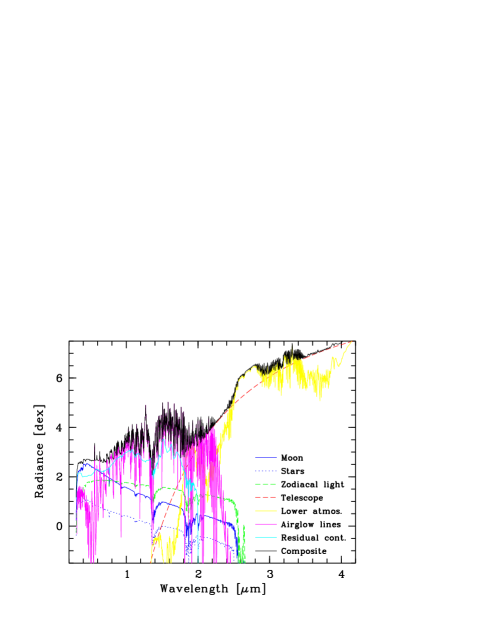
Figure 1: Components of the sky model in logarithmic radiance units for wavelengths between 0.3 and 4.2 $\mu$m. This example, with the Moon above the horizon, shows scattered moonlight, scattered starlight, zodiacal light, thermal emission by the telescope and instrument, molecular emission of the lower atmosphere, airglow emission lines of the upper atmosphere, and airglow/residual continuum. The scattered light and airglow components were only computed up to the $K$ band because of their negligible importance at longer wavelengths. For the model parameters used, see Table 1.

Due to the complexity and variability of the night-sky radiation, a good atmospheric radiation model is crucial for a reliable astronomical exposure time calculator (ETC). Currently, the European Southern Observatory (ESO) uses a sky background model for its ETC (Ballester et al. BALL00 (2000)), which includes the photometric night-sky brightness measurements of Walker (WAL87 (1987)) for the optical and Cuby et al. (CUB00 (2000)) for the near-IR. The $U$ to $I$ magnitudes of Walker vary as a function of Moon phase. For optical spectrographs, a night-sky spectrum is calculated by scaling an observed, instrument-dependent template spectrum to the Walker filter fluxes. The spectroscopic near-IR/mid-IR model is based on the line atlas of Hanuschik (HAN03 (2003)) and the OH airglow calculations of Rousselot et al. (ROU00 (2000)), thermal telescope emission, an instrument-related constant continuum, and atmospheric thermal line and continuum emission. The latter is provided as a set of template spectra computed with the radiative transfer code Reference Forward Model for different airmasses and water vapour column densities. Since the current ETC is limited in reproducing the variable intensity of the night sky, we have developed an advanced model for atmospheric radiation and transmission, which includes scattered moonlight, scattered starlight, zodiacal light, thermal emission from the telescope, molecular emission and absorption in the lower atmosphere, and airglow line and continuum emission, including their variability with time. This “sky model” has been derived for Cerro Paranal in Chile (2635 m, 24$\degr$ 38$\arcmin$ S, 70$\degr$ 24$\arcmin$ W). It is also expected to work for the nearby Cerro Armazones (3064 m, 24$\degr$ 36$\arcmin$ S, 70$\degr$ 12$\arcmin$ W), the future site of the European Extremely Large Telescope (E-ELT), without major adjustments. An example of a spectrum computed by our sky model is given in Fig. 1. The crucial input parameters are listed in Table 1. The model will be incorporated into the ESO ETC and will be made publicly available to the community via the ESO web site.

This paper focuses on the discussion of model components relevant for the wavelength range from 0.3 to 0.92 $\mu$m, which is designated as “optical” in the following. We will discuss scattering and absorption in the atmosphere (Sect. 2), contributions from extraterrestrial radiation sources (Sect. 3), and the intensity and variability of airglow emission lines and continuum (Sect. 4). The quality of our optical sky model will be evaluated in Sect. 5. The near-IR and mid-IR regimes will be treated in a subsequent paper.

If intensity units are not explicitly given in this paper, $\mathrm{photons\,\,s}^{-1}\,\mathrm{m}^{-2}\,\mu\mathrm{m}^{-1}\,\mathrm{arcsec}^{-2}$ are taken as the standard. Magnitudes are always given in the Vega system.

2 Atmospheric extinction

Light from astronomical objects is scattered and absorbed in the Earth’s atmosphere. For point sources, both effects result in a loss of radiation, which is usually described by a wavelength-dependent extinction curve or an atmospheric transmission curve. The components of such a curve for Cerro Paranal are discussed in Sect. 2.1. For extended sources, light is not only scattered out of the line of sight, it is also scattered into it. This effect causes an effective extinction curve to differ from that of a point source and depends on the spatial distribution of the extended emission. To quantify the change of the extinction curve, we performed three-dimensional (3D) scattering calculations, which are described in Sect. 2.2.

2.1 The transmission curve

The atmospheric transmission depends on scattering and absorption. Light can be scattered in dry atmosphere by air molecules such as N₂ and O₂ or by aerosols like silicate dust, sea salt, soot, or droplets of sulphuric acid. The former effect is known as Rayleigh scattering, and is characterised by a strong wavelength dependence proportional to $\lambda^{-4}$ and a relatively isotropic scattering phase function (a factor of 2 variation for unpolarised radiation). The latter can be described by Mie scattering if spherical particles are assumed. Aerosol scattering is characterised by a relatively weak wavelength dependence ($\lambda^{-1}$ to $\lambda^{-2}$) and pronounced forward scattering, for which the maximum intensity can easily be two orders of magnitude higher than at large scattering angles. Atmospheric absorption in the optical is mainly caused by bands from three molecules: molecular oxygen (O₂), water vapour (H₂O), and ozone (O₃). The absorption of O₂ is a function of atmospheric density. While water absorption is most efficient close to the ground, where the absolute humidity is the largest, ozone mainly absorbs at stratospheric altitudes of about 20 km. The combination of scattering and absorption results in an extinction curve, which is often given in mag airmass^-1, or a transmission curve providing values from 0 (totally opaque) to 1 (fully transparent). The transmission $t(\lambda)$ can be linked to the zenithal optical depth $\tau_{0}(\lambda)$ and zenithal extinction coefficient $k(\lambda)$ by

$$t(\lambda)=\mathrm{e}^{-\tau_{0}(\lambda)\,X}=10^{\,-\,0.4\,k(\lambda)\,X}.$$ (1)

The airmass $X$ can be calculated by the formula of Rozenberg (ROZ66 (1966)):

$$X=\left(\cos(z)+0.025\,\mathrm{e}^{-11\cos(z)}\right)^{-1},$$ (2)

where $z$ is the zenith distance and $X$ converges to 40 at the horizon.

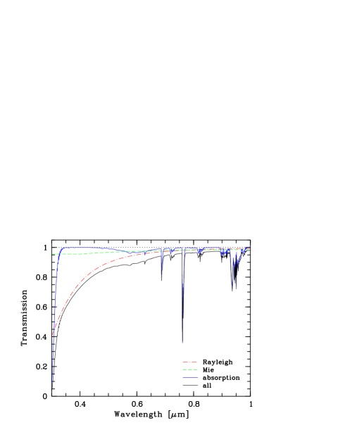
Figure 2: Annual mean zenith transmission curve for Cerro Paranal (black solid line). The Earth’s atmosphere extinguishes the flux from point sources by Rayleigh scattering by air molecules (red dash-dotted line), Mie scattering by aerosols (green dashed line), and molecular absorption (blue solid line). For the plotted wavelength range, the latter is caused by molecular oxygen (A band at 0.762 $\mu$m, B band at 0.688 $\mu$m, and $\gamma$ band at $0.628$ $\mu$m), water vapour (prominent bands at 0.72, 0.82, and 0.94 $\mu$m), and ozone (Huggins bands in the near-UV and broad Chappuis bands at about 0.6 $\mu$m).

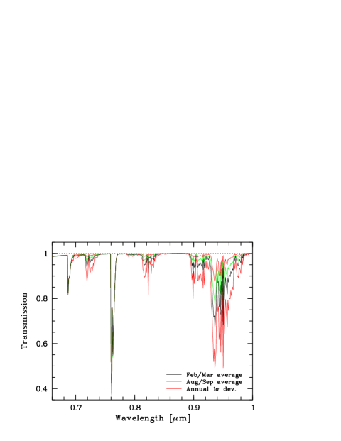
Figure 3: Variation of molecular absorption for Cerro Paranal. The extreme bimonthly mean transmission curves and 1 $\sigma$ deviations of the annual mean curve (red outer curves) are shown. The highest mean transmission (lowest water vapour content) is found for August/September (green curve), and the lowest arises in February/March (black curve). In contrast to H₂O, the variations of the O₂ bands are very small. For the identity of the bands, see Fig. 2.

For Cerro Paranal, Fig. 2 shows the annual mean transmission curve at zenith and its components. The extinction at blue wavelengths is dominated by Rayleigh scattering. This component is very stable and can be well reproduced by the parametrisation

$$\tau_{\mathrm{R}}(\lambda)=\frac{p}{1013.25}\left(0.00864+6.5\times 10^{-6}H\right)$$

$$\times\ \lambda^{\,-(3.916\,+\,0.074\,\lambda\,+\,0.050\,/\,\lambda)}$$ (3)

with wavelength $\lambda$ in $\mu$m (see Liou LIO02 (2002)). For the pressure $p$ and the height $H$, we take 744 hPa and 2.64 km respectively. The pressure corresponds to the annual mean for Cerro Paranal ($743.5\pm 1.5$ hPa), as derived from the meteorological station of the VLT Astronomical Site Monitor.

At red wavelengths, aerosol scattering becomes as important as Rayleigh scattering. However, the total amount of extinction by scattering is small in this wavelength regime. For Cerro Paranal, Patat et al. (PAT11 (2011)) provide an approximation for the aerosol extinction derived from 600 VLT FORS 1 spectra observed over six months. The aerosol extinction coefficient is parametrised by

$$k_{\mathrm{aer}}(\lambda)\approx k_{0}\,\lambda^{\,\alpha},$$ (4)

where $k_{0}=0.013\pm 0.002$ mag airmass^-1 and $\alpha=-1.38\pm 0.06$, with the wavelength $\lambda$ in $\mu$m. Due to an increased discrepancy between the fit and the observed data in the near-UV (see Patat et al. PAT11 (2011)), we use Eq. 4 only for wavelengths longer than 0.4 $\mu$m. For shorter wavelengths, we use a constant value of $k_{\mathrm{aer}}=0.050$ mag airmass^-1, which corresponds to the fit value at 0.4 $\mu$m. The density, distribution, and composition of aerosols is much more variable than what is observed for the air molecules, which determine the Rayleigh scattering. Patat et al. (PAT11 (2011)) find that $k_{\mathrm{aer}}$ varies by about 20% at 0.4 $\mu$m. However, these variations are of minor importance for the total transmission of the Earth’s atmosphere, since the aerosol extinction coefficients are small.

Figure 2 exhibits several prominent absorption bands (see also Patat et al. PAT11 (2011)). At wavelengths below 0.34 $\mu$m, there is a conspicuous fall-off of the transmission curve caused by the Huggins bands of ozone. The stratospheric ozone layer is also responsable for the Chappuis absorption bands between 0.5 and 0.7 $\mu$m. The relatively narrow, but strong, bands at 0.688 $\mu$m and 0.762 $\mu$m can be identified as the Fraunhofer B and A bands of molecular oxygen. Finally, the complex bands at 0.72, 0.82, and 0.94 $\mu$m are produced by water vapour.

The molecular absorption bands have been calculated using the Line By Line Radiative Transfer Model (LBLRTM), an atmospheric radiative transfer code provided by the Atmospheric and Environmental Research Inc. (see Clough et al. CLO05 (2005)). This widely used code in the atmospheric sciences computes transmission and radiance spectra based on the molecular line database HITRAN (see Rothman et al. ROT09 (2009)) and atmospheric vertical profiles of pressure, temperature, and abundances of relevant molecules.

For Cerro Paranal, we use merged atmospheric profiles from three data sources to reproduce the climate and weather conditions in an optimal way. First, the equatorial daytime standard profile from the MIPAS instrument of the ENVISAT satellite (prepared by J. Remedios 2001; see Seifahrt et al. SEI10 (2010)) is taken. It provides abundances for 30 molecular species up to an altitude of 120 km. Following Patat et al. (PAT11 (2011)), the ozone profile is corrected by a factor of 1.08 to achieve a column density of 258 Dobson units, which represents the mean value for Cerro Paranal. Second, we use profiles from the Global Data Assimilation System (GDAS), maintained by the Air Resources Laboratory of the National Oceanic and Atmospheric Administration (cf. Seifahrt et al. SEI10 (2010)). The GDAS profiles for pressure, temperature, and relative humidity are provided on a 3 h basis for a $1\degr\times 1\degr$ global grid. These models are adapted to data from weather stations all over the world and are suitable for weather-dependent temperature and water vapour profiles up to altitudes of 26 km. Third, data from the meteorological station at Cerro Paranal are used to scale the pressure, temperature, and water vapour profiles at the altitude of the mountain. For higher altitudes, the scaling factor is reduced and approaches 1 at 5 km.

For our sky model, we analysed the resulting data set and constructed mean profiles with their $1\,\sigma$ deviations for different periods. We divide the year into six two-month periods, starting with December/January (cf. Table 1 and Sect. 4). The two most extreme mean spectra are shown in Fig. 3. The seasonal variability of the H₂O bands is clearly visible. For the driest period (August/September), the mean absorption is only half the amount of the most humid period (February/March). The total intra-annual variability indicates line depth variations of an order of magnitude, i.e. large statistical uncertainties. For this reason, the significant seasonal dependence is included in the sky model and the less pronounced average, nocturnal variations have been neglected. Apart from the two-month period, only the airmass (see Eq. 2) is used as input parameter for the computation of transmission curves. Since radiative transfer calculations with LBLRTM are time-consuming, the sky model is run with a pre-calculated library of transmission spectra, consisting of spectra for the different bimonthly periods and a regular grid of five airmasses between 1 and 3. This is sufficient for a reliable interpolation of the airmass-dependent change of spectral features.

A more detailed discussion on atmospheric profiles, radiative transfer codes, and the properties of transmission and radiance spectra, especially in the near-IR and mid-IR, will be given in a subsequent paper.

2.2 Atmospheric scattering

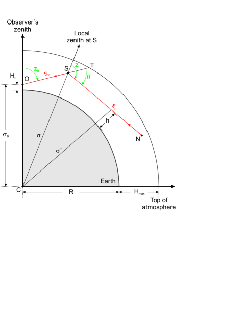
Figure 4: Geometry of the scattering in the Earth’s atmosphere (cf. Wolstencroft & van Breda WOL67 (1967)). Point $N$ is at the top of atmosphere and not in the same plane as the other points. The azimuth of $N$ as seen from $S$ is $A$ (not shown). $S$ and $T$ are at an azimuth $A_{0}$ (also not shown) for an observer at $O$.

The estimate of scattered light from extended sources, such as integrated starlight, zodiacal light, or airglow in the Earth’s atmosphere, requires radiative transfer calculations. Since the optical depth for scattering is relatively small in most of the optical wavelength range (see Fig. 2), single-scattering calculations provide a sufficient approximation. In this case, the computations can be performed in 3D with a relatively compact code (see Wolstencroft & van Breda WOL67 (1967); Staude STA75 (1975); Bernstein et al. BER02 (2002)).

To obtain the integrated scattered light towards the azimuth $A_{0}$ and zenith distance $z_{0}$, we consider scattering path elements $S$ of density $n(\sigma)$, with $\sigma$ being the radius vector from the centre of Earth $C$ to $S$, from the top of atmosphere $T$ to the observer $O$ at height $H_{0}$ above the surface (see Fig. 4). The distance of $O$ to $C$ is $\sigma_{0}=H_{0}+R$, where $R$ is the radius of Earth ($=6371$ km for the mean radius). For each path element $S$ at distance $s_{2}$ from $O$, the contributions of radiation from all directions ($A$, $z$) to the intensity at $S$ are considered. The integration over the solid angle depends on the spatial intensity distribution $I_{0}(A,z)$ of the extended radiation source and the path of the light from the entry point in the atmosphere $N$ to $S$ of length $s_{1}$. The latter includes the scattering of light out of the path (and possible absorption), which depends on the effective column density of the scattering/absorbing particles

$$B_{1}(z,\,\sigma)=\int_{0}^{s_{1}(z,\,\sigma)}n(\sigma^{\prime})\,\mathrm{d}\sigma^{\prime}.$$ (5)

It also depends on the wavelength-dependent extinction cross section $C_{\mathrm{ext}}(\lambda)$, which can be derived from the optical depth at zenith $\tau_{0}$ (see Eq. 1) by means of Eq. 5 and

$$C_{\mathrm{ext}}(\lambda)=\frac{\tau_{0}(\lambda)}{B_{0}(0,\,\sigma_{0})}.$$ (6)

After the scattering at $S$, the intensity is further reduced by the effective column density $B_{2}(z_{0},\sigma)$ along the path $s_{2}$. Thus, the calculations can be summarised by

$$I_{\mathrm{scat}}(A_{0},z_{0})=\frac{C_{\mathrm{scat}}(\lambda)}{4\pi}\int_{0}^{s_{2}(z_{0},\,\sigma_{0})}\int_{0}^{z_{\mathrm{max}}(\sigma)}\int_{0}^{2\pi}n(\sigma)\,P(\theta)$$

$$\times\ I_{0}(A,z)\,\mathrm{e}^{-C_{\mathrm{ext}}(\lambda)\left[B_{1}(z,\,\sigma)+B_{2}(z_{0},\,\sigma)\right]}\,\mathrm{d}A\,\sin z\,\mathrm{d}z\,\mathrm{d}s.$$ (7)

$C_{\mathrm{scat}}$ is the wavelength-dependent scattering cross section, which will deviate from $C_{\mathrm{ext}}$ if absorption occurs. The maximum zenith distance $z_{\mathrm{max}}$ is higher than $90\degr$ and depends on the height of $S$ above the ground. The scattering phase function $P$ depends on the scattering angle $\theta$, the angle between the paths $s_{1}$ and $s_{2}$.

Rayleigh scattering (see Sect. 2.1) is characterised by the phase function

$$P(\theta)=\frac{3}{4}\left(1+\cos^{2}(\theta)\right).$$ (8)

Similar to Bernstein et al. (BER02 (2002)), we neglect the effect of polarisation on the scattering phase function. Even for zodiacal light, where some polarisation is expected (e.g. Staude STA75 (1975)), the polarisation does not appear to significantly affect the integrated scattered light. Results of Wolstencroft & van Breda (WOL67 (1967)) suggest deviations of only a few per cent. For the vertical distribution of the scattering molecules, we use the standard barometric formula

$$n(h)=n_{0}\,\mathrm{e}^{-h/h_{0}}.$$ (9)

Here, $h=\sigma^{\prime}-R$, the sea level density $n_{0}=2.67\times 10^{19}$ cm^-3, and the scale height $h_{0}=7.99$ km above the Earth’s surface (cf. Bernstein et al. BER02 (2002)). For the troposphere and the lower stratosphere, where most of the scattering occurs, this is a good approximation. Cerro Paranal is at an altitude of $H_{0}=2.64$ km. For the thickness of the atmosphere, we take $H_{\mathrm{max}}=200$ km. With these values, $C_{\mathrm{ext}}$ is $1.75\times 10^{-26}$ cm² for $\tau_{0}=0.27$, which corresponds to a wavelength of about 0.4 $\mu$m. For Rayleigh scattering, $C_{\mathrm{scat}}=C_{\mathrm{ext}}$, i.e. no absorption is involved. In the near-UV, where the zenithal optical depth is greater than 0.3, the single scattering approximation becomes questionable. For this reason, we apply a multiple scattering correction derived from radiative transfer calculations in a plane-parallel atmosphere (see Dave DAV64 (1964); Staude STA75 (1975)). We multiply $I_{\mathrm{scat}}$ by the factor

$$F_{\mathrm{MS}}=1+2.2\,\tau_{0}.$$ (10)

The uncertainty is in the order of 5%. The factor $F_{\mathrm{MS}}$ does not include reflection from the ground. Mattila (MAT03 (2003)) reports a ground reflectance of about 8% in the region near the Las Campanas Observatory in autumn. Since this telescope site is also located in the Atacama desert, we assume this value with an uncertainty of a few per cent. Using the tables of Ashburn (ASH54 (1954)), an 8% reflectance translates into an additional $I_{\mathrm{scat}}$ correction factor of about 1.07.

The Mie scattering of aerosols is characterised by a phase function with a strong peak in forward direction. For this study, we take the measured $P(\theta)$ of Green et al. (GRE71 (1971)), which covers the peak up to an angle of $20\degr$. The phase function for larger scattering angles is extrapolated by a linear fit in the $\log P-\log\theta$ diagram. This simple approach neglects the increase of the phase function for scattering angles close to $180\degr$ (see e.g. Liou LIO02 (2002)). However, since $P$ already decreases by a factor of 30 from $0\degr$ to $20\degr$, the details of the phase function at larger angles are not crucial for the scattering of extended emission. The total scattered intensity is completely dominated by the contribution from angles close to the forward direction. For the height distribution of aerosols, we also take Eq. 9, but assume $n_{0}=1.11\times 10^{4}$ cm^-3 and $h_{0}=1.2$ km. This is the tropospherical distribution of Elterman (ELT66 (1966)). Following Staude (STA75 (1975)), we neglect the stratospheric aerosol component, which contains only about 1% of the particles. Using Eq. 6 we obtain $C_{\mathrm{ext}}=3.39\times 10^{-10}$ cm² for $\tau_{0}=0.05$, which characterises wavelengths of about 0.4 $\mu$m. Dust, in particular soot, also absorbs radiation. For this reason, $C_{\mathrm{scat}}$ is lower than $C_{\mathrm{ext}}$. The ratio of these is called the single scattering albedo $\tilde{\omega}$. Following the recommendation of Mattila (MAT03 (2003)), $\tilde{\omega}=0.94$ is used for the model, i.e. strong absorbers like soot do not significantly contribute to the aerosol population. We neglect any corrections for multiple scattering and ground reflection for Mie scattering, since the optical depths are low at all relevant wavelengths (see Fig. 2) and forward scattering dominates.

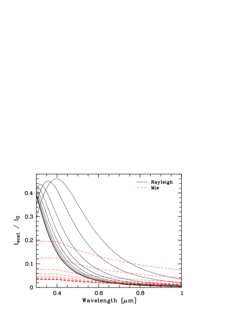
Figure 5: Intensity of scattered radiation for a uniform source of unit brightness using the Paranal extinction curve (see Sect. 2.1). Contributions of scattered light into the line of sight are shown for Rayleigh (solid lines) and Mie scattering (dashed lines) and zenith distances from 0$\degr$ to 80$\degr$ in 10$\degr$ steps plus an extreme value of 85$\degr$. Except for Rayleigh scattering at very short wavelengths, the scattering intensities increase with zenith distance.

To test our model, we computed scattering intensities for a uniform radiation source of unit brightness. For the surface level and $\tau_{0}=0.052$, we obtain scattering fractions of $0.024$ for the zenith and $0.360$ for the horizon ($z_{0}=90\degr$) with the multiple scattering corrections neglected. For Rayleigh scattering, these results can be compared to those of Staude (STA75 (1975)). Our values are only about 5% higher. This is a good agreement compared to differences between Staude (STA75 (1975)) and older calculations of Wolstencroft & van Breda (WOL67 (1967)) and Ashburn (ASH54 (1954)). Figure 5 shows the resulting scattering fractions for Rayleigh and Mie scattering for different optical depths, which have been converted into wavelengths based on the Cerro Paranal mean transmission curve discussed in Sect. 2.1. For zenith distances that are realistic for astronomical observations, wavelengths longer than about $0.45$ $\mu$m for Rayleigh scattering, and all wavelengths for aerosol scattering, the scattering fractions stay below 10% for a source of uniform brightness. Scattering by air molecules and the ground surface can be important for lines of sight close to the horizon and near-UV wavelengths. Figure 5 indicates scattering fractions of about 40% under these conditions. Moreover, there appears to be a downturn of the scattering fraction for very high zenith distances (see also Staude STA75 (1975)), where the line-of-sight direction becomes nearly opaque. In this case, the light that is not extinguished has to be scattered near the observer and the incident photons have to originate close to the zenith.

The results of scattering calculations for more realistic source intensity distributions will be discussed in Sects. 3.2, 3.3, and 4.3.

3 Moon, stars, and interplanetary dust

Bright astronomical objects affect night-sky observations by the scattering of their radiation into the line of sight. The relevant initial radiation sources are the Sun and the summed-up light of all other stars. The solar radiation must first be scattered by interplanetary dust grains and the Moon surface to contribute to the night-sky brightness. In the following, we discuss these scattering-related sky model components, i.e. scattered moonlight (Sect. 3.1), scattered starlight (Sect. 3.2), and zodiacal light (Sect. 3.3). Another source of scattered light is man-made light pollution, which can be neglected for Cerro Paranal. Patat (PAT03 (2003)) did not detect spectroscopic signatures of such contamination.

3.1 Scattered moonlight

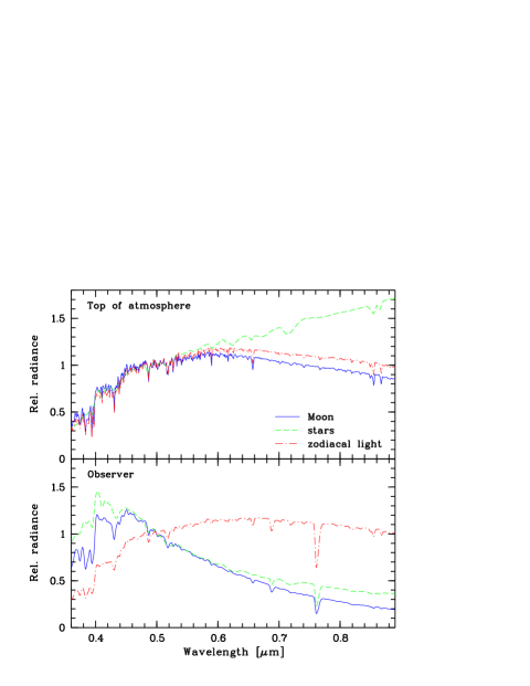
Figure 6: Effects of atmospheric scattering on radiation originating outside of the atmosphere. The displayed radiation sources are Moon (blue solid lines), stars (green dashed lines), and interplanetary dust (red dash-dotted lines). All spectra are normalised to unity at 0.5 $\mu$m. In the upper panel, a solar spectrum is assumed as top-of-atmosphere spectrum for moonlight (see Sect. 3.1). A slightly reddened solar spectrum is taken for solar radiation scattered at interplanetary dust grains (see Sect. 3.3). Integrated starlight tends to be redder than sunlight at long wavelengths (see Sect. 3.2). The lower panel shows the resulting low-resolution spectra, after light has been scattered in the Earth’s atmosphere, for observing conditions as listed in Table 1. While the lunar and stellar contributions represent scattered radiation only, the dust-related zodiacal light consists of scattered and direct light.

For observing dates close to Full Moon, scattered moonlight is by far the brightest component of the optical night-sky background. In particular, blue wavelengths are affected, since the Moon spectrum resembles a solar spectrum and the efficency of Rayleigh/Mie scattering increases towards shorter wavelengths (see Fig. 2).

The Moon can be considered a point source. For this reason, it is not necessary to perform the scattering calculations for extended sources, as discussed in Sect. 2.2. Instead, a semi-analytical model for the photometric $V$ band by Krisciunas & Schaefer (KRI91 (1991)) is used for the sky model, which has been extended into a spectroscopic version.

Based on Krisciunas & Schaefer (KRI91 (1991)), we compute the Moon-related sky surface brightness as the sum of the contributions from Rayleigh and Mie scattering

$$B_{\mathrm{moon}}(\lambda)=B_{\mathrm{moon,R}}(\lambda)+B_{\mathrm{moon,M}}(\lambda),$$ (11)

where

$$B_{\mathrm{moon,R/M}}(\lambda)=f_{\mathrm{R/M}}(\rho)\,I^{*}(\lambda)\,t^{\,X_{\mathrm{moon}}}(\lambda)\,(1-t_{\mathrm{R/M}}^{\,X_{0}}(\lambda)).$$ (12)

The empirical scattering functions

$$f_{\mathrm{R}}(\rho)=10^{\,5.70}\left(1.06+\cos^{2}(\rho)\right)$$ (13)

for Rayleigh scattering and

$$f_{\mathrm{M}}(\rho)=10^{\,7.15\,-\,(\rho/40)}$$ (14)

for Mie scattering depend on the angular separation of Moon and object $\rho$, which is restricted to angles greater than $10\degr$. The functions deviate from the ones of Krisciunas & Schaefer (KRI91 (1991)) by factors of 2.2 and 10 respectively. These corrections are necessary because of the separation of the two scattering processes in Eqs. 11 and 12, the model extension in wavelength, and an optimisation for the observing conditions at Cerro Paranal. The two correction factors were derived separately from a comparison with optical VLT data (see Sect. 4.2) by using the increasing importance of Rayleigh scattering with respect to Mie scattering for shorter wavelengths and larger scattering angles $\rho$ (see Sect. 2.2). The factor of 10 for Mie scattering is highly uncertain due to a lack of clear constraints from the available data set. The Moon illuminance is proportional to

$$I^{*}\propto 10^{\,-\,0.4\,(0.026\,|\phi|\,+\,4.0\,\times\,10^{-9}\,\phi^{4})}\times\left(d_{\mathrm{moon}}\right)^{-2},$$ (15)

where the Moon distance $d_{\mathrm{moon}}$ can vary up to 5.5% relative to the mean value. The lunar phase angle $\alpha=180\degr-\phi$ is the separation angle of Moon and Sun as seen from Earth. It can be estimated from the fractional lunar illumination (FLI) by

$$\alpha\approx\arccos(1-2\,\mathrm{FLI}),$$ (16)

since the influence of the lunar ecliptic latitude on $\alpha$ is negligible. $B_{\mathrm{moon}}$ also depends on the atmospheric transmission for the airmass of the Moon $t^{\,X_{\mathrm{moon}}}$, for which the Patat et al. (PAT11 (2011)) extinction curve is used (see Fig. 2). Lastly, it depends on a term that describes the amount of scattered moonlight in the viewing direction, which can be roughly approximated by $1-t_{\mathrm{R/M}}^{\,X_{0}}$ for either Rayleigh or Mie scattering and the target airmass $X_{0}$. The airmasses of the Krisciunas & Schaefer (KRI91 (1991)) model are computed using

$$X=\left(1-0.96\sin^{2}(z)\right)^{-0.5},$$ (17)

which is especially suited for scattered light, because of a low limiting airmass at the horizon (cf. Eq. 2).

The Krisciunas & Schaefer model was developed only for the $V$ band. It can be extended to other wavelength ranges by using the Cerro Paranal extinction curve (see Sect. 2.1) and its Rayleigh and Mie components for the transmission curves $t$, $t_{\mathrm{R}}$, and $t_{\mathrm{M}}$ in Eq. 12 and by assuming that the Moon spectrum resembles the spectrum of the Sun (see Fig. 6). The latter is modelled by the solar spectrum of Colina et al. (COL96 (1996)) scaled to the $V$-band brightness of the moonlight scattering model. For most situations, this approach results in systematic uncertainties of no more than 10% of the total night-sky flux compared to observations. The statistical uncertainties are in the order of 10 to 20% (see Sect. 5). The errors become larger for Full Moon and/or target positions close to the Moon ($\rho\la 30\degr$). The latter especially concerns red wavelengths, where the contribution of Mie forward scattering to the total intensity of scattered light is particularly high. Consequently, the strongly varying aerosol properties have to be known (which is a challenging task) to allow for a good agreement of model and observations. However, optical astronomical observations close to the Moon are unlikely. Therefore, this is not a critical issue for the sky model.

3.2 Scattered starlight

Like moonlight, starlight is also scattered in the Earth’s atmosphere. However, stars are distributed over the entire sky with a distribution maximum towards the centre of the Milky Way. This distribution requires the use of the scattering model for extended sources described in Sect. 2.2. Since scattered starlight is only a minor component compared to scattered moonlight and zodiacal light (see Fig. 1), it is sufficient for an ETC application to compute a mean spectrum. This simplification allows us to avoid the introduction of sky model parameters such as the galactic coordinates, which have a very low impact on the total model flux.

For the integrated starlight (ISL), we use Pioneer 10 data at 0.44 $\mu$m (Toller TOL81 (1981); Toller et al. TOL87 (1987); Leinert et al. LEI98 (1998)). These data are almost unaffected by zodiacal light. The small “hole” in the data set towards the Sun has been filled by interpolation. Since the Pioneer 10 maps do not include stars brighter than 6.5 mag in $V$, a global correction given by Melchior et al. (MEL07 (2007)) is applied, which increases the total flux by about 16%. Scattering calculations are only performed for the distribution of starlight in the $B$ band, i.e. the dependence of this distribution on wavelength is neglected. This approach is supported by calculations of Bernstein et al. (BER02 (2002)), indicating that the shapes of ISL spectra are very stable, except for regions in the dustiest parts of the Milky Way plane. The wavelength dependence of the scattered starlight is considered by multiplying the representative ISL mean spectrum of Mattila (MAT80 (1980)) by the resulting wavelength-dependent amount of scattered light (for illustration see Figs. 5 and 6). Since the mean ISL spectrum of Mattila only covers wavelengths up to 1 $\mu$m, we extrapolated the spectral range by fitting an average of typical spectral energy distributions (SED) for early- and late-type galaxies produced by the SED-fitting code CIGALE (see Noll et al. NOL09 (2009)). Since the SED slopes are very similar in the near-IR, the choice of the spectral type is not crucial. The solar and the mean ISL spectrum are similar at blue wavelengths, but the ISL spectrum has a redder slope at longer wavelengths (see Fig. 6). The differences illustrate the importance of K and M stars for the ISL.

For the desired average scattered light spectrum, we run our scattering code for different combinations of zenithal optical depth, zenith distance, azimuth, and sidereal time for Rayleigh and Mie scattering (see Sect. 2.2). The step sizes for the latter three parameters were $10\degr$, $45\degr$, and 2 h, respectively. Zenith distances were only calculated up to $50\degr$, since this results in a mean airmass of about $1.25$ for the covered solid angle, which is typical of astronomical observations. The mean scattering intensities for each optical depth $\tau_{0}$ were then computed. This was translated into a spectrum by using the relation between $\tau_{0}$ and wavelength as provided by the Cerro Paranal extinction curve (see Sect. 2.1). Finally, the mean ISL spectrum (normalised to the $B$-band flux) was multiplied. The sky model code does not change the final spectrum, except for the molecular absorption, which is adjusted depending on the bimonthly period (see Sect. 2.1). For the effective absorption airmass, the mean value of $1.25$ is assumed.

The resulting spectrum shows an intensity of about 13 $\mathrm{photons\,\,s}^{-1}\,\mathrm{m}^{-2}\,\mu\mathrm{m}^{-1}\,\mathrm{arcsec}^{-2}$ at 0.4 $\mu$m. At $0.6$ $\mu$m, there is only half of this intensity (see Fig. 6). The results are in good agreement with the findings of Bernstein et al. (BER02 (2002)).

3.3 Zodiacal light

Zodiacal light is caused by scattered sunlight from interplanetary dust grains in the plane of the ecliptic. A strong contribution is found for low absolute values of ecliptic latitude $\beta$ and heliocentric ecliptic longitude $\lambda-\lambda_{\sun}$. The brightness distribution provided by Levasseur-Regourd & Dumont (LEV80 (1980)) and Leinert et al. (LEI98 (1998)) for $0.5$ $\mu$m shows a relatively smooth decrease for increasing elongation, i.e. angular separation of object and Sun. A striking exception is the local maximum of the so-called gegenschein at the antisolar point in the ecliptic. The spectrum of the optical zodical light is similar to the solar spectrum (Colina et al. COL96 (1996)), but slightly reddened (see Fig. 6). We apply the relations given in Leinert et al. (LEI98 (1998)) to account for the reddening. The correction is larger for smaller elongations. Thermal emission of interplanetary dust grains in the IR is neglected in the sky model, since the airglow components of atmospheric origin (see Fig. 1) completely outshine it. In the optical, zodiacal light is a significant component of the sky model. A contribution of about 50% is typical of the $B$ and $V$ bands when the Moon is down (see Sect. 5.2). At longer wavelengths, the fraction decreases due to the increasing importance of the airglow continuum (see Sect. 4.4).

The model of the zodiacal light presented in Leinert et al. (LEI98 (1998)) describes the characteristics of this emission component outside of the Earth’s atmosphere. Ground-based observations of the zodical light also have to take atmospheric extinction into account. Since zodiacal light is an extended radiation source, the observed intensity is a combination of the extinguished top-of-atmosphere emission in the viewing direction and the intensity of light scattered into the line of sight (see Fig. 6). The latter can be treated by scattering calculations as discussed in Sect. 2.2. Scattering out of and into the line of sight leads to an effective extinction and this can be expressed by an effective optical depth

$$\tau_{\mathrm{eff}}=\tau_{\mathrm{0,eff}}\,X=f_{\mathrm{ext}}\,\tau_{0}\,X$$ (18)

(cf. Eq. 1; see also Bernstein et al. BER02 (2002)). Consequently, the scattering properties of the zodiacal light can be described by the factor $f_{\mathrm{ext}}$ alone. This parameter shows only a weak dependence on $\tau_{0}$ and, hence, wavelength. For Rayleigh scattering in the range from $U$ to $I$ band, we find an uncertainty of only about 4%. For Mie scattering from $V$ to $J$, a similar variation is found. We obtain this result by calculating $f_{\mathrm{ext}}$ for a grid of optical depths, zenith distances, azimuths, sideral times, and solar ecliptic longitudes. We take the same grid as for scattered starlight (see Sect. 3.2) plus solar ecliptic longitudes in steps of $90\degr$, i.e. for each of the four seasons, one data set was calculated. Scattering calculations were only carried out for solar zenith distances of at least $108\degr$. This restriction excludes daytime and twilight conditions. As for scattered starlight, we consider target zenith distances $z$ up to $50\degr$ (see Sect. 3.2). For rare high zodiacal light intensities, we also let $50\degr<z\leq 70\degr$. The $z$ limits do not significantly affect $f_{\mathrm{ext}}$. A test with $0\degr\leq z\leq 70\degr$ showed a variation of $f_{\mathrm{ext}}$ in the order of a few per cent only.

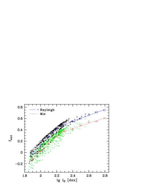
Figure 7: Extinction reduction factor $f_{\mathrm{ext}}$ for zodiacal light as a function of the line-of-sight top-of-atmosphere intensity $I_{0}$ of the zodiacal light in dex. The intensities correpond to those given in Table 17 of Leinert et al. (LEI98 (1998)), i.e. the unit is $10^{-8}\,\mathrm{W\,m}^{-2}\,\mu\mathrm{m}^{-1}\,\mathrm{sr}^{-1}$ ($=1.690$ $\mathrm{photons\,\,s}^{-1}\,\mathrm{m}^{-2}\,\mu\mathrm{m}^{-1}\,\mathrm{arcsec}^{-2}$ at 0.5 $\mu$m). The factors were calculated for different ecliptic longitudes of the Sun, sidereal times, and line-of-sight zenith distances (up to 50$\degr$ in general and up to 70$\degr$ for $\log I_{0}>2.4$) and azimuths. Only night-time data points with solar zenith distances greater than 108$\degr$ are considered. For Rayleigh scattering (black ’x’ symbols), a zenithal optical depth of 0.27 is taken, corresponding to a wavelength of 0.4 $\mu$m for the Cerro Paranal extinction curve (see Sect. 2.1). For Mie scattering (green ’+’ symbols), $\tau_{0}$ is fixed to 0.01, a value reached at about 1.2 $\mu$m. The figure also shows average $f_{\mathrm{ext}}$ in 0.1 dex $I_{0}$ bins for both scattering modes (Rayleigh: blue circles; Mie: red triangles). The resulting fits based on these average values are displayed by solid (Rayleigh) and dashed lines (Mie).

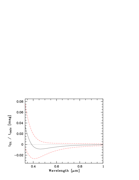
Figure 8: Ratio of the zodiacal light transmissions of the fits as shown in Fig. 7 and the full scattering calculations in magnitudes. The wavelength-dependent mean values and 1 $\sigma$ deviations are displayed as solid and dashed lines respectively.

For an efficient implementation in the ETC, we searched for a parametrisation of $f_{\mathrm{ext}}$ that simplifies the treatment of scattering and minimises the number of required input parameters. We found that the intial intensity of the zodiacal light in the viewing direction $I_{0}$ indicates the tightest relation with $f_{\mathrm{ext}}$. The next-best parameter is the ecliptic latitude. Figure 7 shows $f_{\mathrm{ext}}$ versus the logarithm of $I_{0}$ as provided by Leinert et al. (LEI98 (1998)) for Rayleigh and Mie scattering. Since the variation of $f_{\mathrm{ext}}$ with $\tau_{0}$ can be neglected, the optical depth is fixed to $0.27$ for Rayleigh and $0.01$ for Mie scattering. These values correspond to the wavelengths $0.4$ and $1.2$ $\mu$m respectively, which represent typical wavelengths dominated by the two different scattering processes (see Fig. 2). The distribution of data points in Fig. 7 exhibits a clear increase of $f_{\mathrm{ext}}$ with $I_{0}$. The slopes appear to be very similar for both scattering processes. The extinction reduction factor $f_{\mathrm{ext,M}}$ for Mie scattering tends to be about 0.1 lower than $f_{\mathrm{ext,R}}$ for Rayleigh scattering. The difference increases with increasing $I_{0}$. For very low zodiacal light intensities in the viewing direction, $f_{\mathrm{ext}}$ becomes negative. Here, the scattering of light from directions of high zodiacal light brightness into the line of sight overcompensates the extinction. For viewing directions with higher $I_{0}$, this process is less effective and causes higher $f_{\mathrm{ext}}$. The investigated parameter space does not indicate values higher than about 0.75, i.e. the zodiacal light in the direction of astronomical observing targets is always significantly less attenuated in the Earth’s atmosphere than a point source (cf. Leinert et al. LEI98 (1998)).

The good correlation of $f_{\mathrm{ext}}$ and $I_{0}$ allows us to describe the reduction of the optical depth with $I_{0}$ only. The unextinguished zodiacal light is derived from the ecliptic coordinates, which are given sky model parameters (see Table 1). Figure 7 displays the resulting linear fits to the data based on average $f_{\mathrm{ext}}$ for 0.1 dex bins of $\log I_{0}$. The parameters obtained by these split fits are

$$f_{\mathrm{ext,R}}=\begin{cases}1.407\log I_{0}-2.692&\text{if }\log I_{0}\leq 2.244,\\ 0.527\log I_{0}-0.715&\text{if }\log I_{0}>2.244\\ \end{cases}$$ (19)

for Rayleigh scattering and

$$f_{\mathrm{ext,M}}=\begin{cases}1.309\log I_{0}-2.598&\text{if }\log I_{0}\leq 2.255,\\ 0.468\log I_{0}-0.702&\text{if }\log I_{0}>2.255\\ \end{cases}$$ (20)

for Mie scattering with $I_{0}$ in $10^{-8}\,\mathrm{W\,m}^{-2}\,\mu\mathrm{m}^{-1}\,\mathrm{sr}^{-1}$. For the fits of the lower $I_{0}$, the $f_{\mathrm{ext}}$ standard deviations of the data from the regression lines are 0.06 and 0.07 for Rayleigh and Mie scattering respectively. For the higher $I_{0}$, systematic uncertainties are probably higher than statistical variations, since these values are rare when $z\leq 70\degr$ and $z_{\,\sun}\geq 108\degr$.

The quality of the parametrisation in Eqs. 19 and 20 is illustrated by Fig. 8, which shows the average ratio of the fitted and originally calculated transmission for the entire parameter grid as derived from Eqs. 1 and 18 in magnitudes. In almost the entire wavelength range, the accuracy of the mean is better than 1%. Only at very short wavelengths, the systematic errors become higher. The intersection of the zero line at about $0.4$ $\mu$m is caused by the selection of $\tau_{0}=0.27$ for the $f_{\mathrm{ext,R}}$ fitting. The $1\sigma$ range suggests uncertainties of no more than 3 to 4% for most wavelengths. These results suggest that the parametrisation of $\tau_{\mathrm{eff}}$ does not cause higher errors than those expected from the uncertainties of the scattering calculations (see Sect. 2.2). The total errors from the simple treatment of multiple scattering and ground reflection, neglection of polarisation, simplified particle distributions, and uncertainties in the aerosol scattering parameters should be in the order of 10% of $I_{\mathrm{scat}}$. This translates into uncertainties in the transmission of a few per cent at blue wavelengths, which is somewhat higher than the uncertainties from the $f_{\mathrm{ext}}$ fit.

Finally, the reduction of the zodiacal light intensity by molecular absorption has to be considered. Strong absorption is only important for relatively long wavelengths, where scattering affects only a few per cent of the incoming light (see Fig. 2), assuming zenith distances of typical astronomical observations. Hence, the direct component in the viewing direction is usually much brighter than the scattered light from other directions. For this reason, we can safely assume that the target airmass is well suited to derive the transmission reduction by molecular absorption. Differences between target and effective scattering airmasses can be neglected.

4 Airglow emission

Atmospheric emission at wavelengths from the near-UV to the near-IR originates in the upper atmosphere, especially in the mesopause region at an altitude of about 90 km and in the ionospheric F2 layer at about 270 km. In contrast to the thermal radiation in the mid-IR by atmospheric greenhouse gases in the lower atmosphere, this so-called airglow (see Khomich et al. KHO08 (2008) for a comprehensive discussion) is caused by a highly non-LTE emission process called chemiluminescence, i.e. by chemical reactions that lead to light emission by the decay of excited electronic states of reaction products. Consequently, atmospheric radiative transfer codes like LBLRTM (Clough et al. CLO05 (2005); see also Sect. 2.1) cannot be used to calculate this emission. Moreover, theoretical analysis is very challenging because of the high variability of airglow on various time scales. The complex reactions are affected by the varying densities of the involved molecules, atoms, and ions in different excitation states. Therefore, airglow can best be treated by a semi-empirical approach. The section starts with a general discussion of airglow extinction (Sect. 4.1). In Sect. 4.2, we present the data set that was used to derive the model. Detailed discussions of the line and continuum components of the model can be found in Sects. 4.3 and 4.4 respectively.

4.1 Extinction of airglow emission

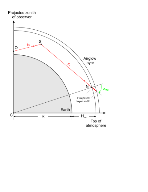
Figure 9: Illustration of the projected emission layer width used for the derivation of the beam-specific, incident airglow intensities in the 3D scattering calculations. The extension of the scattering atmosphere is limited to the lower boundary of the airglow emission layer. Point $O$ can be in a different plane from the other points (cf. Fig. 4).

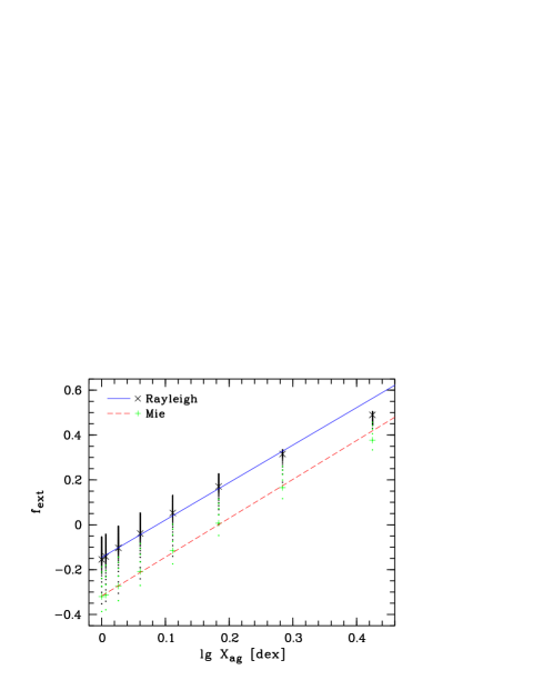
Figure 10: Extinction reduction factor $f_{\mathrm{ext}}$ for airglow as a function of airmass (see Eq. 23) in dex. The factors were calculated for different line-of-sight zenith distances $z$ (in 10$\degr$ steps) and zenithal optical depths $\tau_{0}$. For Rayleigh ($\tau_{0}\leq 0.99$) and Mie scattering ($\tau_{0}\leq 0.05$), the values for $\tau_{0}=0.27$ and $0.01$ are marked by black ’x’ and green ’+’ symbols respectively. For $z\leq 60\degr$, these values were used to derive airmass-dependent relations for $f_{\mathrm{ext}}$. The resulting fits are displayed by blue solid (Rayleigh) and red dashed lines (Mie).

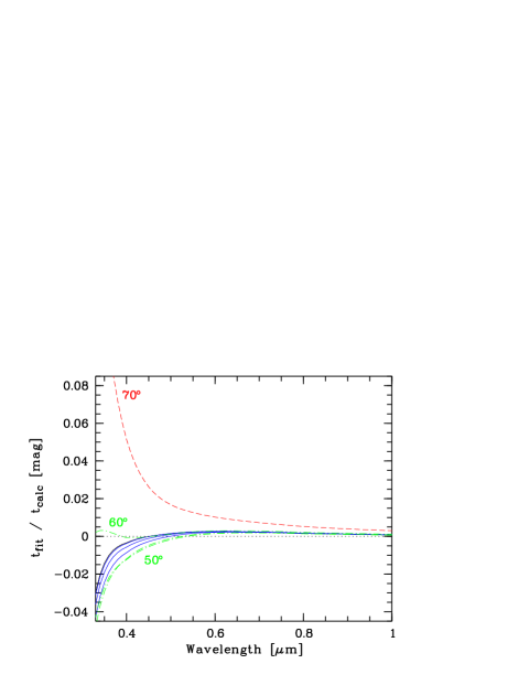
Figure 11: Ratio of the airglow transmissions of the fits as shown in Fig. 10 and the full scattering calculations in magnitudes. The wavelength-dependent results for line-of-sight zenith distances from 0$\degr$ (black solid line) to 70$\degr$ (red dashed line) in 10$\degr$ steps are exhibited.

The intensities of airglow lines and continuum rise with growing zenith distance by the increase of the projected emission layer width. This behaviour is expressed by the van Rhijn function

$$\frac{I(z)}{I(0)}=\left(1-\left(\frac{R\sin(z)}{R+h}\right)^{2}\right)^{-0.5}$$ (21)

(van Rhijn RHI21 (1921)). Here, $z$, $R$, and $h$ are the zenith distance, the Earth’s radius, and the height of the emitting layer above the Earth’s surface (see Table 2), respectively. The airglow intensity is also affected by scattering and absorption in the lower atmosphere. Since the airglow emission is distributed over the entire sky, we can derive the effective extinction by means of scattering calculations as described in Sect. 2.2. Some modifications have to be applied, since airglow emission originates in the atmosphere itself and because of the van Rhijn effect. The top of atmosphere is reduced from the default $H_{\mathrm{max}}=200$ km to 90 km, which is assumed to be representative of airglow emission layers. The few atomic lines originating in the ionospheric F2 layer are neglected here (see Sect. 4.3). The cut at the lower height is not critical, since the mass of the excluded range is negligible compared to the total mass of the atmosphere (see Eq. 9). The projected emission layer width (see Fig. 9) is considered by calculating the zenith distance $z_{\mathrm{\,ag}}$ of each incoming beam as seen from the corresponding entry point $N$ at $H_{\mathrm{max}}$. For our set-up, the resulting beam-specific airglow intensity can be approximated by

$$I(z_{\mathrm{\,ag}})=\frac{I_{0}}{\cos(z_{\mathrm{\,ag}})},$$ (22)

since the centres of the scattering path elements $S$ are always located well below the airglow emission layer height, which avoids $z_{\mathrm{\,ag}}=90\degr$. The intensity $I_{0}$ for a perpendicular incidence at $N$ is assumed to be constant for the entire global airglow layer. The scattering calculations only depend on the zenithal optical depth and the target zenith distance.

Like for the zodiacal light (see Sect. 3.3), we can derive an optical depth reduction factor $f_{\mathrm{ext}}$ (Eq. 18) to describe the airglow extinction properties. The representative optical depths are again 0.27 for Rayleigh scattering (6% uncertainty from $U$ to $I$ band) and 0.01 for Mie scattering (4% variation from $V$ to $J$ band). The only remaining free parameter for $f_{\mathrm{ext}}$ is the zenith distance or airmass. We take

$$X_{\mathrm{\,ag}}=\left(1-0.972\sin^{2}(z)\right)^{-0.5}$$ (23)

(cf. Eq. 17), which corresponds to the van Rhijn formula (Eq. 21) for the assumed airglow layer height of 90 km. $X_{\mathrm{\,ag}}$ is better suited for fitting $f_{\mathrm{ext}}$ and Eq. 18 than the Rozenberg (ROZ66 (1966)) airmass $X$ (Eq. 2) used for the zodiacal light (see Sect. 3.3), where the $z$ dependence of $f_{\mathrm{ext}}$ was negligible. Figure 10 shows the extinction reduction factor as a function of the logarithm of $X_{\mathrm{\,ag}}$. There is a strong increase in $f_{\mathrm{ext}}$ with airmass, and the factors for the Mie scattering tend to be about $0.15$ lower than those for Rayleigh scattering. These trends are in good agreement with our findings for the zodiacal light. However, the typical values of $f_{\mathrm{ext}}$ are significantly lower. For most zenith distances relevant for astronomical observations, the factors are close to zero. Consequently, the effective extinction of airglow is very low (see Chamberlain CHA61 (1961)). For observations close to zenith, there is even a significant brightening of the airglow emission by the scattering into the line of sight from light with a long path length through the emission layer. Therefore, using a point-source transmission curve for airglow extinction correction will provide worse results than having no correction. As indicated by Fig. 10, a rough correction of airglow emission using the van Rhijn equation is reasonable up to zenith distances of $50\degr$ to $60\degr$, depending on the ratio of Rayleigh and Mie scattering. At higher zenith distances, the compensation of extinction of direct light by scattered light from other directions becomes less efficient. At the largest $z$, the intensity can be more reduced by extinction than enhanced by the van Rhijn effect. For this reason, there is a zenith distance with a maximum airglow intensity, which depends on the optical depth and, hence, the wavelength. For the Cerro Paranal extinction curve (see Sect. 2.1), we found a $z_{\mathrm{max}}$ of about $70\degr$ at $0.35$ $\mu$m and $85\degr$ at $0.7$ $\mu$m.

For the sky model, $f_{\mathrm{ext}}$ was fit up to a zenith distance of $60\degr$, where $f_{\mathrm{ext}}$ shows an almost linear relation with the logarithm of $X_{\mathrm{\,ag}}$ (see Fig. 10). A worse agreement at large zenith distances is tolerable, since astronomical observations are rarely carried out at those angles. The parameters obtained by the fits are

$$f_{\mathrm{ext,R}}=1.669\log X_{\mathrm{\,ag}}-0.146$$ (24)

for Rayleigh scattering and

$$f_{\mathrm{ext,M}}=1.732\log X_{\mathrm{\,ag}}-0.318$$ (25)

for Mie scattering. For the fixed optical depths and the fitted $z$ range, the fit uncertainties of $f_{\mathrm{ext}}$ are only about 0.01. Figure 11 displays the accuracy of the fits as a function of wavelength. For this plot, the Cerro Paranal extinction curve (see Sect. 2.1) was used to convert optical depths into wavelengths. For the fitted range of zenith distances, the deviations between fitted and the true transmission curves are below 1%, at least for wavelengths longer than $0.4$ $\mu$m. As expected, the deviations for $z=70\degr$ are significantly larger than for the smaller zenith distances. Nevertheless, for most prominent airglow lines (see Sect. 4.3), the errors are below 2%, which also makes the parametrisation sufficient for large zenith distances.

Apart from scattering, molecular absorption in the lower atmosphere affects the observed airglow intensity. However, in the optical these absorptions are usually small (see Fig. 2). Exceptions are the airglow O₂(b-X)(0-0) and O₂(b-X)(1-0) bands at 762 and 688 nm, which suffer from heavy self-absorption at low altitudes, and can be observed as absorption bands only. As discussed in Sect. 3.3, the effective molecular absorption can be well approximated by taking the transmission spectrum for the target zenith distance. For the airglow continuum component, this is easily applied. For the line component, this is challenging, since airglow emission as well as telluric absorption lines are very narrow. Therefore, an effective absorption for each airglow line has to be derived at very high resolution. Resolving the airglow lines requires resolutions in the order of $10^{6}$. The absorption lines tend to be broader than the emission lines. LBLRTM (see Clough et al. CLO05 (2005)) easily produces spectra with the required resolution. For the airglow emission, we use a line list with good wavelength accuracy, as discussed in Sect. 4.3. In the upper atmosphere, broadening of lines by collisions can be neglected due to the low density (see Khomich et al. KHO08 (2008)). Thus, the shape and width of airglow lines are determined by Doppler broadening, which can be derived by the molecular weight of the species and ambient temperature. The latter is in the order of 200 K in the mesopause region, which explains the low Doppler widths. For example, the FWHM of an OH line (see Sect. 4.3) at 0.8 $\mu$m is about 2 picometers (pm). The few lines originating in the thermospheric ionosphere experience distinctly higher temperatures of about 1000 K. The line absorption correction is applied as the multiplication of the initial line intensities by the suitable line transmissions from a pre-calculated list, which is derived from the library transmission spectrum corresponding to the selected observing conditions (see Sect. 2.1).

The airglow line absorptions show significant deviations from the continuum absorption at similar wavelengths. As already mentioned, strong self-absorption is found for the O₂ ground state transitions in the optical. However, most other airglow lines tend to be less absorbed than the continuum. In particular, the H₂O absorption bands (see Sect. 2.1) have little effect. This can be explained by the relatively low width of the telluric lines compared to the typical distance between strong absorption lines. Hence, the chance to find an airglow line at the centre of a strong absorption feature is relatively low.

4.2 Data set for airglow analysis

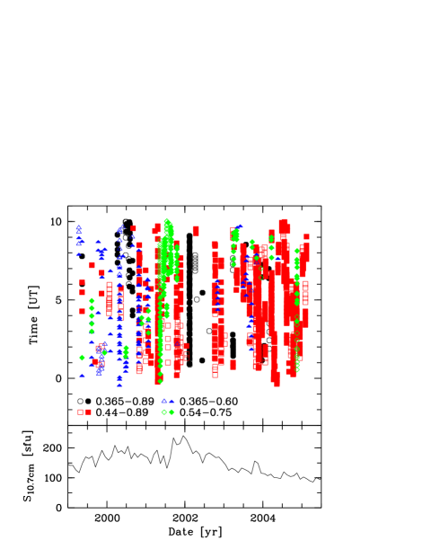
Figure 12: Date, time, and solar activity for the VLT FORS 1 observations of the Patat (PAT08 (2008)) spectroscopic data set. The solar activity is given by the solar radio flux measured at 10.7 cm in sfu. The FORS 1 spectra were taken with different instrument set-ups, which are indicated by different symbols and colours. The plot legend identifies the different set-ups by their covered wavelength ranges in $\mu$m. Open symbols indicate that the data were taken with the Moon above the horizon, whereas filled symbols refer to dark-time observations.

The airglow analysis (see Sects. 4.3 and 4.4) and the sky model verification (see Sect. 5) were carried out using a sample of 1186 FORS 1 long-slit sky spectra (see Fig. 12). The FORS 1 data were collected from the ESO archive and reduced by Patat (PAT08 (2008)). The spectra were taken with the low/intermediate resolution grisms 600B (12%), 600R (17%), and 300V, the latter with (57%) and without (14%) the order separation filter GG435. The set-ups cover the wavelength range from 0.365 to 0.89 $\mu$m. Wavelengths below 0.44 $\mu$m are the least covered, since only 600B and 300V spectra without GG435 can be used there. The FORS 1 spectra were taken between April 1999 and February 2005, i.e. observations during a phase of low solar activity are not part of the present data set (see Fig. 12). The mean and standard deviation of the Penticton-Ottawa solar radio flux at 10.7 cm (Covington COV69 (1969)) are 153 and 35 solar flux units (sfu = 0.01 MJy) respectively. The data set is also characterised by a mean zenith distance of $31\degr$. The corresponding standard deviation is only $13\degr$ and the maximum zenith distance is $67\degr$. The fraction of exposures with the Moon above the horizon amounts to 26%. 29 spectra were taken at sky positions with Moon distances below $30\degr$ (see Sect. 3.1). However, exposures affected by strong zodical light contribution are almost completely absent.

The FORS 1 night-sky spectra were not extinction corrected and the response curves for the flux calibration were derived by the Cerro Tololo standard extinction curve (Stone & Baldwin STO83 (1983); Baldwin & Stone BALD84 (1984)). We corrected all the spectra to the more recent and adequate Cerro Paranal extinction curve of Patat et al. (PAT11 (2011), see Sect. 2.1), assuming a mean airmass of 1.25 for the spectrophotometric standard stars. This procedure resulted in corrections of $+6$% at the blue end to $-1$% at the red end of the covered wavelength range.

4.3 Airglow lines

In the following, we treat airglow lines in detail. At first, the origin of the airglow line emission, the classification of lines, and a derivation of a line list for the sky model are discussed (Sect. 4.3.1). In the second part, we investigate the variability of airglow lines (Sect. 4.3.2).

4.3.1 Line classes and line list

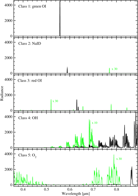
Figure 13: Variability classes for airglow emission lines. The following groups are defined: (1) green O I, (2) Na I D, (3) red O I, (4) OH, and (5) O₂. The weak lines (green curves) are scaled by a factor of 30 for Na I D, red O I, and O₂, and a factor of 10 for OH.

Table 2: Basic properties of the Paranal airglow line and continuum (0.543 $\mu$m) variability as derived from the Patat (PAT08 (2008)) spectral data set.

Property	Unit	[O I] 5577	Na I D	[O I] 6300,6364	OH(7,0)-(6,2)	O2(b-X)(0-1)	0.543 $\mu$m
$h_{\mathrm{\,layer}}$	km	97	92	270	87	94	90
$N_{\mathrm{spec}}$	–	1186	1046	1046	1046	839	874
$\langle I\rangle$	$\mathrm{phot\,s}^{-1}\,\mathrm{m}^{-2}\,\mathrm{arcsec}^{-2}$	3.6	0.81	3.5	60.	6.0	80.
		(1.6)	(0.48)	(3.4)	(19.)	(2.5)	(31.)
	R	190.	43.	190.	3200.	320.	4.3
		(90.)	(26.)	(180.)	(1000.)	(130.)	(1.6)
$m_{\mathrm{sun}}$	sfu-1	0.0087	0.0011	0.0068	0.0001	0.0063	0.0061
$P_{\mathrm{season,min}}$	–	1	1	1	5	5	1
$f_{\mathrm{season,min}}$	–	0.86	0.54	0.30	0.82	0.71	0.81
$P_{\mathrm{season,max}}$	–	3	3	3	6	3	3
$f_{\mathrm{season,max}}$	–	1.44	1.84	1.51	1.14	1.33	1.24

The most prominent optical airglow line is [O I] 5577 (see Fig. 13, panel 1). Its dominant component at an altitude of about 97 km is probably produced by the process described in Barth & Hildebrand (BAR61 (1961)). The crucial reactions are

$$\mathrm{O}+\mathrm{O}+\mathrm{M}\rightarrow\mathrm{O}^{*}_{2}+\mathrm{M},$$ (26)

$$\mathrm{O}^{*}_{2}+\mathrm{O}\rightarrow\mathrm{O}_{2}+\mathrm{O}(^{1}\mathrm{S}),$$ (27)

and

$$\mathrm{O}(^{1}\mathrm{S})\rightarrow\mathrm{O}(^{1}\mathrm{D})+557.7\,\mathrm{nm},$$ (28)

where M is an arbitrary reaction partner. The first reaction (Eq. 26) also plays an important role for the emission bands of molecular oxygen. In order to start the three body collision, oxygen molecules have to be split by hard UV photons:

$$\mathrm{O}_{2}+h\nu\rightarrow\mathrm{O}+\mathrm{O}.$$ (29)

This process mainly occurs during the day by solar UV radiation, which implies that the oxygen airglow intensity depends on the solar activity and observing time. The O$(^{1}{\rm D})$ state can lead to [O I] 6300 emission (see Fig. 13, panel 3). However, in the mesopause the deactivation of this metastable state is mostly caused by collisions. Hence, strong [O I] 6300 emission is restricted to the thermosphere at altitudes of about 270 km. In contrast to the mesosphere, the excitation there is caused by dissociative recombination (Bates BAT82 (1982)), i.e. it depends on the electron density:

$$\mathrm{O}^{+}_{2}+\mathrm{e}^{-}\rightarrow\mathrm{O}+\mathrm{O}(^{1}\mathrm{D}).$$ (30)

The ionised molecular oxygen is produced by the charge transfer reaction

$$\mathrm{O}^{+}+\mathrm{O}_{2}\rightarrow\mathrm{O}^{+}_{2}+\mathrm{O}.$$ (31)

The amount of ionised oxygen and free electrons depends on the solar radiation. The most striking features of the airglow are the Meinel OH bands (Meinel et al. MEI54 (1954)), which dominate at red optical wavelengths and beyond (see Fig. 13, panel 4). The fundamental and overtone rotational-vibrational transitions are mainly produced by the Bates-Nicolet (BAT50 (1950)) mechanism

$$\mathrm{O}_{3}+\mathrm{H}\rightarrow\mathrm{OH}^{*}+\mathrm{O}_{2}.$$ (32)

Most emission originates in a relatively thin layer at 87 km. Finally, the upper state of the prominent D lines of neutral sodium at 589.0 and 589.6 nm (see Fig. 13, panel 2), which originate in a thin layer at 92 km, is probably excited by

$$\mathrm{NaO}+\mathrm{O}\rightarrow\mathrm{Na}(^{2}\mathrm{P})+\mathrm{O}_{2}$$ (33)

(Chapman CHA39 (1939)). NaO appears to be provided by

$$\mathrm{Na}+\mathrm{O}_{3}\rightarrow\mathrm{NaO}+\mathrm{O}_{2}.$$ (34)

For studying airglow intensity and variability, we assigned the optical airglow lines to five classes, for which a similiar variability is reasonable or could be proved by a correlation analysis (see Patat PAT08 (2008)). These classes are (1) green O I, (2) Na I D, (3) red O I, (4) OH, and (5) O₂ (see Fig. 13). The first three classes correspond to atomic lines, the other two groups comprise molecular bands. The O I lines are divided into two classes. The green O I line at 557.7 nm mainly originates at altitudes slightly below 100 km, while the other significant O I lines (all being in the red wavelength range) tend to originate at altitudes greater than 200 km (see Khomich et al. KHO08 (2008)). Moreover, the kind of chemical reactions are also different, since the high altitude emissions are usually related to reactions involving ions (see above). Another small group consists of the sodium D lines and a weak K I line at 769.9 nm (see Fig. 13, panel 2). By far most of the airglow lines belong to the two classes of molecules which produce band structures by ro-vibrational transitions. The OH electronic ground state (X-X) bands with upper vibrational levels $v^{\prime}\leq 9$ cover the wavelength range longwards of about 0.5 $\mu$m with increasing band strength towards longer wavelengths. There are several electronic transitions with band systems for O₂ in the optical. Relatively weak bands of the Herzberg I (A-X) and Chamberlain (A’-a) systems originate at near-UV and blue wavelengths (see Cosby et al. COS06 (2006)). At wavelengths longwards of 0.6 $\mu$m, the atmospheric (b-X) band system produces several strong bands. However, those bands related to the vibrational $v=0$ level at the electronic ground state X are strongly absorbed in the lower atmosphere (see Sect. 4.1). Therefore, the only remaining strong band in the investigated wavelength range is O₂(b-X)(0-1) at about 864.5 nm (see Fig. 13, panel 5). Variability studies of O₂ have to rely on the results from this band.

For the identification of airglow lines and as an input line list for the sky model, we use the list of Cosby et al. (COS06 (2006)). It consists of 2805 entries with information on the line wavelengths, widths, fluxes, and line identities. It is based on the sky emission line atlas of Hanuschik (HAN03 (2003)), which was obtained from a total of 44 high-resolution ($R\sim 45000$) VLT UVES spectra. By combining different instrumental set-ups, the wavelength range from $0.314$ to $1.043$ $\mu$m could be covered. The accuracy of the wavelength calibration is better than 1 pm (cf. Sect. 4.1). The UVES spectra were flux calibrated by means of the Tüg (TUG77 (1977)) extinction curve. Since the use of a point-source extinction curve for the airglow leads to systematic errors (see Sect. 4.1) and the La Silla extinction curve was used for Cerro Paranal, we corrected the line extinction by means of the Patat et al. (PAT11 (2011)) extinction curve and the recipes given in Eqs. 24 and 25. At the lower wavelength limit, this caused an extreme correction factor of 0.37 and in the range of the O₂(b-X)(0-0) band a maximum factor of 4.5 due to the line molecular absorption correction (see Sect. 4.1). However, for the strongest 100 lines up to a wavelength of 0.92 $\mu$m, we only obtain a mean correction factor of 0.98. In a similar way as discussed in Sect. 4.2 for the Patat (PAT08 (2008)) data, we considered how a different extinction curve affects the response curves for flux calibration. Here, we obtain for the 100 brightest lines another correction of 0.97, which is representative of the factors for the entire wavelength range, which range from 0.95 to 1.00. Due to a gap at about 0.86 $\mu$m, the Cosby et al. (COS06 (2006)) line list misses a part of the important O₂(b-X)(0-1) band. There is an unpublished UVES 800U spectrum related to the study of Hanuschik (HAN03 (2003)) that covers the gap. We used this spectrum to measure the line intensities. Determined by a few overlapping lines, the resulting intensities were then scaled to those in the line list. For the line identification, we considered O₂ and OH line data from the HITRAN database (see Rothman et al. ROT09 (2009)). For the final line list for the sky model, the intensities of each variability class were scaled to match the mean value derived from the variability analysis (see below). Finally, the line wavelengths were converted from air to vacuum by

$$\lambda_{\mathrm{vac}}=n\,\lambda_{\mathrm{air}}.$$ (35)

The refractive index

$$n=1+10^{-8}\left(8342.13+\frac{2406030}{130-\sigma^{2}}+\frac{15997}{38.9-\sigma^{2}}\right),$$ (36)

where $\sigma=\lambda^{-1}$ and $\lambda$ is in $\mu$m (Edlén EDL66 (1966)). This formula is also used internally in the sky model code if an output in air wavelengths is required (see Table 1).

4.3.2 Line variability

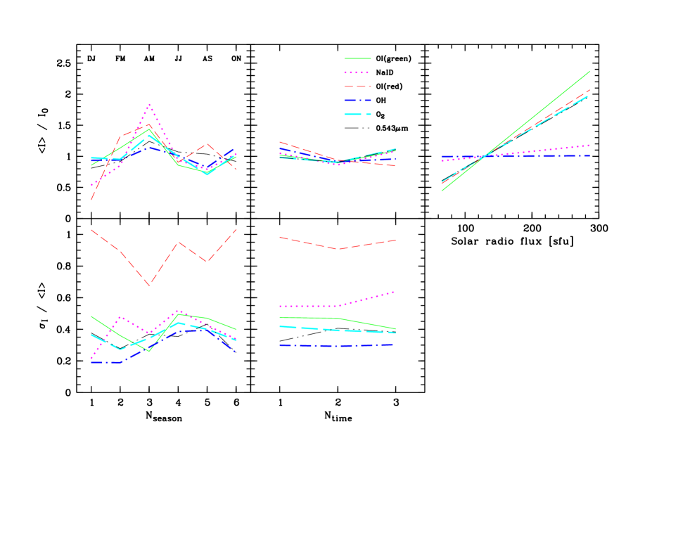
Figure 14: Variability correction for the five airglow line classes and the airglow continuum (analysed at 0.543 $\mu$m) of the sky model. Upper panels: The variability is shown as a function of the bimonthly period (1 = Dec/Jan, …, 6 = Oct/Nov), time bin (third of the night), and solar activity measured by the solar radio flux. Lower panels: For bimonthly period and time bin, the relative uncertainties of the variability correction are displayed.

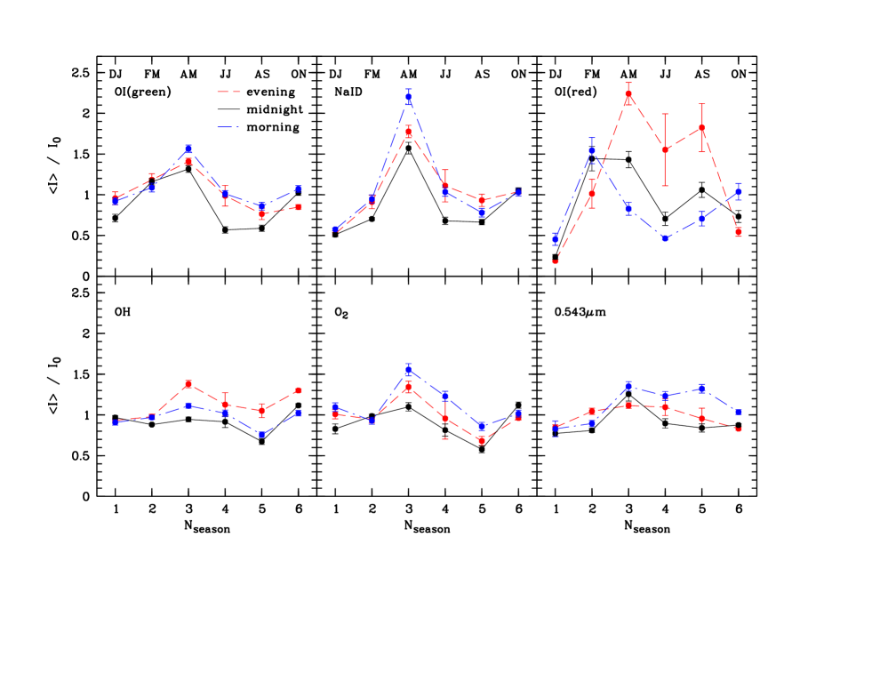
Figure 15: Variability correction factors and their errors depending on bimonthly period (1 = Dec/Jan, …, 6 = Oct/Nov) and night time (third of the night: evening, midnight, morning) for the five airglow line classes and the airglow continuum (analysed at 0.543 $\mu$m) of the sky model. Data points only differing in the bimonthly period are connected by lines.

In general, airglow lines show strong variability on time scales ranging from minutes to years. This behaviour can be explained by the solar activity cycle, seasonal changes in the temperature, pressure, and chemical composition of the emission layers, the day-night contrast, dynamical effects such as internal gravity waves and geomagnetic disturbances (see Khomich et al. KHO08 (2008)). In order to consider airglow variability in our sky model, we derived a semi-empirical model based on 1186 VLT FORS 1 sky spectra (Patat PAT08 (2008); see Sect. 4.2). The demands on an airglow variability model are twofold. First of all, it should include all major predictable variability properties. This excludes stochastic wave phenomena like gravity waves. Second, the derived parametrisation should be robust. For studying many variability triggers, about 1000 spectra is not statistically a high number. For this reason, only a few variables can be analysed. Since this neglection leads to higher uncertainties, an ideal set of parameters has to be found that provides statistically significant, predictable variations. For our airglow model, we studied the effect of solar activity, period of the year, and time of the night. The analysis was carried out for each of the five variability classes (see Fig. 13).

The first step for measuring the line and band fluxes was the subtraction of scattered moonlight, scattered starlight, and zodiacal light by using the recipes given in Sect. 3. The resulting spectra were then corrected for airglow continuum extinction as described in Sect. 4.1. For the flux measurements, continuum windows were defined. Their central wavelengths are listed in Table 3. The widths were 4 nm, except for 0.767 $\mu$m, where 0.3 nm was chosen to reduce the contamination by strong OH lines and the O₂(b-X)(0-0) band (see also Sects. 4.1 and  4.4). Then, the continuum fluxes were interpolated to obtain line and band intensities. The hydroxyl bands between 0.642 and 0.858 $\mu$m, i.e. OH(6-1) to OH(6-2), and the O₂(b-X)(0-1) band between 0.858 and 0.872 $\mu$m were measured automatically. In a second iteration, this procedure was improved by subtracting the obtained O₂ bands from the OH bands and vice versa before the intensity measurement. This way, the contamination by undesired lines can be minimised. Apart from the bands, the lines [O I] 5577, Na I D, [O I] 6300, and [O I] 6364 were analysed. The continuum fit is very critical for these lines, because of the narrow width of the features and the significant contamination by OH lines. For this reason, the line measurements were also manually performed for a subsample of 15 spectra for each instrumental set-up. The results were then used to derive intensity-dependent correction functions for the automatic procedure. Finally, the resulting band and line fluxes were corrected for the discrepancy between the molecular absorption of continuum and lines (see Sect. 4.1). These corrections were usually very small, since the strongest lines of each class do not overlap with significant telluric absorption.

A variability model can be efficiently determined by deriving a reference intensity and then applying multiplicative correction factors for each variability parameter (cf. Khomich et al. KHO08 (2008)). As a reference value for each variability class, we define the mean intensity at zenith for the five solar cycles 19 to 23, i.e. the years 1954 to 2007. The zenith intensity can be estimated by a correction for the van Rhijn effect (Eq. 21). The correction factors depend on the target zenith distance and the emission layer height (see Table 2). For describing the solar activity, we take the Penticton-Ottawa solar radio flux at 10.7 cm $S_{\mathrm{10.7\,cm}}$ (Covington COV69 (1969); see also Sect. 4.2). For the defined period, we derive a mean flux of 129 sfu. We can also derive a mean $S_{\mathrm{10.7\,cm}}$ for the spectroscopic sample. For this purpose, we obtained the monthly $S_{\mathrm{10.7\,cm}}$ averages corresponding to each spectrum. Due to the delayed response of the Earth’s atmosphere regarding solar activity of up to several weeks (see e.g. Patat PAT08 (2008)), monthly values are more suitable than diurnal ones. In the end, a mean $S_{\mathrm{10.7\,cm}}$ of 150 sfu could be derived for the entire FORS 1 data set. By performing a regression analysis for the relation between line intensity and $S_{\mathrm{10.7\,cm}}$ for each line class, we were able to obtain correction factors for a scaling of the lines to intensities typical of the reference solar radio flux. The resulting mean fluxes for the different classes were used to correct the fluxes in the reference line list (see Sect. 4.3.1). To derive the scaling factors, we integrated over all the listed lines in a class that were measured in the spectra. This required adding up the OH intensities of all bands from (6,1) to (6,2) and summing up the fluxes of the [O I] 6300 and [O I] 6364 lines, which have a fixed 3:1 intensity ratio. The extinction-corrected Cosby et al. (COS06 (2006)) intensities had to be corrected by factors between 0.43 for the red O I lines and 1.06 for Na I D lines to reach the intensities for the reference conditions. These reference intensities are given in Table 2. They are slightly lower than those in Patat (PAT08 (2008)) due to the lower mean solar radio flux.

The $S_{\mathrm{10.7\,cm}}$-dependent linear fits to the airglow intensities (see also Patat PAT08 (2008)) are also used to parametrise a correction of solar activity for our sky model. Even though the parametrisation is reasonable (cf. Khomich et al. KHO08 (2008)), there may be systematic deviations for monthly $S_{\mathrm{10.7\,cm}}$ beyond the data set limits of 95 and 228 sfu (see Sect. 4.2). With the dependence on solar radio flux removed, seasonal and nocturnal variations can be investigated. Since the intensity has a complex dependence on these parameters (see Khomich et al. KHO08 (2008)), we divided the data set into 6 seasonal and 3 night-time bins. In the same way as described in Sect. 2.1 for the transmission curves, the two-month periods start with the December/January combination. The night, as limited by the astronomical twilight, is always divided into three periods of equal length. This means that in winter the periods are longer than in summer. For the latitude of Cerro Paranal (see Sect. 1), the Dec/Jan night bins are about 30% shorter than the Jun/Jul bins. Due to the additional consideration of specific averages over the entire year and/or night, the total number of bins defined for the sky model is 28 (see also Table 1). Since the number of spectra in the individual bins differed by an order of magnitude, the average values over several bins could be biased. Therefore, all bins were filled with the same number of spectra by randomly adding spectra from the same bin, i.e. the data were cloned. This approach was also used for deriving the reference intensities. As a consequence, the mean solar radio flux of the data set changed from 153 (see Sect. 4.2) to 150 sfu. Finally, mean values and standard deviations were calculated for the individual and multiple bins using the original and bias-corrected data sets respectively. While the mean value provides an intensity correction factor for seasonal and/or night-time dependence, the standard deviation indicates the contribution of neglected variability components to the measured intensity. It also depends on the data quality, uncertainties in the analysis, and the accuracy of other sky model components. Therefore, the standard deviation of each bin should be an upper limit for the unmodelled airglow variability in the investigated data set.

The results of the airglow variability study are summarised in Table 2, and Figs. 14 and 15. The solar activity strongly influences the intensities of O I and O₂, where the slopes are 0.0063 to 0.0087 sfu^-1. On the other hand, weak or no significant correlations are present for sodium and hydroxyl. These findings are in qualitative agreement with the relations given in Khomich et al. (KHO08 (2008)), who provide 0.0025 to 0.0060 sfu^-1 for the first and about 0.0015 sfu^-1 for the second group from measurements at different observing sites (mainly in the Northern Hemisphere). The relatively low value of 0.0025 sfu^-1 for the green O I line compared to 0.0087 sfu^-1 from our model is not critical. A more precise latitude-dependent analysis of satellite-based data by Liu & Shepherd (LIU08 (2008)) resulted in 0.0065 sfu^-1 for the latitude range from $-20\degr$ to $-30\degr$. For $-30\degr$ to $-40\degr$ they even obtain the same slope as in our model. The discrepancies in the results from literature show that quantitative comparisons are difficult with different observing sites, observing periods, instruments, and analysis methods. Solar activity directly affects the Earth’s atmosphere by the amount of hard UV photons. The higher the photon energy, the more the production rate depends on solar activity (see Nicolet NIC89 (1989)). This relation appears to be important for O I and O₂ airglow emission, which depends on the dissociation or ionisation of molecular oxygen by hard UV photons (see Sect. 4.3.1).

Significant dependence on the bimonthly period is found for all line classes (see Fig. 14). Na I D and the red O I lines indicate the strongest variability with a maximum intensity ratio of 3.4 and 5.0 respectively, whereas OH shows the weakest dependence with a ratio of 1.4 (see Table 2). Except for OH, the maximum is reached in the autumn months April and May. For the atomic lines, the minimum arises in Dec/Jan, and for the molecular bands, it appears to be in Aug/Sep. The variations found reflect the semi-annual oscilliations of airglow intensity (cf. Patat PAT08 (2008)), which are characterised by two maxima and minima of different strength per year. Complex empirical relations based on long-term observations at many observing sites as given by Khomich et al. (KHO08 (2008)) can be used to estimate this intensity variation. However, since these relations depend on rough interpolations and extrapolations, they can only provide a coarse variability pattern for an arbitrary location on Earth. Nevertheless, these relations confirm the amplitude of the variations and the rough positions of the maxima and minima. For example, the peak-to-peak ratios for green O I, Na I D, and OH are 1.4, 3.8, and 1.3, which agrees well with the sky model values 1.7, 3.4, and 1.4 (see Table 2). Apart from the obvious change of the incident solar radiation, the seasonal variations are related to changes in the layer heights of the atmospheric constituents, changes in the temperature profiles, and the dynamics of the upper atmosphere in general.

Averaged over the year, the dynamical range of the night-time variations is in the order of 20 to 30%, which is distinctly smaller than the seasonal variations. Only the red O I lines show a clear decrease by a factor of 1.4 from the beginning to the end of the night. Usually, the diurnal variations are the largest in airglow intensity with possible amplitudes of several orders of magnitude (see Khomich et al. KHO08 (2008)). Since we exclude daytime and twilight conditions with direct solar radiation, the variability is much smaller. In addition, the use of only three bins can smooth out the intensity variations. However, an investigation with the unbinned data (see also Patat PAT08 (2008)) and results from photometric studies (Mattila et al. MAT96 (1996); Benn & Ellison BEN98 (1998); Patat PAT03 (2003)) confirm the absence of strong trends. Averaging over all bimonthly periods appears to cancel part of the variability. This is illustrated in Fig. 15, which shows the bimonthly dependence of the airglow intensity for each third of the night. At midnight, i.e. the maximum time distance to the twilight, the intensities of the mesopause lines tend to reach a minimum. However, the deviations from the intensities of the evening and morning bins appear to be a function of season. While in winter the differences reach a maximum, summer has the smallest differences. This behaviour can be explained by the night lengths at Cerro Paranal, which can vary by more than 30%. In summer, the average length of time from the closest twilight is significantly smaller than in winter. This dependence supports the common treatment of seasonal and night-time variations in the sky model.

The residual statistical variations of the airglow model, as depicted in Fig. 14, are mainly between 20 and 50% for the lines originating in the mesopause region. The smallest uncertainties are found for OH in summer, whereas the ionospheric O I lines indicate very strong unpredictable variations with an amplitude comparable to the intensity itself (see also Patat PAT08 (2008)). This behaviour is caused by the aurora-like intensity fluctuations from geomagnetic disturbances. This effect is particularly important for Cerro Paranal, because of its location close to one of the two active regions about $20\degr$ on either side of the geomagnetic equator (Roach & Gordon ROA73 (1973)).

4.4 Airglow continuum

The airglow continuum is the least understood emission component of the night sky. In the optical, the best-documented process is a chemiluminescent reaction of nitric oxide and atomic oxygen in the mesopause region as proposed by Krassovsky (KRA51 (1951)):

$$\mathrm{NO}+\mathrm{O}\rightarrow\mathrm{NO}_{2}+h\nu$$ (37)

$$\mathrm{NO}_{2}+\mathrm{O}\rightarrow\mathrm{NO}+\mathrm{O}_{2}.$$ (38)

This reaction appears to dominate the visual and is expected to have a broad maximum at about 0.6 $\mu$m (see Sternberg & Ingham STE72a (1972); von Savigny et al. SAV99 (1999); Khomich et al. KHO08 (2008)). Reactions of NO and ozone could be important for the airglow continuum at red to near-IR wavelengths (Clough & Thrush CLO67 (1967); Kenner & Ogryzlo KEN84 (1984)). In particular, the reaction

$$\mathrm{NO}+\mathrm{O}^{*}_{3}\rightarrow\mathrm{NO}^{*}_{2}+\mathrm{O}_{2}$$ (39)

is expected to significantly contribute to the optical by continuum emission with a broad maximum at about 0.85 $\mu$m (Kenner & Ogryzlo KEN84 (1984); Khomich et al. KHO08 (2008)). Finally, a pseudo continuum by molecular band emission produced by

$$\mathrm{Fe}+\mathrm{O}_{3}\rightarrow\mathrm{FeO}^{*}+\mathrm{O}_{2}$$ (40)

(West & Broida WES75 (1975)) could be an important component of the continuum between 0.55 and 0.65 $\mu$m (Jenniskens et al. JEN00 (2000); Evans et al. EVA10 (2010); Saran et al. SAR11 (2011)).

Table 3: Airglow/residual continuum and its intensity variation relative to the reference wavelength 0.543 $\mu$m.

$\lambda$ [$\mu$m]	$\langle I\rangle/I_{0}$	$\sigma_{I}/I_{0}$	$\sigma_{I}/\langle I\rangle$
0.369	0.92	0.13	0.14
0.387	0.65	0.11	0.17
0.420	0.69	0.10	0.15
0.450	0.70	0.11	0.15
0.480	0.79	0.11	0.14
0.510	0.79	0.09	0.12
0.543	1.00	0.00	0.00
0.575	1.41	0.25	0.18
0.608	1.40	0.29	0.20
0.642	1.18	0.19	0.16
0.675	1.14	0.13	0.12
0.720	1.32	0.21	0.16
0.767	1.64	0.46	0.28
0.820	2.57	0.67	0.26
0.858	3.56	1.06	0.30
0.872	3.76	1.12	0.30

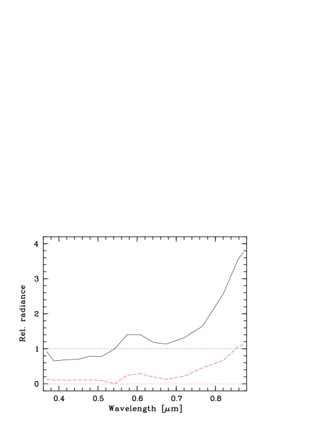
Figure 16: Airglow/residual continuum (solid line) and its variability (dashed line) relative to the reference wavelength $0.543$ $\mu$m.

The airglow continuum was analysed in a similar way as the airglow emission lines. As reported in Sect. 4.3.2, the derivation of line intensities already required the measurement of airglow continuum fluxes in suitable windows (see Table 3). These results were refined by subtracting possible contributions from airglow lines by applying the line emission model as described in Sect. 4.3. For the variability analysis, the Patat (PAT08 (2008)) data set (see Sect. 4.2) was restricted to the 874 FORS 1 spectra, where the Moon was below the horizon. This avoids large errors in the continuum flux from the subtraction of a bright and uncertain component (see Sect. 3.1). Even though the absolute uncertainties of the other components are significantly smaller, the derived continuum is a residual continuum. It is affected by uncertainties in zodical light brightness, scattered starlight, airglow line emission, molecular absorption, possible unconsidered minor components, scattered light from dispersive elements, and flux calibration of the spectra. While the other sky model components should cause an uncertainty in the order of a few per cent only (for 0.767 $\mu$m this could be somewhat higher, see Sect. 4.3.2), the uncertainty in the flux calibration could be significantly more. Since theoretical components are subtracted from the observed spectra to obtain the airglow continuum, errors in the flux calibration have a larger effect on the resulting continuum than on the total spectra. For example, for a 50% contribution of the continuum to the total flux, a flux error of 10% would convert into a continuum error of 20%.

For the subsequent analysis, we defined a reference continuum wavelength. Due to its availability in all spectroscopic modes and the absence of contaminating emission lines, we selected 0.543 $\mu$m. In the following, we studied the continuum relative to this wavelength, i.e. the mean continuum was derived by scaling the fluxes to the reference solar radio flux of 129 sfu (see Sect. 4.3.2) by using only the linear regression results and binning corrections derived for 0.543 $\mu$m. This approach means that a fixed shape of the continuum is assumed. This simplified variability model can be more easily used in the sky model. As shown by the last column of Table 3, there are relatively low variations of the continuum flux relative to the reference flux for the investigated data set. For most wavelengths, the standard deviation divided by the mean flux $\sigma_{I}/\langle I\rangle$ is lower than 20% and only reaches 30% at the reddest wavelengths. In view of all the uncertainties discussed above, which also contribute to these numbers, the assumption of a fixed continuum slope is sufficient for an application for the ETC sky background model. This assumption is also supported by the high correlation factors for different continuum windows measured by Patat (PAT08 (2008)). It should be noted that the number of available spectra decreases towards the margins in the analysed spectral range due to the different instrumental set-ups (see Sect. 4.2). In particular, wavelengths shortwards of 0.44 $\mu$m have only 239 spectra, i.e. 27% of the sample used for 0.543 $\mu$m. The change in the sample size as well as different systematic errors in the response curves for the different set-ups cause systematic uncertainties in the airglow continuum shape. By comparing the mean fluxes in overlapping wavelength regions of the different set-ups, we estimate an uncertainty in the order of 10%.

We obtained a mean airglow continuum for Cerro Paranal with an intensity of about 4.3 $\mathrm{R}\,\mathrm{nm}^{-1}$ at 0.543 $\mu$m (for R[ayleigh] units see Table 2). The corresponding variability is 1.6 $\mathrm{R}\,\mathrm{nm}^{-1}$. Considering the latitude of Cerro Paranal, this result is in good agreement with observations that suggest an increase of the airglow continuum from $1-2\,\mathrm{R}\,\mathrm{nm}^{-1}$ at the equator to $10-20\,\mathrm{R}\,\mathrm{nm}^{-1}$ in the polar region for similar wavelengths (see Davis & Smith DAV65 (1965); Khomich et al. KHO08 (2008)). As illustrated in Fig. 16 and listed in Table 3, the mean airglow continuum is characterised by a broad bump at about 0.6 $\mu$m and an increase in intensity towards longer wavelengths with a steep slope at about 0.8 $\mu$m. The continuum in the bump region appears to be mainly produced by two processes: a relatively smooth $\mathrm{NO}+\mathrm{O}$ continuum (see Eq. 37) and a more structured $\mathrm{Fe}+\mathrm{O}_{3}$ continuum (see Eq. 40) showing a peak at about 0.6 $\mu$m (see Evans et al. EVA10 (2010)). If the bump, which indicates a width of about 0.1 $\mu$m, could be completely explained by the iron oxide reaction, this component would contribute up to $1/3$ of the mean airglow continuum flux (see also Sect. 5.1). Towards longer wavelengths, it is not clear whether the observed increase in intensity is mainly caused by relatively narrow peaks or a smooth increase (see Sternberg & Ingham STE72a (1972); Sobolev SOB78 (1978); Content CON96 (1996)). Up to 0.872 $\mu$m, our measurements suggest a monotonic increase beyond the 0.6 $\mu$m bump. Intensities of about 15 $\mathrm{R}\,\mathrm{nm}^{-1}$, as found by Sternberg & Ingham (STE72a (1972)) and Sobolev (SOB78 (1978)) at wavelengths longwards of $0.8$ $\mu$m, are in good agreement with our mean spectrum, with the same intensity at about $0.86$ $\mu$m. Also, the intensities of Sternberg & Ingham (STE72a (1972)) and of the sky model mean airglow continuum are very similar at our reference wavelength in the $V$ band. A possible production meachanism for the strong increase at about 0.8 $\mu$m could be a reaction of nitric oxide with excited ozone (see Eq. 39), for which a peak wavelength of about 0.85 $\mu$m is expected (see Kenner & Ogryzlo KEN84 (1984); Khomich et al. KHO08 (2008)). Then, the strong intensity increase would be the blue wing of the bump from this reaction. The slope does tend to decrease where the peak is predicted, and the continuum variations there relative to 0.543 $\mu$m (see $\sigma_{I}/\langle I\rangle$ in Table 3) are the highest. This could be another argument for different chemical processes producing the emissions at 0.55 and 0.85 $\mu$m.

As in the case of the airglow lines, the intensity of the sky model airglow continuum measured at $0.543$ $\mu$m depends on zenith distance, solar radio flux, period of the year, and period of the night. The results are shown in Table 2, and Figs. 14 and 15. The dependence of the continuum emission on solar radio flux is significant and comparable to O I (green and red) and O₂. Since OH does not indicate a significant dependence on $S_{\mathrm{10.7\,cm}}$, the continuum must be the main source for the dependence of the broad-band fluxes on solar activity (cf. Walker WAL88 (1988); Patat PAT03 (2003), PAT08 (2008)). Concerning the seasonal and nocturnal variations, the continuum at $0.543$ $\mu$m tends to show the best agreement with OH, i.e. the variability of these parameters is relatively low. The maximum ratio of the bimonthly mean intensities is only about 1.5 (cf. Patat PAT08 (2008)).

5 Discussion

After describing all the optical model components in the previous sections, we now discuss the quality of the sky model as a whole by comparing it to the Patat (PAT08 (2008)) data set of sky spectra and results found in the literature. First, sky model spectra and observed spectra are compared (Sect. 5.1). Second, a systematic quality evaluation by means of broad-band photometry of our model with data, and a comparison to the night-sky brightnesses from the literature are discussed in Sect. 5.2. Finally, we evaluate the improvements achieved by our sky model compared to the current ESO ETC sky background model in the optical (Sect. 5.3).

5.1 Comparison of spectra

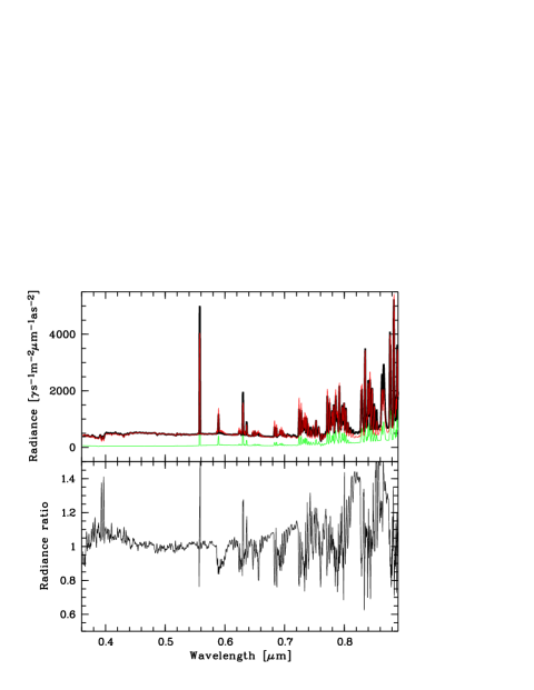
Figure 17: Comparison of the sky model (upper panel: thick black line) and an observed FORS 1 300V spectrum (thin red line) with moderate lunar contribution (see Table 1). The uncertainty of the sky model due to airglow variability is also shown (green). The lower panel exhibits the ratio of the sky model and the observed spectrum.

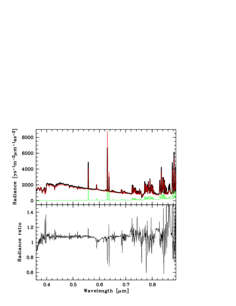
Figure 18: Comparison of the sky model and an observed FORS 1 300V spectrum with strong lunar contribution. For an explanation of the different curves, see Fig. 17.

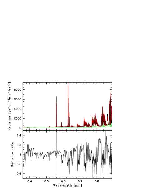
Figure 19: Comparison of the sky model and an observed FORS 1 300V spectrum without lunar contribution, but strong airglow emission lines. For an explanation of the different curves, see Fig. 17.

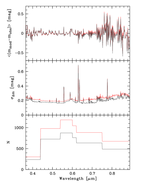
Figure 20: Deviations between the sky model and the observed FORS 1 spectra in magnitudes. The mean magnitude difference (upper panel), the standard deviation (middle panel), and the wavelength-dependent number of considered spectra (lower panel) are shown for 1 nm bins. Results for the full spectroscopic data set (red) and for spectra with the Moon below the horizon (black) are displayed.

In order to evaluate the quality of our sky model, spectra were computed for the different instrumental set-ups and observing conditions of the Patat (PAT08 (2008)) data set (see Sect. 4.2). A detailed description of the sky model input parameters can be found in Table 1. Before the full data set is discussed, we show a few typical sky model spectra in comparison with the corresponding observed spectra (Figs. 17 to 19).

In the optical, the relevant sky model components are scattered moonlight, scattered starlight, zodiacal light, and airglow lines and continuum of the upper atmosphere (see Fig. 1). Figure 17 compares a typical FORS 1 spectrum exhibiting moderate Moon contribution to the corresponding sky model. This and the FORS 1 spectra of the other figures were taken with the 300V grism without order separation filter. This set-up provides the maximum wavelength range. Due to the missing order separation filter, there can be a slight ($\la 10\%$) contamination by the second order spectrum at red wavelengths. However, this does not affect the quality of the sky model (see Sect. 5.2), because of the small number of spectra used in the analysis. Figure 17 demonstrates that the different sky model components agree reasonably well with the observed spectrum. Apart from the reddest part of the spectrum, deviations of 10 to 20% are typical. The best agreement is found for the continuum in the visual. Residuals of strong sky lines in the ratio plot in the lower panel appear more prominent than the real values due to slight differences in the instrumental profiles of the model and the observed spectrum.

Figure 18 shows the effect of a strong Moon contribution on the sky model. Scattered moonlight dominates the continuum at all wavelengths in the displayed range. At blue wavelengths, the example spectrum reaches up to 2000 $\mathrm{photons\,\,s}^{-1}\,\mathrm{m}^{-2}\,\mu\mathrm{m}^{-1}\,\mathrm{arcsec}^{-2}$. In contrast, during moonless nights the values are about one order of magnitude lower (see Fig. 19). Even though the deviations between the sky model and the observed spectrum are not larger than 10% for most of the continuum, there is a systematic trend. For a wide wavelength range, the sky model appears to be too bright by a relatively constant factor. Apart from deviations of the Moon illuminance from the model in Eq. 15, this discrepancy could be explained by uncertainties in the Mie scattering model, since this changes slowly with wavelength (see Fig. 2). Moreover, the angular distance between Moon and target $\rho=44\degr$ is small enough for significant Mie scattering. Similar trends with positive as well as negative deviations are observed in other cases of high lunar sky brightness. As already mentioned in Sect. 3.1, the amplitude of the differences tends to increase for decreasing $\rho$. Nevertheless, the uncertainties of the extended Krisciunas & Schaefer (KRI91 (1991)) model are usually not critical for spectra with low to moderate lunar contribution, as it is illustrated in Fig. 17.

A spectrum without scattered moonlight is shown in Fig. 19. In this case, the contiuum is mainly a combination of zodiacal light and airglow continuum. Scattered starlight only adds a few per cent to the total continuum emission. In the $B$ and $V$ bands, the continuum of dark-time exposures is usually well reproduced by the sky model. At longer wavelengths, the uncertainties increase from the significant (and partly unpredictable) variability of the airglow continuum and the simplifying assumption of a fixed continuum shape (see Sect. 4.4). The three spectra shown indicate deviations between 20 to 40% at about 0.82 $\mu$m. By chance, the sky model is brighter than the observed spectrum in all cases. Airglow emission lines can vary significantly, depending on the line class, observing direction, solar activity, season, and time of night. Even though there is always a stochastic component, which cannot be modelled, the sky model accounts for such variations quite well. The uncertainty of the line modelling for the spectra shown is in the order of 20%. The spectra in Figs. 17 and 19 were taken at the same solar radio flux (205 sfu) and in the last third of the night, i.e. the conspicuous differences between both spectra can mainly be explained by seasonal variations. This is confirmed by the fact that the sky model can roughly follow the striking changes in the intensities of the red O I lines (cf. FM and JJ periods for red O I morning intensities in Fig. 15).

For a more systematic comparison between the model and the data, we computed the mean and standard deviations for the entire sample and a subset with the Moon above the horizon. The number of spectra involved depends on the wavelength and does not exceed 1186 and 874 respectively. The results are displayed in Fig. 20 in magnitudes. For both samples, the systematic model deviations (upper panel) are close to zero. This is very satisfying, but not unexpected. The airglow line and continuum components were derived based on the FORS 1 spectra, which are also used in the comparison. The lack of clear spectral features in the upper panel of Fig. 20 suggests that the model quality is similar at all wavelengths. As already discussed in Sect. 4.4, the real accuracy of the model also depends on the quality of the flux calibration of the Patat (PAT08 (2008)) data. The uncertainties can be in the order of 10%, and so this appears to be the main source of systematic errors in the model intensities.

The standard deviation of the magnitude differences between the model and observed data $\sigma_{\Delta m}$, shown in the middle panel of Fig. 20, indicates an interesting wavelength dependence. For the dark-time sample, the continuum uncertainty ranges between 0.16 and 0.24 mag. Including observations with scattered moonlight increases these values to 0.19 and 0.28 mag. The additional variation is mainly caused by a few spectra with large uncertainties in the Mie scattering of moonlight (see above). These results suggest that the relative strong continuum deviations at 0.82 $\mu$m, as in Figs. 17 and 19, are relatively high compared to the entire sample. The spectrum of $\sigma_{\Delta m}$ shows a relatively broad feature at about 0.6 $\mu$m, which is reminiscent of the shape of the FeO pseudo continuum (see Jennikens et al. JEN00 (2000); Evans et al. EVA10 (2010); Saran et al. SAR11 (2011)). This result supports the assumption that the airglow continuum bump at 0.6 $\mu$m (see Fig. 16) is mainly produced by iron oxide (see Sect. 4.4) and varies differently than the underlying NO₂ continuum, for which the intensitiy changes at 0.543 $\mu$m are considered by the sky model. Fig. 20 indicates a FeO-related variability of about 15%. Since the mean bump contributes about 20% of the total flux at 0.6 $\mu$m, the variation is almost comparable to it. These strong variations are in agreement with previous results (see Evans et al. EVA10 (2010); Saran et al. SAR11 (2011)). A minor source of continuum variability at 0.6 $\mu$m is the Chappuis ozone bands (see Fig. 2), which indicate a variation of 0.02 mag airmass^-1 (see Patat et al. PAT11 (2011)). The middle panel of Fig. 20 does not exhibit strong signatures of OH bands (see Fig. 13, panel 4). The bands are clearly detectable only in the range of low continuum uncertainty. Consequently, the quality of the OH modelling is comparable or even better than the continuum modelling. This is particularly important for the quality of the full sky model at long wavelengths, where OH emission dominates the spectra. The sky model is less able to model atomic lines, as shown in Fig. 20. The maximum variability of 0.7 mag is found at [O I] 6300. In addition, other lines of the thermospheric ionosphere, which are usually difficult to recognise (see Fig. 13, panel 3), significantly contribute to $\sigma_{\Delta m}$. For example, N I at 520 nm and O I at 616, 656, and 777 nm are clearly detectable. This confirms the conclusion of Sect. 4.3.2, stating that the intensities of ionospheric lines are difficult to predict due to their sensitivity to geomagnetic disturbances (see Roach & Gordon ROA73 (1973)).

5.2 Comparison of photometry

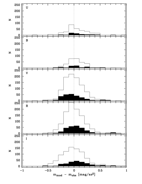
Figure 21: Histograms for the deviations of the sky model from the FORS 1 data in mag for the filters $U$, $B$, $V$, $R$, and $I$. The filled histograms show only data with the Moon above the horizon.

Table 4: Comparison of the sky model and the Walker (WAL87 (1987)) magnitudes with the Patat (PAT08 (2008)) FORS 1 data.

Filter	All						No Moon
	$N$	$\langle\Delta m\rangle$	$\sigma_{\Delta m}$	$\sigma_{\rm obs}$	$\langle\Delta m_{\mathrm{w}}\rangle$	$\sigma_{\Delta m,\mathrm{w}}$	$N$	$\langle\Delta m\rangle$	$\sigma_{\Delta m}$	$\sigma_{\rm obs}$	$\langle\Delta m_{\mathrm{w}}\rangle$	$\sigma_{\Delta m,\mathrm{w}}$
$U$	303	$+0.053$	0.230	0.521	$-0.113$	0.725	239	$+0.042$	0.213	0.214	$-0.059$	0.703
$B$	303	$+0.046$	0.205	0.561	$+0.269$	0.430	239	$+0.048$	0.174	0.182	$+0.196$	0.407
$V$	979	$+0.000$	0.192	0.563	$+0.356$	0.409	727	$+0.006$	0.175	0.255	$+0.244$	0.322
$R$	1046	$+0.009$	0.199	0.447	$+0.169$	0.365	762	$-0.009$	0.177	0.260	$+0.083$	0.287
$I$	839	$-0.003$	0.238	0.365	$+0.413$	0.326	615	$-0.040$	0.208	0.287	$+0.365$	0.294

Table 5: Typical sky model and literature night-sky brightnesses in mag arcsec^-2 for zenith, no Moon, faint zodiacal light, and different solar radio fluxes.

Source	Site	$S_{\mathrm{10.7\,cm}}$	$U$	$B$	$V$	$R$	$I$
Benn & Ellison (BEN98 (1998))	La Palma	80	22.0	22.7	21.9	21.0	20.0
Walker (WAL87 (1987))	Cerro Tololo	90	22.0	22.7	21.8	20.9	19.9
Krisciunas et al. (KRI07 (2007))	Cerro Tololo	130	22.1	22.8	21.8	21.2	19.9
Mattila et al. (MAT96 (1996))	La Silla	150		22.8	21.7	20.8	19.5
Patat (PAT08 (2008))	Cerro Paranal	160	22.4	22.7	21.7	20.9	19.7
Patat (PAT03 (2003))	Cerro Paranal	180	22.3	22.6	21.6	20.9	19.7
Sky model	Cerro Paranal	90	22.3	22.9	22.0	21.2	19.8
		130	22.1	22.8	21.8	21.0	19.7
		180	21.9	22.6	21.6	20.9	19.6

To perform a more quantitative comparison of our sky model and observed data, and for an easier comparison to other studies, we derived magnitudes from broad-band filter fluxes. Specifically, we used the standard photometric system consisting of $U$, $B$, $V$, $R$, and $I$ (see Bessell BES90 (1990)). For the Patat (PAT08 (2008)) data and their corresponding sky models, only a grism-dependent subset of filters can be taken. The spectrum needs to cover $\ga 90$% of the filter curve. An exception is the $U$ filter, which extends below $0.365$ $\mu$m, the lower wavelength limit of the bluest spectral set-up (see Sect. 4.2). Therefore, the results for this filter are questionable.

Figure 21 and Table 4 show the results of the computations for the full sample of FORS 1 spectra and a subsample with the Moon below the horizon (cf. Sect. 5.1). Only a small fraction ($\sim 1/4$) of the spectra contribute to the mean values and standard deviations of the $U$ and $B$ filters. Most spectra cover the range of the $V$, $R$, and $I$ filters. For both samples and all filters, the mean magnitude differences are small ($\la 0.05$ mag). Even though the sky model tends to be slightly fainter at the blue end and slightly brighter at the red end, there are no serious systematic deviations from the observed spectra (cf. Sect. 5.1). The standard deviations $\sigma_{\Delta m}$ are relatively similar for the different filters. For the full sample, they range from 0.19 mag for the $V$-band to 0.24 mag for the $I$ band. Consequently, the accuracy of the sky model is in the order of about 20%. These values can be compared to the magnitude variations in the measured data $\sigma_{\rm obs}$, which correspond to $\sigma_{\Delta m}$ for an optimum sky model of time-invariant flux. For the full sample, the deviations are distinctly larger. They range from 0.37 to 0.56 mag. These large deviations are mainly due to the observations with a strong moonlight contribution (see Sect. 3.1). For dark-time conditions, $\langle\Delta m\rangle$ ranges from 0.17 mag for $B$ to 0.21 mag for $U$, and $\sigma_{\Delta m}$ indicates differences between 0.18 mag for $B$ and 0.29 mag for $I$. In particular, for the bands $V$ to $I$, a time-invariant sky model would be significantly worse than our sky model (see also Sect. 5.3). This shows the improvements from a variable zodiacal light, airglow lines, and airglow continuum model.

Finally, we compare the sky model to literature data. Magnitudes in the five broad-band filters $U$ to $I$ were calculated using standardised observing conditions. Specifically, zenith, New Moon, ecliptic pole, annual average, and mean solar activity, i.e. 130 sfu (see Sect. 4.3.2), were assumed. The resulting magnitudes are provided in Table 5. For a better comparison with published data, the table also contains sky model results for 90 and 180 sfu. The reference data in Table 5 originate from Mattila et al. (MAT96 (1996)) for La Silla, Walker (WAL87 (1987)) and Krisciunas et al. (KRI07 (2007)) for Cerro Tololo, Benn & Ellison (BEN98 (1998)) for La Palma, and Patat (PAT03 (2003), PAT08 (2008)) for Cerro Paranal. In general, there is a good agreement between the sky model and observed sky brightnesses. By comparing magnitudes with similar average solar radio fluxes, we find typical deviations in the order of 0.1 mag. An exception is the $U$ filter with typical differences of about 0.3 mag, which could be explained by the lower quality of the sky model at near-UV wavelengths due to the lack of data (see Sect. 4.2). Also, it is not clear to what extent components like zodiacal light or scattered starlight, which significantly affect short wavelengths, contribute to the observed data. The corresponding intensities can differ from those of the sky model for the assumed ideal conditions. The published photometry appears to confirm the lack of reproducibility of $U$-band magnitudes. Unexpectedly, the sky brightness seems to increase with decreasing solar activity. It should be noted that photometric samples are often too small to cover all of the airglow variability, which causes additional uncertainties. For the airglow continuum, which is a major contribution to the night-sky brightness in the optical, the intensity significantly depends on the geographic latitude (see Davis & Smith DAV65 (1965)). In summary, we can assume that our sky model calculates reliable night-sky brightnesses, at least for the levels of solar activity that could be analysed.

A comparison of the sky model with other studies can also be enlightening in terms of the night-sky variability, particularly the striking dependence of the sky brightness on solar activity (Walker WAL88 (1988); Mattila et al. MAT96 (1996); Krisciunas KRI97 (1997); Patat PAT03 (2003), PAT08 (2008)). For the range of photometric fluxes in $UVI$ under dark-time conditions at zenith, Patat (PAT08 (2008)) found 0.9, 1.3, and 1.7 mag. For the same filters, he estimated a flux increase of 0.6, 0.3, and 0.2 mag for a change in the solar radio flux from 80 to 240 sfu. In contrast, Walker (WAL88 (1988)) gives $\Delta B\approx 0.8$ mag and $\Delta V\approx 1.0$ mag for a similar solar activity change. About $0.5$ mag are reported by Mattila et al. (MAT96 (1996)) for blue wavelengths and by Krisciunas et al. (KRI97 (1997)) for the $V$ band. For a typical brightness of the zodiacal light of 1.7 times the intensity at the ecliptic pole and the same range of solar radio fluxes as used by Patat (PAT08 (2008)), the sky model gives 0.7, 0.5, 0.6, 0.6, and 0.3 mag for the $UBVRI$ filters. These values are consistent with the results from the other studies. The significant discrepancy of 0.3 mag to the Patat (PAT08 (2008)) result for the $V$ filter might be explained by the relative small sample of only 148 images and the general difficulties in separating the different sky radiation components by means of photometric data. For $B$ to $R$, the solar activity appears to be responsible for about half the night-sky variability. Since the zodiacal light variations cause a $1\,\sigma$ uncertainty of about 0.1 mag, as estimated from the FORS 1 data set, seasonal, nocturnal, and unpredictable short-term airglow variations should generate most of the remaining variability in $V$ and the adjacent bands.

5.3 Comparison to current ETC sky model

The main motivation for this study is to achieve a significant improvement over the current ESO ETC for a more efficient use of the VLT time. As discussed in Sect. 1, the current sky emission model for optical instruments consists of the Moon phase dependent, photometric sky brightness table of Walker (WAL87 (1987)) and an instrument-specific template spectrum scaled to the flux in the photometric filter closest to the centre of a given spectral setting. It does not consider any change in the relative contributions of the different sky emission components, which can be quite strong as discussed in the previous sections. Thus, we can expect that the model continuum level significantly deviates from the true one, even if the corresponding filter flux is correct. Our new sky model with variable model components is an important improvement.

For a more quantitative comparison of the current and our new sky model, we derived the Walker (WAL87 (1987)) magnitudes for the observing conditions of the Patat (PAT08 (2008)) FORS 1 data set (see Sect. 4.2). The resulting $U$ to $I$ magnitudes can be compared to the measured ones to analyse the quality of the two models (see also Sect. 5.2). Table 4 exhibits the mean deviation of the Walker model $\langle\Delta m_{\mathrm{w}}\rangle$ and the standard deviation of the difference $\sigma_{\Delta m,\mathrm{w}}$ for the full and the dark-time sample. Since the Walker magnitudes depend on the Moon phase, one can expect that the model based on his data set would have a lower scatter than an optimum time-invariant model given by $\sigma_{\rm obs}$. Except for the $U$ band, which is difficult to compare (see Sect. 5.2), this is true. For the full data set, the standard deviations are lower by 0.04 ($I$) to 0.15 mag ($V$). However, this improvement is small compared to the corresponding results for our sky model. For the $B$ and $V$ bands $\sigma_{\Delta m,\mathrm{w}}$ is more than twice as large as $\sigma_{\Delta m}$. Moreover, there are significant systematic mean deviations of 0.1 to 0.4 mag. For our sky model, the maximum value is 0.05 mag. Even though this benefits from the use of the same data for the derivation of the airglow line and continuum model, the offset with the Walker model is striking. It can be explained by the fact that the Moon phase is the only variable parameter. Therefore, the systematic changes of other parameters can cause significant magnitude offsets. For example, the fainter magnitudes of the Walker model can partly be explained by the very low solar activity (about 90 sfu), whereas the Patat (PAT08 (2008)) data set has a mean solar radio flux of 153 sfu.

The dark-time data provided by Table 4 show a decrease of $\sigma_{\Delta m,\mathrm{w}}$ by 0.02 ($B$) to 0.08 mag ($R$) compared to the values for the full sample. Excluding the $U$ band, the typical scatter of the Walker model is about 0.3 mag. This is worse than the results for our sky model and even a time-invariant model. For the $B$ band, the difference is more than 0.2 mag. For the $I$ band, the situation is better, since the Walker model almost reaches the standard deviation of the time-invariant model. Nevertheless, $\sigma_{\Delta m}$ of our sky model is still about 0.1 mag lower. The unsatisfactory performance of the Walker model is caused by the unconsidered, varying amount of scattered moonlight during a Moon phase. Even for phases close to Full Moon, dark-time observations are possible. For this reason, the scatter of the Walker model is larger than for a time-invariant model. The difference depends on the average contribution of scattered moonlight to the sky brightness, which is higher at shorter wavelengths. This effect causes an overestimation of the sky brightness for dark-time observations, which is indicated by a comparison of $\langle\Delta m_{\mathrm{w}}\rangle$ for the full and dark-time samples.

In summary, we can state that our sky model performs better than the current ESO ETC sky model for the optical by about several tenths of a magnitude. The quality difference should be even higher for a single wavelength instead of a broad-band filter. Even if the input parameters of our new sky model (see Table 1) could not optimally be constrained in the planning phase, due to uncertainties in the scheduling of the observations, there would be a significant improvement for the prediction of the signal-to-noise ratio for astronomical observations. This justifies the effort in developing an advanced sky model.

6 Summary and outlook

In this paper, we presented a sky model for the ESO observing site at Cerro Paranal to help predict the effects of the Earth’s atmosphere on astronomical observations in the optical. This sky model includes atmospheric extinction, scattered moonlight, scattered starlight, zodiacal light, and airglow emission lines and continuum.

• The atmospheric extinction is characterised by three components: Rayleigh scattering, aerosol extinction, and molecular absorption. For the former, we use the formula given by Liou (LIO02 (2002)). The aerosol extinction is based on the parametrisation of Patat et al. (PAT11 (2011)) for Cerro Paranal. The molecular absorption is calculated by the radiative transfer code LBLRTM for atmospheric profiles optimised for the observing site.

• Scattered moonlight is derived from the Krisciunas & Schaefer (KRI91 (1991)) model for the $V$ band, which is extrapolated for the entire optical range using the solar spectrum and the Cerro Paranal extinction curve.

• For scattered starlight, a mean spectrum was derived by 3D single scattering calculations with multiple scattering corrections, using the Toller (TOL81 (1981)) integrated starlight distribution and the mean spectrum of Mattila (MAT80 (1980)).

• The zodiacal light is computed based on the model given by Leinert et al. (LEI98 (1998)). Scattering of the zodiacal light in the Earth’s atmosphere is also treated with 3D scattering calculations.

• Airglow emission lines and continuum are highly variable. We used a set of 1186 VLT FORS 1 sky spectra (Patat PAT08 (2008)) taken during a wide range of conditions to parametrise a model for five line and one continuum variability classes. The line wavelengths and intensities are based on the atlas of Hanuschik (HAN03 (2003)), improved by the results of the variability analysis. For the airglow scattering, 3D calculations were used as well.

After summing over all the components, we then compared the sky model with observed sky spectra. We found that our model is accurate to about 20%. This could only be achieved by having variable model components, especially the airglow model, which is a significant improvement over previous models. The mean sky brightnesses and variations derived from our model are in good agreement with results from other photometric studies. Compared to the current ETC sky model, the accuracy is increased by several tenths of a magnitude.

There are new results from this sky model study:

• We found scattering scaling relations for the extended radiation sources zodiacal light and airglow. These are new simple relations to derive effective extinction curves. The corresponding correction factors for the point-source extinction curve only depend on the unextinguished line-of-sight intensity of the radiation source.

• We characterised the variability of the airglow line and continuum emission at Cerro Paranal based on several input parameters, such as period of the year, time of night, and solar radio flux.

• We derived long-term mean airglow line and continuum intensities. For the latter, we benefit from the modelling of the intensity of the other sky model components. We could determine the shape of the optical airglow continuum with high accuracy. For the controversial wavelength range longwards of 0.7 $\mu$m, we find a smooth intensity increase. This could be produced by chemical reactions different from those dominating the shorter wavelengths. The well-known peak at 0.6 $\mu$m was identified as strongly varying.

The model presented in this paper is aimed at the ETC for optical VLT imagers and spectrographs. In the near/mid-IR, thermal emission from the telescope, airglow lines (mainly OH and O₂ bands) and continuum and, in particular, emission/absorption bands from greenhouse gases, originating mainly in the lower atmosphere, are dominating the sky background of ground-based observations. The scattering-related components become negligible. The change in significance between the components as well as the necessity to use IR data sets for the analysis requires different modelling techniques to achieve reliable ETC predictions in the IR. The IR sky radiation model will be described in a forthcoming paper.

The sky model can also be used as a basis for procedures aiming at reconstructing data by removing the sky signature. This purpose requires the adaption of the sky model to enable the fitting of observed data. Preliminary studies show promising results for this kind of application, which will also be presented in future papers.

- (1) Ashburn, E.V. 1954, J. Atmos. Terr. Phys., 5, 83
- (2) Baldwin, J.A., & Stone, R.P.S. 1984, MNRAS, 206, 241
- (3) Ballester, P., Pizarro De La Iglesia, J.A., Modigliani, A., & Boitquin, O. 2000, in ASP Conference Series, Vol. 216, Astronomical Data Analysis Software and Systems IX, eds. N. Manset, C. Veillet, & D. Crabtree, (San Francisco: Astronomical Society of the Pacific), 331
- (4) Barth, C.A., & Hildebrand, A.F. 1961, J. Geophys. Res., 66, 985
- (5) Bates, D.R., & Nicolet, M. 1950, J. Geophys. Res., 55, 301
- (6) Bates, D.R. 1982. In: Applied atomic collision physics, Atmospheric physics and chemistry, Vol. 1, Academic Press, New York, 149
- (7) Benn C.R., & Ellison, S.L. 1998, La Palma technical note, 115
- (8) Bernstein, R.A., Freedman, W.L., & Madore, B.F. 2002, ApJ, 571, 85
- (9) Bessell, M.S. 1990, PASP, 102, 1181
- (10) Burki, G., Rufener F., Burnet, M., et al. 2005, A&AS, 112, 383
- (11) Chamberlain, J.W. 1961, Physics of the Aurora and Airglow, Academic Press, New York
- (12) Chapman, S. 1939, ApJ, 90, 309
- (13) Clough, P.N., & Thrush, B.A. 1967, Trans. Faraday Soc. 63, 915
- (14) Clough, S.A, Shephard, M.W., Mlawer. E.J., et al. 2005, J. Quant. Spectrosc. Radiat. Transfer, 91, 233
- (15) Colina, L., Bohlin, R.C., & Castelli, F. 1996, AJ, 112, 307
- (16) Content, R. 1996, ApJ, 464, 412
- (17) Cosby, P.C., Sharpee, B.D., Slanger, T.G., Huestis, D.L., & Hanuschik, R.W. 2006, J. Geophys. Res., 111, A12307
- (18) Covington, A.E. 1969, JRASC, 63, 125
- (19) Cuby, J.G., Lidman, C., & Moutou, C. 2000, The Messenger, 101, 2
- (20) Dave, J.V. 1964, J. Opt. Soc. America, 54, 307
- (21) Davies, R.I. 2007, MNRAS, 375, 1099
- (22) Davis, T.N., & Smith, L.L. 1965, J. Geophys. Res., 70, 1127
- (23) Edlén, B. 1966, Metrologia, 2, 71
- (24) Ellis, S.C., & Bland-Hawthorn, J. 2008, MNRAS, 386, 47
- (25) Elterman, L. 1996, Appl. Optics, 5, 1769
- (26) Evans, W.F.J., Gattinger, R.L., Slanger, T.G., et al. 2010, Geophys. Res. Lett., 37, L22105
- (27) Green, A.E.S., Deepak, A., & Lipofsky, B.J. 1971, Appl. Optics, 10, 1263
- (28) Gutiérrez-Moreno, A., Moreno, A., & Cortés, G. 1982, PASP, 94, 722
- (29) Gutiérrez-Moreno, A., Moreno, A., & Cortés, G. 1986, PASP, 98, 1208
- (30) Hanuschik, R.W. 2003, A&A, 407, 1157
- (31) Jenniskens, P., Lacey, M., Allan, B.J., Self, D.E., & Plane, J.M.C. 2000, Earth Moon Planets, 82/83, 429
- (32) Kenner, R.D., & Ogryzlo, E.A. 1984, J. Chem. Phys., 80, 1
- (33) Khomich, V.Y, Semenov, A.I., & Shefov, N.N. 2008, Airglow as an Indicator of Upper Atmospheric Structure and Dynamics, Springer, Berlin
- (34) Krisciunas, K. 1997, PASP, 109, 1181
- (35) Krisciunas, K., & Schaefer, B.E. 1991, PASP, 103, 1033
- (36) Krisciunas, K., Semler, D.R., Richards, J., et al. 2007, PASP, 119, 687
- (37) Krassovsky, V.I. 1951, Dokl. Akad. Nauk SSSR, 78, 669
- (38) Levasseur-Regourd, A.-C., & Dumont, R. 1980, A&A, 84, 277
- (39) Leinert, C., Bowyer, S., Haikala, L.K., et al. 1998, A&AS, 127, 1
- (40) Liou, K.-N. 2002, Introduction to Atmospheric Radiation, Second Edition, Academic Press, San Diego
- (41) Liu, G., & Shepherd, G.G. 2008, Adv. Space Res., 42, 933
- (42) Mattila, K. 1980, A&AS, 39, 53
- (43) Mattila, K. 2003, ApJ, 591, 119
- (44) Mattila, K., Väisänen, P., & von Appen-Schnur, G.F.O. 1996, A&AS, 119, 153
- (45) Meinel, A.B., Negaard, B.J., & Chamberlain, J.W. 1954, J. Geophys. Res., 59, 407
- (46) Melchior, A.-L., Combes, F., & Gould, A. 2007, A&A, 462, 965
- (47) Nicolet, M. 1989, Planet. Space Sci., 37, 1249
- (48) Noll, S., Burgarella, D., Giovannoli, E., et al. 2009, A&A, 507, 1793
- (49) Patat, F. 2003, A&A, 400, 1183
- (50) Patat, F. 2008, A&A, 481, 575
- (51) Patat, F., Moehler, S., O’Brien, K., et al. 2011, A&A, 527, A91
- (52) Roach, F.E., & Gordon J.L. 1973, The light of the night sky, Reidel, Dordrecht
- (53) Rothman, L.S., Gordon, I.E., Barbe, A., et al. 2009, J. Quant. Spectrosc. Radiat. Transfer, 110, 533
- (54) Rousselot, P., Lidman, C., Cuby, J.-G., Moreels, G., & Monnet, G. 2000, A&A, 354, 1134
- (55) Rozenberg, G.V. 1966. Twilight: A Study in Atmospheric Optics, New York: Plenum Press, 160
- (56) Rufener, F. 1986, A&A, 165, 275
- (57) Saran, D.V., Slanger, T.G., Feng, W., & Plane, J.M.C. 2011, J. Geophys. Res., 116, D12303
- (58) Seifahrt, A., Käufl, H.U., Zängl, G., et al. 2010, A&A, 524, A11
- (59) Sobolev, V.G. 1978, Planet. Space Sci., 26, 703
- (60) Staude, H.J. 1975, A&A, 39, 325
- (61) Sterken, C., & Manfroid, J. 1992, A&A, 266, 619
- (62) Sternberg, J.R., & Ingham, M.F. 1972, MNRAS, 159, 1
- (63) Stone, R.P.S., & Baldwin, J.A. 1983, MNRAS, 267, 904
- (64) Toller, G.N. 1981, Ph.D. Dissertation, State University of N.Y. at Stony Brook
- (65) Toller, G.N., Tanabe, H., & Weinberg, J.L. 1987, A&A, 188, 24
- (66) Tüg, H. 1977, Messenger, 11, 7
- (67) Tüg, H. 1980, A&A, 82, 195
- (68) van Rhijn, P.J. 1921, Publ. Astr. Lab. Groningen, 31, 1
- (69) von Savigny, C.H.A., McDade, I.C., Shepherd, G.G., & Rochon, Y. 1999, Ann. Geophys., 17, 1439
- (70) Walker, A. 1987, NOAO Newsletter, 10, 16
- (71) Walker, M.F. 1988, PASP, 100, 496
- (72) West, J.B., & Broida, H.P. 1975, J. Chem. Phys., 62, 2566
- (73) Wolstencroft, R.D., & van Breda, I.G. 1967, ApJ, 147, 255