Aaron F. McDaid, Thomas Brendan Murphy, Nial Friel and Neil HurleyModel-based clustering in networks with Stochastic Community FindingStochastic Community Finding

Aaron F. McDaidUniversity College Dublin, Irelandaaronmcdaid@gmail.com Thomas Brendan MurphyUniversity College Dublin, Irelandbrendan.murphy@ucd.ie Nial FrielUniversity College Dublin, Irelandnial.friel@ucd.ie Neil J. HurleyUniversity College Dublin, Irelandneil.hurley@ucd.ie

In the model-based clustering of networks, blockmodelling may be used to identify roles in the network. We identify a special case of the Stochastic Block Model (SBM) where we constrain the cluster-cluster interactions such that the density inside the clusters of nodes is expected to be greater than the density between clusters. This corresponds to the intuition behind community-finding methods, where nodes tend to clustered together if they link to each other. We call this model Stochastic Community Finding (SCF) and present an efficient MCMC algorithm which can cluster the nodes, given the network. The algorithm is evaluated on synthetic data and is applied to a social network of interactions at a karate club and at a monastery, demonstrating how the SCF finds the ‘ground truth’ clustering where sometimes the SBM does not. The SCF is only one possible form of constraint or specialization that may be applied to the SBM. In a more supervised context, it may be appropriate to use other specializations to guide the SBM.

Model-based clustering, MCMC, Social networks, Community finding, Blockmodelling

1 Introduction

Clustering typically involves dividing objects into clusters where objects are in some sense ‘close to’ the other objects in the same cluster. Much research has been done into clustering points in Euclidean space where points are put into the same cluster based on a distance metric between pairs points. But the data we have is of a different form, we have a network as input data.

In network analysis, clustering is usually based on the idea that two nodes in the network are ‘close to’ each other if they are linked to each other. This is called community-finding and is the main topic of this paper. There are a large number of methods using heuristic algorithms and non-statistical objective functions [9, 12, 1]. The complexity issues around some such algorithms are also discussed in the literature [2, 3]. For a thorough review of the broad area of research into clustering the nodes of a network, see [5].

In the rest of this paper we focus on statistical models and algorithms, as they are relevant for our approach. We base our model in the Stochastic Block Model (SBM) of [11]. That model is not, by default, a community-finding model. For example, with the famous social network known as Zachary’s Karate Club the SBM will, if asked for two clusters, divide the nodes into one small cluster of high-degree nodes and another cluster containing a large number of smaller-degree nodes. In community-finding, this would be seen as an ‘incorrect’ result; the members of the karate club went on to divide themselves into two factions, where most of the friendship edges are, unsurprisingly, inside the factions. Community-finding methods are expected to find this type of clustering, where the edges tend to be inside clusters.

Many of the probabilistic models of networks are based on the SBM [4, 16] and therefore they do not explicitly tackle community-finding. In this paper, we make a change to the standard SBM to require that the blocks corresponding to within-cluster connectivity will be expected to be denser than the blocks corresponding to between-cluster connectivity. This will lead to an algorithm which, unlike the SBM, will cluster the nodes according to the two factions in the karate club, as would be expected in a community-finding algorithm.

Given a generative model and an observed network, we can check the posterior distribution and obtain a clustering, or set of clusterings, which are a good fit for the data. It is typically trivial to write MCMC algorithms to sample from the relevant distribution. However, it can be challenging to create suitably fast algorithms. We use collapsing along with algorithmic techniques such as the allocation sampler [10]; a scalable application of these ideas to the standard SBM is in [8].

In applying these concepts to the SCF we run into a problem though. It does not appear to be possible to directly integrate out the relevant parameters to give us a fully collapsed model. However, we will show in this paper how we can work around this and still develop a suitable Metropolis-Hastings algorithm with the correct transition probabilities without having to resort to trans-dimensional RJMCMC[6]. This technique is not a typical application of Metropolis-Hastings and it may have broader applicability, allowing faster algorithms with the simplicity of collapsing, in models where full explicit collapsing is not possible.

1.1 Structure of this paper

In Section 2 we will review the standard SBM of [11] - defining the basic notation and models which will be used throughout. In Section 3 we will define our modification to the SBM which we call Stochastic Community Finding (SCF). In Section 4 we will consider the issue of collapsing; this is straightforward for the SBM, but not for the SCF. In Section 5 we discuss the algorithm used in our software which enables us to use Metropolis-Hastings even though we cannot write down the collapsed posterior mass in closed form. We then proceed to evaluations, first considering a synthetic network in Section 6 and finally an analysis of Zachary’s Karate Club and Sampson’s Monks in Section 7. We close with a discussion of possible future directions in Section 8.

2 Stochastic Block Model

In this section, we define the Stochastic Block Model (SBM) of [11] before discussing our modification in the next section. We restrict our attention in this section to directed unweighted networks, where edges are simply present or absent. There are many extensions, for example allowing weighted networks with integer- or real-valued weights [8, 14].

We model a network of $N$ nodes, and the network is represented as an adjacency matrix $x$. If there is a directed edge from node $i$ to $j$, we have $x_{ij}=1$. If they are not connected, we have $x_{ij}=0$. By default, we ignore self loops ($x_{ii}$) and they are simply left out of the formulae.

Given a network $x$, our goal is to identify a clustering $z$. We use a vector $z$ of length $N$, where $z_{i}$ is the cluster to which node $i$ is assigned. There are $K$ clusters, $1\leq z_{i}\leq K$.

Given $K$ clusters, there are $K\times K$ blocks, one block for each pair of clusters. There is a $K\times K$ matrix $\pi$ which records, for each block, the expected density of edge-formation in that block. In other words, given node $i$ which is in cluster $k=z_{i}$ and node $j$ which is in cluster $l=z_{j}$, the probability of a connection is $\pi_{kl}$,

$$x_{ij}\sim\text{Bernoulli}(\pi_{kl})$$

In the undirected variant we would have $x_{ij}=x_{ji}$, and only a single draw from the relevant Bernoulli would be used to assign to these. The probability of two nodes connecting depends on the clusters to which the nodes are assigned, but is otherwise independent of the particular nodes; this is the definition of blockmodelling. The elements of $\pi$ have a prior; $\pi_{kl}\sim\text{Beta}(\beta_{1},\beta_{2})$. Our default is to set $\beta_{1}=\beta_{2}=1$ which means this prior is a Uniform distribution over (0,1).

$z$ is itself a random variable. There is a vector $\theta$ of length $K$ which represents the probability, for each cluster, of any node being assigned to that cluster. $z_{i}\overset{iid}{\sim}\text{Multinomial}(1;\theta_{1},\theta_{2},\cdots\theta_{K})$

$\theta$ is also a random variable and we place a Dirichlet prior on it.

$$\theta\sim\text{Dirichlet}(\alpha_{1},\alpha_{2},\cdots,\alpha_{K})$$ (1)

The parameters to the Dirichlet prior are a choice to be made by the user, and it is conventional to set each of the $\alpha_{k}$ to the same value, $\alpha_{k}=\alpha$, and we set $\alpha$ to 1 by default in our experiments.

Given $N$ and $K$, this is a fully specified generative model to generate many variables including the clustering $z$ and the network $x$. We investigated this model in [8]. An important extension we introduced there is to place a prior on $K\sim\text{Poisson}(1)$, thus allowing us to deal directly with the number of clusters as a random variable and avoids the need for any separate model selection criterion. See that paper for a more extended discussion of model selection and validation of the accuracy of the method in estimating the number of clusters.

$$\mathrm{P}(x,\pi,z,\theta,K)=\mathrm{P}(K)\times\mathrm{p}(z,\theta|K)\times\mathrm{p}(x,\pi|z,K)$$

where we use $\mathrm{P}(\dots)$ for probability mass functions, i.e. of discrete quantities such as $z$ or $K$, and $\mathrm{p}(\dots)$ for probability density functions.

3 Stochastic Community Finding

Now that we have defined the SBM, as introduced by [11], we define the modification we are introducing in the Stochastic Community Finding (SCF) model. In community-finding, as opposed to block-modelling, we expect that if a pair of nodes are connected then the nodes are more likely to be clustered together than if they were not connected.

$$\mathrm{P}(z_{i}=z_{j}|x_{ij}=1)>\mathrm{P}(z_{i}=z_{j}|x_{ij}=0)$$

Blockmodelling doesn’t have such a constraint. This is not a hard rule in community-finding, it is a useful guide to help define the different goals in community-finding and block-modelling. An equivalent statement is

$$\mathrm{P}(x_{ij}=1|z_{i}=z_{j})>\mathrm{P}(x_{ij}=1|z_{i}\neq z_{j})$$

This is the formulation we use to define the SCF. We require that all the diagonal entries in $\pi$ be larger than the off-diagonal entries of $\pi$. $\min(\pi_{mm})>\max(\pi_{kl})$ for all $m,k,l$ where $k\neq l$. Define a function $v(\pi)$ which returns 1 if $\pi$ satisfies the constraint, and returns 0 if it does not.

$$v(\pi)=\left\{\begin{array}[]{ccl}1&&\text{if}\;\min(\pi_{mm})>\max(\pi_{kl})\qquad\text{for}\;k\neq l\\ 0&&\text{otherwise}\par\end{array}\right.$$ (2)

Under this constraint, the probability density of the SCF model is proportional to $f(x,\pi,z,\theta,K)$ where

$$f(x,\pi,z,\theta,K)=\mathrm{P}_{\text{SBM}}(x,\pi,z,\theta,K)\times v(\pi)$$

and $\mathrm{P}_{\text{SBM}}$ is the probability density as defined by the SBM. This probability mass function is essentially identical to the SBM except that we have set the density to zero where the constraint on $\pi$ is not satisfied. A simpler form of the SBM has been investigated [16] where all the diagonal entries in the blockmodel are taken to be equal to $\lambda$ and the all the off-diagonal entries are equal to $\epsilon$. Their model does not explicitly require that $\lambda>\epsilon$, and hence it is not quite a community-finding model.

4 Collapsing

Given a network $x$, our goal is to estimate the number of clusters and to find the clustering $(K,z)$. In the SBM as investigated by [8], it is straightforward to use collapsing and integrate out the other variables that we are not directly interested in such as $\pi$ and $\theta$,

$$\mathrm{P}_{\text{SBM}}(x,z,K) =\mathrm{P}_{\text{SBM}}(K)\times\mathrm{P}_{\text{SBM}}(z|K)\times\mathrm{P}_{\text{SBM}}(x|z,K)$$

$$=\mathrm{P}_{\text{SBM}}(K)\times\int\mathrm{P}_{\text{SBM}}(z,\theta|K)\;\mathrm{d}\theta\times\int\mathrm{P}_{\text{SBM}}(x,\pi|z,K)\;\mathrm{d}\pi$$

allowing one to create an algorithm which, given $x$, samples $(z,K)$.

But this collapsing does not work in such a straightforward way with the SCF; we cannot, to our knowledge, write down a closed form expression for $f(x,z,K)$ where $\pi$ and $\theta$ have been integrated out. The problem is that it is difficult to integrate out $\pi$ in the SCF due to the dependence structure between the blocks which is introduced by the constraint in Equation 2. In the SBM, the elements of $\pi$ are independent of each other. Also, given $z$, the various blocks within $x$ which correspond to the elements of $\pi$ are independent of each other and dependent only on a single element of $\pi$.

The model for $K$ and $\theta$ and $z$ are the same in the SCF as in the SBM, therefore we will simply use $\mathrm{P}(\dots)$ and $\mathrm{p}(\dots)$ for these. But for expressions involving $\pi$ it will make sense to use $\mathrm{p}_{\text{SBM}}(\dots)$ and $f(\dots)$ to distinguish between the (normalized) probability distribution of the SBM and the (non-normalized) function for the SCF. We attempt to collapse as much as possible in order to get an expression for $f(x,z,K)$, our desired stationary distribution:

$$\begin{split}f(x,z,K)&=\mathrm{P}(K)\times\mathrm{P}(z|K)\times\int\mathrm{p}_{\text{SBM}}(x,\pi|z,K)\times v(\pi)\;\mathrm{d}\pi\\ &=\mathrm{P}(K)\times\mathrm{P}(z|K)\times\int\mathrm{P}_{\text{SBM}}(x|z,K)\times\mathrm{p}_{\text{SBM}}(\pi|x,z,K)\times v(\pi)\;\mathrm{d}\pi\\ &=\mathrm{P}(K)\times\mathrm{P}(z|K)\times\mathrm{P}_{\text{SBM}}(x|z,K)\times\int\mathrm{p}_{\text{SBM}}(\pi|x,z,K)\times v(\pi)\;\mathrm{d}\pi\\ &=\mathrm{P}_{\text{SBM}}(x,z,K)\times\mathrm{P}_{\text{SBM}}(v(\pi)=1|x,z,K)\end{split}$$ (3)

The final factor in the final expression, $\mathrm{P}_{\text{SBM}}(v(\pi)=1|x,z,K)$, can be interpreted as the probability (under the SBM), given $(x,z,K$), that a draw of $\pi$ will satisfy the constraint; it is this factor that, to our knowledge, cannot be solved in closed form. The first factor in the final expression, $\mathrm{P}_{\text{SBM}}(x,z,K)$, can be directly taken from [8] as the relevant integration has been solved as described in the Appendices of that paper. In the following expression, we define $n_{k}$ to be the number of nodes in cluster $k$, i.e. $n_{k}$ is a function of $z$. Also, $p_{kl}$ is the number of pairs of nodes in the block between clusters $k$ and $l$, i.e. $p_{kl}=n_{k}n_{l}$, and $y_{kl}$ is the number of directed edges from nodes in cluster $k$ to nodes in cluster $l$. We also use the Beta function $\text{B}(a,b)=\frac{\Gamma(a)\Gamma(b))}{\Gamma(a+b)}$.

$$\begin{split}\mathrm{P}_{\text{SBM}}(x,z,K)&=\mathrm{P}_{\text{SBM}}(K)\times\mathrm{P}_{\text{SBM}}(z|K)\times\mathrm{P}_{\text{SBM}}(x|z,K)\\ &=\frac{1}{K!}\frac{1}{e}\times\frac{\Gamma(K\alpha)}{\Gamma(N+K\alpha)}\prod_{k=1}^{K}\frac{\Gamma(n_{k}+\alpha)}{\Gamma(\alpha)}\times\prod_{k=1}^{K}\prod_{l=1}^{K}\frac{\text{B}(y_{kl}+\beta_{1},p_{kl}-y_{kl}+\beta_{2})}{\text{B}(\beta_{1},\beta_{2})}\end{split}$$ (4)

where $\alpha$ is the user-specified parameter to the Dirichlet prior (eq. 1).

In a conventional Metropolis-Hasting algorithm (as in [8]), it is convenient to have closed form expressions of the posterior mass at each state in the chain. However, it is not necessary to have such expressions and we will see in the next section how we can work around this and develop a Markov Chain with the correct transition probabilities for the SCF even though we do not have a fully closed-form expression for $f(x,z,K)$.

5 MCMC algorithm

In this section, we will describe the algorithm we have used to sample from the space of $(z,K)$, with probability proportional to $f(x,z,K)$ (Equation 3). We have extended the software we developed in [8] and we direct the reader to that paper for detailed definition of all the moves.

5.1 Algorithm for the SBM

We will first summarize the procedure used in our SBM algorithm, and then describe the change necessary to turn it into an SCF algorithm. This means our initial goal is to describe an algorithm whose stationary distribution is proportional to $\mathrm{P}_{\text{SBM}}(x,z,K)$. We define a proposal distribution which, given a current state $s=(z,K)$, will propose a new state $t=(z^{\prime},K^{\prime})$.

The proposals are defined by $p$, where $p_{st}$ is the probability that, given the chain is in state $s=(z,K)$, that it will propose to move to state $t=(z^{\prime},K^{\prime})$. Clearly, $\sum_{t}p_{st}\;=\;1$ for all $s$. Given that a proposal has been made to move from $s$ to $t$, where $s\neq t$, we define an acceptance probabality $a_{st}$. When the proposal is made, we will decide whether to accept or reject the proposal using a Bernoulli variable with probability $a_{st}$.

In the SBM, where the desired stationary distribution is proportional to $\mathrm{P}_{\text{SBM}}(x,z,K)$, we were able to use a standard Metropolis-Hasting [7] algorithm with acceptance probability

$$a_{st}=\min\left(1,\frac{p_{ts}}{p_{st}}\frac{\mathrm{P}_{\text{SBM}}(x,t)}{\mathrm{P}_{\text{SBM}}(x,s)}\right)$$ (5)

where $\mathrm{P}_{\text{SBM}}(x,s)$ is defined as $\mathrm{P}_{\text{SBM}}(x,z,K)$ and $\mathrm{P}_{\text{SBM}}(x,t)$ is defined as $\mathrm{P}_{\text{SBM}}(x,z^{\prime},K^{\prime})$. For the SBM, the transition probabilities satisfy detailed balance:

$$\frac{t^{\text{SBM}}_{st}}{t^{\text{SBM}}_{ts}}=\frac{p_{st}a_{st}}{p_{ts}a_{ts}}=\frac{\mathrm{P}_{\text{SBM}}(K,(z^{\prime},K^{\prime})=t)}{\mathrm{P}_{\text{SBM}}(K,(z,K)=s)}$$ (6)

One of the moves is a simple Gibbs update on the position of one node, $z_{i}$. Node $i$ is considered for inclusion in each of the $K$ clusters. Another move is called M3, which involves proposing a reassignment of all the nodes in two randomly-selected clusters. AE is a move which proposes to split a cluster into two, increasing $K$, or merging two clusters into one, decreasing $K$. Together, these moves can visit all states $(z,K)$. For full details see our earlier work [8], which was based on existing algorithms [10, 14].

5.2 Algorithm for the SCF

But our goal is to develop an algorithm for the SCF. We use the following scheme: First, make a proposal such as those used in the collapsed SBM algorithm [8]. Second, calculate the ‘SBM-acceptance probability’ according to Equation 5. Third, make a draw from a Bernoulli with this probability to decide whether to Reject or to (provisionally) Accept. If the proposal was rejected, then there is no further work to be done, the proposal has been rejected. But, if the SBM-acceptance probability led to a (provisional) ‘acceptance’, then there is one final step required to decide on rejection or acceptance of the move; we draw from the posterior of $\pi|x,z^{\prime},K^{\prime}$, drawing a new $\pi$ conditioning on the (proposed) new values of $z^{\prime}$ and $K^{\prime}$ in state $t$; we fully accept the new state if and only if the $\pi$ satisfies the SCF validity constraint in Equation 2. This procedure is giving in pseudocode in Table 1.

Given current state, $s=(z,K)$

Propose new state, $t=(z^{\prime},K^{\prime})$

Calculate SBM-acceptance propability, $a_{st}$

Draw a Bernoulli with probability $a_{st}$.

If Failure:

REJECT

Else:

Draw $\pi|x,z^{\prime},K^{\prime}$ from posterior

Test if $\pi$ satisfies $v(\pi$)

If Satisfactory:

ACCEPT

Else:

REJECT

Table 1: Pseudocode describing the acceptance and rejection rules in the SCF algorithm

In this algorithm, a proposal $s\rightarrow t$ (with $s\neq t$) will only be accepted if the SBM-acceptance succeeds and if the $\pi|x,z,K$ satisfies the constraint. Given that the current state is $s$, the probability of transitioning to another state $t$ is

$$t^{\text{SCF}}_{st}=p_{st}\times a_{st}\times\mathrm{P}_{\text{SBM}}(v(\pi)=1|x,z^{\prime},K^{\prime})$$

We will shortly show that this algorithm is correct for drawing from the desired stationary distribution, but first we describe how to draw $\pi$ from the its posterior given $(x,z,K)$. $\pi$ is a $K\times K$ matrix, one element for each block. In this posterior, as in the prior, these elements are independent of each other and therefore we proceed by estimating each element of $\pi$ separately. The prior on each element of $\pi$ is, as described earlier, a Beta($\beta_{1},\beta_{2}$). The data for that block is the number of edges which appears, $y_{kl}$, and the number of non-edges that are in that block, $p_{kl}-y_{kl}$. In this case, the posterior is Beta($\beta_{1}+y_{kl},\beta_{2}+p_{kl}-y_{kl}$). For each element in $\pi$, this posterior Beta is prepared and one draw is made from each. If the elements on the diagonal, $\pi_{mm}\sim\text{Beta}(\beta_{1}+y_{mm},\beta_{2}+p_{mm}-y_{mm})$, are greater than those off the diagonal, $\pi_{kl}\sim\text{Beta}(\beta_{1}+y_{kl},\beta_{2}+p_{kl}-y_{kl})$, then the move is accepted.

Now, we show that this satisfies detailed balance and that the stationary distribution is proportional to $f(x,z,K)$. We reuse Equation 6 in this proof:

$$\frac{t^{\text{SCF}}_{st}}{t^{\text{SCF}}_{ts}}= \frac{p_{st}\times a_{st}\times\mathrm{P}_{\text{SBM}}(v(\pi)=1|x,(z^{\prime},K^{\prime})=t)}{p_{ts}\times a_{ts}\times\mathrm{P}_{\text{SBM}}(v(\pi)=1|x,(z,K)=s)}$$

$$= \frac{\mathrm{P}_{\text{SBM}}(x,(z^{\prime},K^{\prime})=t)}{\mathrm{P}_{\text{SBM}}(x,(z,K)=s)}\times\frac{\mathrm{P}_{\text{SBM}}(v(\pi)=1|x,(z^{\prime},K^{\prime})=t)}{\mathrm{P}_{\text{SBM}}(v(\pi)=1|x,(z,K)=s)}$$

$$= \frac{f(x,(z^{\prime},K^{\prime})=t)}{f(x,(z,K)=s)}$$

We also use a method of label-switching which was introduced in [10] and which we used in [8]. The chain will often visit states which are essentially equivalent to earlier states, but where the cluster labels have merely been permuted. The procedure involves permuting the labels of the clusters with the goal of maximizing the similarity of the latest state to all the previous states. This leads to more easily interpretable results from the chain.

If it is possible to solve Equation 3 exactly, this would probably allow us to have larger acceptance probabilities and to increase the speed of the algorithm accordingly. Currently, the algorithm can, in theory, get trapped for some time in a state where the constraint typically fails for that state and for neighbouring states, making it difficult for the algorithm to climb towards better states. This is worth some further consideration, and perhaps an algorithm based on an uncollapsed representation might be best. A naive uncollapsed algorithm, where just one of $z$ or $\pi$ or $\theta$ is updated in a move, would mix very slowly. It may be possible to use moves such as those in the allocation sampler to propose changes simultaneously to the clustering $z$ and to the density matrix $\pi$ and to the cluster-membership-probability vector $\theta$; such an algorithm may mix as well as the allocation sampler; such a method would also make it easier to efficiently handle the constraint. However, this method would be complex to implement; it may be worthwhile to investigate this further.

6 Evaluation with synthetic data

In this section, we evaluate the SCF on a simple synthetic network. We compare the results with those found by the basic SBM algorithm. If we generate data strictly according to the generative SCF model, then both algorithms tend to be quite accurate, see our earlier work [8] for a detailed analysis of the accuracy of the collapsed SBM MCMC algorithm. Therefore, in order to challenge the algorithms, instead we construct a network where the SBM and SCF get different results in order to demonstrate the preference of the SCF for ‘community-like’ structure. We consider the undirected network in Figure 1, which has two star-like communities. Each of these communities has ten nodes, made up of two central nodes and eight peripheral nodes. Every central node is connected to every periphery node.

This network has a more heterogenous degree distribution; this very loosely approximates the heavy-tailed degree distribution seen in many real-world networks. If we generate data strictly according to the SBM or SCF the degree distribution is more homogenous, especially the distribution of the degrees within a single cluster.

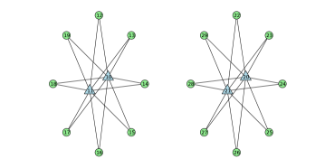
Figure 1: The ‘$2\times 2$’ network. Two ‘roles’, peripheral and central. And two communities also, left and right. The SCF finds the two communities, and the SBM finds the roles.

In all the experiments in this section and the following section, we ran the algorithm for 10,000,000 iterations. By default, we allow the algorithm to select the number of clusters itself as the allocation sampler algorithm naturally searches the entire search space. With this network, the SCF selects $K=2$ and it clusters the nodes into the two star-like communities. The Markov Chain spends 97.5% of its iterations in that ‘ground truth’ state.

On the other hand, the SBM select 4 clusters. It subdivides each of the two true communities into two further communities - one containing the central nodes and the other containing the peripheral nodes. We see this in Figure 2, where very few edges are inside the found clusters. Even if we restrict the SBM to consider only $K=2$, then it again divides the nodes into central and periphery nodes. Regardless of the number of clusters, the SBM finds clusters which do not contain any of the edges; this is the opposite of what we expect in community finding.

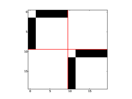
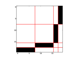
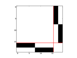
Figure 2: The adjacency matrices showing the clusterings found by the SCF (left) and SBM (middle) on the ‘$2\times 2$’ network (Figure 1). The SCF has found the communities, with all edges inside the clusters, as expected. The SBM has divided the nodes according to degree and community, but there are no edges within any of the four clusters found by the SBM. On the right, we see how the SBM finds only the roles if the number of clusters is fixed at $K=2$ in advance. Only the SCF has placed all the edges inside the clusters and correctly estimated the number of communities.

In networks there may be multiple types of structure that can be detected; the SCF focuses on finding the ‘community-like’ structure, where the clusters are expected to be internally dense. In synthetic and empirical networks with a heavy-tailed degree distribution the SBM may have a tendency to cluster nodes according to their degree, or other structural roles, and not according to community structure.

7 Empirical networks

In this section, we apply the SCF to two well-known social networks.

7.1 Sampson’s Monks

Sampson [13] gathered data on novices at a monastery. There are 18 novices in the network and a pair are linked if they reported a positive friendship between them, giving us an undirected network. There were factions within the group, which Sampson labelled Loyal Opposition, Young Turks and Outcasts.

We ran the SCF method on this dataset for 10,000,000 iterations. It estimated the number of clusters at 3, with 88.5% of the iterations. For 69% of the iterations, the clustering was exactly equal to the factions reported by Sampson. The network and adjacency matrix are shown in Figure 3. We also ran the data through the SBM. It found very similar results. This suggests that if the community structure is strong, then either algorithm can detect it. However, the SBM is slightly less accurate and only 55% of the iterations involve $K=3$. This suggests that there is other structure, perhaps the high-degree versus low-degree structure, that is trying to assert itself.

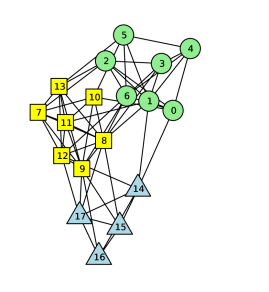
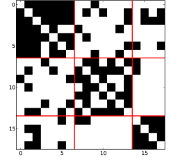
Figure 3: Sampson’s monks, and the 3-way split found by the SCF which matches with the factions found by Sampson.

7.2 Zachary’s Karate club

Now, we apply the SCF to a network of interactions at a karate club [15], again demonstrating the ability of the SCF to detect community structure where the SBM focusses on other types of structure.

The members of the karate club were asked about their social interactions with other members, focusing on interactions outside of the lessons and tournaments. This gives us a network of 34 members and 78 interactions. The interaction data is weighted, according to the number of distinct social interaction types reported by the members; a larger number is taken to indicate a stronger friendship. After the survey was taken, the club split into two factions over a dispute of the cost of the lessons. The network is visualized in Figure 4.

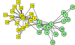
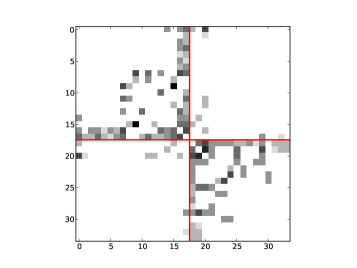
Figure 4: The karate club network of [15]. The width indicates the strength of the relationship by counting the number of distinct interaction types recorded between the two members. The club split in two after the survey and the colour of the node records the split. On the right is the adjacency matrix of this network. The rows and columns have been ordered according to which faction the node is in; most of the edge weight is on the top-left and bottom-right, as would be expected in good community structure. The SCF algorithm finds this clustering when $K=2$.

This network has weighted edges and hence we apply our SCF constraint (eq. 2) to the weighted variant of the SBM. The edges have a Poisson weight, and the rate of the Poisson, $\pi_{kl}$, is different from each block and comes from a Gamma prior; full details of this edge model are in the Appendix of our earlier work[8].

If we fix the number of clusters at $K=2$, then the SCF will correctly cluster the nodes according the split that occured in the club; the chain will spend 85.5% of its iterations in that state. This contrasts with the SBM, which instead clusters the nodes into 9 high-degree and 25 low-degree nodes, a clustering which is quite different from the factional split; this SBM clustering is in Figure 5. The high-degree nodes include the leaders of each faction.

Unfortunately, unlike our earlier networks, the SCF does not correctly estimate the number of clusters within the karate club. We had to specify that $K=2$ in order to find the correct clustering, whereas our MCMC algorithm estimates $K=5$. The issue of model selection within this model may be worth considering further.

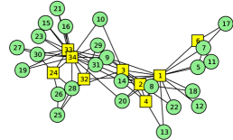
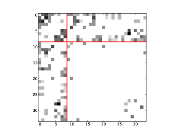
Figure 5: The SBM, when told to find two clusters, divides the nodes according to degree.

8 Conclusion

Community finding is popular in the social science literature, but many statistical models are defined for block-modelling, not explicitly for community-finding. In order to investigate community-finding, we have introduced a constraint that the density inside clusters be larger than the density between pairs of clusters. We have extended an existing block-modelling method, which was based on the Stochastic Block Model (SBM), to take account of this constraint. We evaluated the method and shown it can detect community structure where the SBM cannot.

Acknowledgement

This research was supported by Science Foundation Ireland (SFI) Grant No. 08/SRC/I1407.

References

- Bansal et al. [2004] Bansal, N., Blum, A. & Chawla, S. (2004). Correlation clustering. Machine Learning, 56, 89–113.
- Charikar & Wirth [2004] Charikar, M. & Wirth, A. (2004). Maximizing quadratic programs: Extending grothendieck’s inequality. In 45th Annual IEEE Symposium on Foundations of Computer Science, 54–60, IEEE.
- DasGupta & Desai [2012] DasGupta, B. & Desai, D. (2012). On the complexity of newman’s community finding approach for biological and social networks.
- Daudin et al. [2008] Daudin, J., Picard, F. & Robin, S. (2008). A mixture model for random graphs. Statistical Computing, 18, 173–183.
- Fortunato [2010] Fortunato, S. (2010). Community detection in graphs. Physics Reports, 486, 75 – 174.
- Green [1995] Green, P.J. (1995). Reversible Jump Markov Chain Monte Carlo computation and Bayesian model determination. Biometrika, 82, 711–732.
- Hastings [1970] Hastings, W.K. (1970). Monte Carlo sampling methods using Markov chains and their applications. Biometrika, 57, 97–109.
- McDaid et al. [2012] McDaid, A.F., Murphy, B., Friel, N. & Hurley, N. (2012). Improved Bayesian inference for the Stochastic Block Model with application to large networks.
- Newman & Girvan [2004] Newman, M.E.J. & Girvan, M. (2004). Finding and evaluating community structure in networks. Physical Review E, 69, 026113+.
- Nobile & Fearnside [2007] Nobile, A. & Fearnside, A. (2007). Bayesian finite mixtures with an unknown number of components: The allocation sampler. Statistics and Computing, 17, 147–162.
- Nowicki & Snijders [2001] Nowicki, K. & Snijders, T.A.B. (2001). Estimation and prediction for stochastic blockstructures. Journal of the American Statistical Association, 96, 1077–1087.
- Rosvall & Bergstrom [2008] Rosvall, M. & Bergstrom, C. (2008). Maps of random walks on complex networks reveal community structure. Proc. Natl. Acad. Sci. USA, 105, 1118.
- Sampson [1968] Sampson, S. (1968). A novitiate in a period of change: An experimental and case study of relationships. Unpublished Ph.D. dissertation, Department of Sociology, Cornell University..
- Wyse & Friel [2012] Wyse, J. & Friel, N. (2012). Block clustering with collapsed latent block models. Statistics and Computing, 22, 415–428.
- Zachary [1977] Zachary, W.W. (1977). An information flow model for conflict and fission in small groups. Journal of Anthropological Research, 33, 452–473.
- Zanghi et al. [2008] Zanghi, H., Ambroise, C. & Miele, V. (2008). Fast online graph clustering via Erdős–Rényi mixture. Pattern Recognition, 41, 3592–3599.