Pseudo–potentials based first–principles approach to the magneto–optical Kerr effect: from metals to the inclusion of local fields and excitonic effects

Abstract

We propose a first–principles scheme for the description of the magneto-optical kerr effect within density functional theory (DFT). Though the computation of Kerr parameters is often done within DFT, starting from the conductivity or the dielectric tensor, there is no formal justification to this choice.

As a first steps, using as reference materials iron, cobalt and nickel we show that pseudo–potential based calculations give accurate predictions. Then we derive a formal expression for the full dielectric tensor in terms of the density–density correlation function. The derived equation is exact in systems with an electronic gap, with the possible exception of Chern insulators, and whenever the time reversal symmetry holds and can be used as a starting point for the inclusion of local fields and excitonic effects within time–dependent DFT for such systems.

In case of metals instead we show that, starting from the density–density correlation function, the term which describes the anomalous Hall effect is neglected giving a wrong conductivity.

I Introduction

The Magneto–Optical Kerr Effect (MOKE) consists in the rotation of the polarization plane of light reflected from the surface of a magnetic material. It was discovered in 1877 by John Kerr Kerr1877 ; Kerr1878 while he was examining the light reflected from a polished electromagnet pole. Very recently it became the object of an intense experimental investigations, mainly for two reasons. First one can exploit this effect to read suitably magnetically stored information using optical means in modern high density data storage technology Bertero1994 ; Hatwar1997 . Second, the MOKE can be used as a powerful probe in many fields of research such as microscopy for domain observation, surface magnetism, magnetic interlayer coupling in multilayers Hatwar1997 ; Bennett1990 ; Suzuki1998 ; Zinoni2011 ; Balk2011 . It can also be used to observe plasma resonance effects in thin layers, and structural and magnetic anisotropies Wu1999 ; Zeper1989 ; Weller1992 .

The microscopic origin of the Kerr effect is a combined action of the spin-orbit coupling (SOC) and the net spin–polarization of the material Guo1995 . Indeed the existence of a non zero magnetization in the ground state is due to a spontaneous symmetry breaking of the system. This symmetry breaking is transferred, through the SOC, to the spatial part of the wave–functions so that $\psi_{+L_{z}}(\mathbf{x})$ is different from $\psi_{-L_{z}}(\mathbf{x})$. Accordingly the absorption is different for light with right and left circular polarization.

The problem has been addressed in the literature and ab–initio calculations, based on density functional theory (DFT), are available for transition metals like $Fe$, $Co$ and $Ni$ Delin1999 ; Oppeneer1992 ; Oppeneer1995 ; Guo1995 ; Kim1999 ; Luttinger1967 ; Vernes2002 ; Vernes2004A ; Vernes2004B and, recently, for other materials such as full-Heusler films and $Mn$–doped $GaAs$ Ricci2007 ; Stroppa2008 ; Uba2012 ; Ricci2011 ; Haidu2011 .

The Kerr parameters are commonly obtained from the Kubo formula Kubo1957 for the optical conductivity tensor using the single particle Kohn–Sham (KS) wavefunctions. This is equivalent to the computation of the dielectric constant at the random phase approximation (RPA) without the inclusion of local fields (LF) and exchange–correlation ($xc$) corrections. We will refer to this approach as independent particles RPA (IP–RPA) scheme.

Also an alternative approach, based on the Luttinger’s Formula Luttinger1967 , has been proposed in the literature Vernes2002 ; Vernes2004A ; Vernes2004B , starting from the current–current correlation function, $\underline{\underline{\chi}}_{\mathbf{jj}}$. Also in this case the KS wave–functions are used and LF and xc–effects are not considered.

In all these works the Kerr paramenters are computed within the DFT framework strarting from the dielectric tensor, $\underline{\underline{\varepsilon}}(\omega)$, or, which is the same, from the conductivity, $\underline{\underline{\sigma}}(\omega)$ . However while the diagonal terms of the dielectric tensor, i.e. $\varepsilon_{ii}(\omega)$, can be expressed in terms of the density–density correlation function, $\chi^{0}_{\rho\rho}$ (or $\chi_{\rho\rho}$ if LF and xc effects are included), at the best of our knowledge, no such expression has been derived for the off–diagonal terms, i.e. $\varepsilon_{ij}(\omega)$ with $i\neq j$. The latter can be obtained only starting from $\underline{\underline{\chi}}^{0}_{\mathbf{jj}}$ which however is not expressed as a functional of the density. In this case the sole formal justification to the use of KS quantities to construct $\underline{\underline{\chi}}^{0}_{\mathbf{jj}}$ is that “a posteriori” the approach give good results and that KS wave–functions can be regarded as a good approximation to quasi–particle wave–functions.

In the present work instead we derive an expression for the full dielectric tensor in terms of $\chi^{0}_{\rho\rho}$ and so for the construction of the Kerr parameters within a density based approach. Besides a formal justification to the use of the DFT approach, the result we propose can be regarded as a starting point to go beyond the RPA–IP scheme to include LF and xc–effects. Indeed while the description of transition metals within the RPA–IP approach is reasonable, for semiconductors important deviations are expected, in particular when excitons (magnetic excitons) exist. Magnetic semiconductors are in fact materials of great interest, especially in view of spin electronics (spintronics) applications and the MOKE can be a valuable tool for the investigation of their properties Acbas2009 ; Sun2011 .

In the present work we limit our discussion to the polar geometry, that is when the propagation direction of the photon (the $z$ axis) and the magnetization of the system are both perpendicular to the surface of the sample ($xy$). Experimentally this is the most studied geometry, and it is also the one which in general gives the largest MOKE signal. To support our theoretical derivation with numerical results we have implemented in the plane–waves and pseudo–potentials based code $Yambo$ Yambo the computation of the Kerr parameters. We have tested our implementation in transition metals for which well assessed all electrons calculations and experimental results are available. For these materials the IP–RPA approximation is sufficient.

Thus in Sec. II we show results on bulk iron, cobalt and nickel in order to validate our pseudo–potential based approach, at the IP–RPA level.

Then we discuss how to construct a formal equation for the dielectric tensor starting from $\chi^{0}_{\rho\rho}$ in Sec. III. This approach is compared with the one based on $\underline{\underline{\chi}}^{0}_{\mathbf{jj}}$. The two differ by a term which, in general, is zero in systems with an electronic gap or whenever the pure time reversal symmetry holds. This term describes the anomalous Hall conductivity. Taking iron as reference system we show that, neglecting this term, a large error is induced in the computation of the off diagonal conductivity in metals. However the anomalous Hall conductivity is zero in systems with an electronic gap footnote_chern , thus our approach is exact for dielectrics. We then show how LF and xc–effects can be included replacing $\chi^{0}_{\rho\rho}$ with $\overline{\chi}_{\rho\rho}$. The results is a scheme, in principle exact, to compute the Kerr parameters within time–dependent DFT (TDDFT).

II Moke parameters with the IP–RPA approximation

II.1 Theoretical background

The description of the MOKE can be obtained in terms of the dielectric function $\varepsilon(\omega)$ or equivalently of the optical conductivity $\sigma(\omega)$. The two are related by the equation

$$\underline{\underline{\sigma}}(\omega)=\frac{\omega}{4\pi i}(\underline{\underline{\varepsilon}}(\omega)-\underline{\underline{1}})\text{,}$$ (1)

where the dielectric tensor at the IP–RPA level can be constructed from the (paramagnetic) $\chi^{0}_{\textbf{jj}}$, according to the equation Strinati1988 :

$$\varepsilon_{\alpha,\beta}(\omega)=\left(1-\frac{4\pi e^{2}n}{m\omega^{2}}\right)\delta_{\alpha,\beta}-\frac{4\pi e^{2}}{\omega^{2}}\ \chi^{0}_{j_{\alpha}j_{\beta}}(\mathbf{0},\omega)\text{.}$$ (2)

Here $e$ is the electron charge and $m$ the electron mass, $\Omega$ the unit cell volume, $\alpha$ labels the Cartesian axis, and $n=N_{el}/\Omega$ the number of electrons per unit volume. The IP response functions is:

$$\chi^{0}_{j_{\alpha}j_{\beta}}(\mathbf{q},\omega) = \sum_{cv}\int\frac{d^{3}\mathbf{k}}{(2\pi)^{3}}\left[\chi^{0}_{j_{\alpha}j_{\beta}}(\mathbf{k},\omega)\right]_{cv\mathbf{kq}}$$ (3)

$$= \frac{1}{m^{2}}\sum_{cv}\int\frac{d^{3}\mathbf{k}}{(2\pi)^{3}}\left[\frac{(p_{cv\mathbf{k}}^{\alpha}(\mathbf{q}))^{*}p_{cv\mathbf{k}}^{\beta}(\mathbf{q})\ f_{v\mathbf{k}}(1-f_{c\mathbf{k-q}})}{\hbar\omega-(\epsilon_{c\mathbf{k-q}}-\epsilon_{v\mathbf{k}})+i\eta}-\right.$$

$$\phantom{\sum_{cv}\int\frac{d^{3}\mathbf{k}}{(2\pi)^{3}}\left[\chi^{0}_{j_{\alpha}j_{\beta}}(\mathbf{q},\omega)\right]_{cv\mathbf{kq}}}\left.\frac{(p_{vc\mathbf{k}}^{\alpha}(\mathbf{q}))^{*}p_{vc\mathbf{k}}^{\beta}(\mathbf{q})\ f_{v\mathbf{k-q}}(1-f_{c\mathbf{k}})}{\hbar\omega+(\epsilon_{c\mathbf{k}}-\epsilon_{v\mathbf{k-q}})+i\eta}\right],$$

where the first term on the r.h.s. is the resonant part, while the second in the anti-resonant one. $c$ ($v$) are conduction (valence) band indexes, $f_{i\mathbf{k}}$ are the occupation factors, $\epsilon_{i}({\bf k})$ the electronic energy at ${\bf k}$ and $p_{cv\mathbf{k}}^{\alpha}(\mathbf{q})$ the expectation value of the momentum operator ${\langle c\mathbf{k-q}|\hat{p}^{\alpha}|v\mathbf{k}\rangle}$ which in our pseudo–potential based scheme must be computed as Read1991

$$\langle c\mathbf{k-q}|\left(\hat{p}^{\alpha}-\frac{im}{\hbar}[\hat{x}^{\alpha},\hat{V}_{NL}]\right)|v\mathbf{k}\rangle\text{,}$$ (4)

where $\hat{x}^{\alpha}$ is the $\alpha$ component of the position operator and $V_{NL}$ the non–local part of the pseudo–potential. The infinitesimal $\eta$ factor implies that the electromagnetic field is adiabatically turned on at $t=-\infty$ but can also be viewed as a finite lifetime broadening which accounts for scattering process and finite experimental resolution. In the present work we use $\eta(\omega)=0.3\ eV+0.03\hbar\omega$ to mimic an experimental resolution which decrease linearly with energy as in Ref. Delin1999, .

II.2 MOKE spectra for transition metals

As a first step we check how a pseudo–potentials based approach preforms in the description of the Kerr parameters, as it is common wisdom Delin1999 that all electrons calculation are needed to describe the wave–function in the core region, where the SOC is mostly effective, and thus to evaluate the MOKE.

We start from a ground state DFT calculation for bulk iron, cobalt and nickel with the $Abinit$ code Abinit , using norm–conserving HGH HGH pseudo–potentials and including the SOC; we found out that it is crucial, for a correct description of the MOKE, to have the SOC effect included both in the pseudo–Hamiltonian and in the construction of the pseudo–potential.

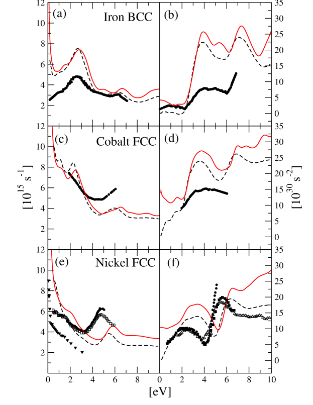
Figure 1: (color online) Plot of $\sigma_{xx}(\omega)$ for bulk BCC iron (Panels $a$-$b$), bulk fcc cobalt (Panels $c$-$d$) and bulk fcc nickel (Panels $a$-$b$). The continuous (red) line are the results from the preset work. The dashed line are all electrons results from Ref. Delin1999, . The symbols are experimental measurements. Panels $a$-$b$: Ref. Johnson1974, . Panels $c$-$d$: Ref. Nakajima1996, . Panels $e$-$f$: filled circels, Ref. Nakajima1996, ; empty squares, Ref. Shiga1969, ; filled triangles, Ref. Stoll1971, ; filled squares, Ref. Johnson1974, ; empty triangles, Ref. Ehereinreich1963, .

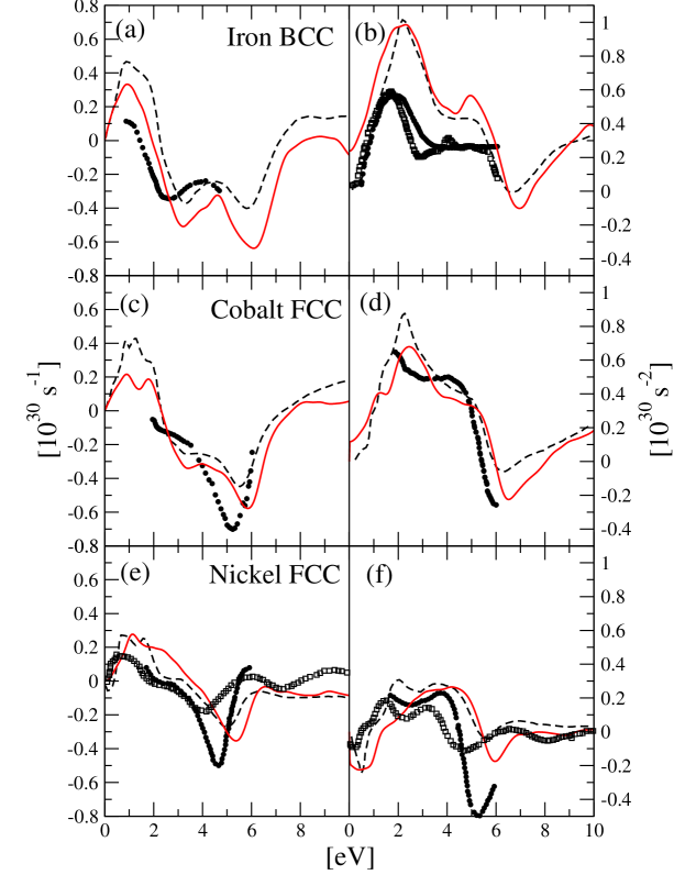
Figure 2: (color online) Plot of $\sigma_{xy}(\omega)$ for bulk BCC iron (Panels $a$-$b$), bulk fcc cobalt (Panels $c$-$d$) and bulk fcc nickel (Panels $a$-$b$) The continuous (red) line are the results from the preset work. The dashed line are all electrons results from Ref. Delin1999, . The symbols are experimental measurements. Panels $a$-$b$: filled circles, Ref. Engen1983, ; empty squares, Ref. Krinchik1968, . Panels $c$-$d$: Ref. Nakajima1996, . Panels $e$-$f$: filled circels, Ref. Nakajima1996, ; empty squares, Ref. Erskine1977, .

Bulk iron is studied in its bcc phase with the experimental cell parameter $a=2.87$ Å; an energy cutoff of 65 $Ha$ and a k–points sampling of the Brillouin zone (BZ) 14x14x14. Bulk cobalt is studied in its fcc phase with the experimental cell parameter $a=3.55$ Å; an energy cutoff of 55 $Ha$ and a k–points sampling of the BZ 8x8x8. Finally bulk nickel is studied in its fcc phase with the experimental cell parameter $a=3.52$ Å; an energy cutoff of 65 $Ha$ and a k–points sampling of the BZ zone 14x14x14. Semi–core electrons are also included in the pseudo–potentials for all systems, as we found the density of states to be poorly described using the HGH pseudo–potentials with only valence electrons, constructed from the parameters of Ref. HGH, .

Then we compute the dielectric function with the $Yambo$ code Yambo according to a modified version of Eq. 2:

$$\varepsilon_{\alpha,\beta}(\omega)=\left(1+\frac{4\pi e^{2}}{\omega^{2}}\chi^{0}_{j_{\alpha}j_{\beta}}(\mathbf{0},0)\right)\delta_{\alpha,\beta}-\frac{4\pi e^{2}}{\omega^{2}}\ \chi^{0}_{j_{\alpha}j_{\beta}}(\mathbf{0},\omega)\text{.}$$ (5)

where the diamagnetic term has been replaced by the zero frequency value of $\chi_{jj}$. Indeed in cold semi–conductors the diamagnetic term must be exactly balanced by $\chi^{0}_{j_{\alpha}j_{\beta}}(\mathbf{0},0)$, due to the effective–mass sum rule Sipe1993 ; Virk2007 ; Giuliani2005 , but this balance is slowly converging with the number of $cv$ states included and the use of $\chi^{0}_{j_{\alpha}j_{\beta}}(\mathbf{0},0)$ speeds up the convergence footnote_Drude . In metals instead the difference between the diamagnetic term and the zero frequency value of $\chi_{jj}$ gives the Drude term, which, with this choice, is set to zero. However it has been shown Marini2001 that in practice a ultra–fine sampling of the BZ would be needed to compute this difference. Hence it is preferable to include it with a semi–classical model as described in Ref. Marini2001, . The Drude term is included only in the computation of the diagonal part of $\underline{\underline{\varepsilon}}(\omega)$. The optical conductivity is finally constructed from Eq. 1. Here for the Drude term we used the same parameters of the reference all–electrons calculation, i.e. ${\omega_{P}=(4.9+i1.8\pi)\ eV}$ for iron, $\omega_{P}=(8.3+i2\pi)\ eV$ for cobalt and $\omega_{P}=(7.5+i2.24\pi)\ eV$ for nickel.

The results for the optical conductivity are plotted in Figs. 1-2. For all systems there is a systematic blue shift of the theoretical peaks against the experimental data. This is a known problem of the LDA, due to the self–interaction error, which tends to delocalize the $d$–orbitals and accordingly gives wrong eigenvalues. The same consideration also explains the overestimation of the intensity, as delocalization increases the orbitals overlap and thus the intensity of the dipoles computed to construct the dielectric function. However a good agreement is found with the reference all–electrons calculations. The diagonal component, $\sigma_{xx}(\omega)$, is commonly computed from pseudo–potential based calculations, provided that the dipoles are constructed as in Eq. 3. For the off–diagonal component, $\sigma_{xy}(\omega)$, instead, it has been reported that it must be computed using all–electrons wavefunctions Delin1999 , because it depends crucially on the correction to the wave–function due to the SOC term in the Hamiltonian. However, in our results, the differences in the diagonal and the off–diagonal part of the optical conductivity compared to the reference all–electrons calculations are of the same order. Hence we can conclude that pseudo–potentials based calculation can be used to compute the Kerr parameters with the same level of confidence of absorption spectra, which depend only on the diagonal part of the optical conductivity. We mention that, in the literature, pseudo–wavefunctions has been used to construct the off–diagonal conductivity at $\omega=0$ in the computation of the anomalous Hall conductivity Yafet2007 ; Wang2006 ; Wang2007 . Also in this case a good agreement with the all–electrons calculations was found.

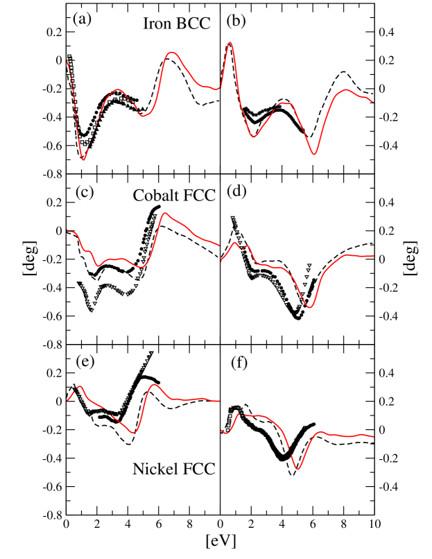
Figure 3: (color online) Plot of the Kerr paramenters $\Psi_{K}(\omega)=\theta_{K}+i\gamma_{K}$ for bulk BCC iron (Panels $a$-$b$), bulk fcc cobalt (Panels $c$-$d$) and bulk fcc nickel (Panels $a$-$b$). The continuous (red) line are the results from the preset work. The dashed line are all electrons results from Ref. Delin1999, . The symbols are experimental measurements. Panels $a$-$b$: filled circles, Ref. Engen1983, ; empty diamonds, Ref. Krinchik1968, ; empty triangles, Ref. Katayama1986, ; stars, Ref. Visnovsky1996, ; filled squares, Ref. Kawagoe1992, . Panels $c$-$d$: filled circels, Ref. Nakajima1996, ; empty triangles, Ref. Weller1994, . Panels $e$-$f$: filled circels, Ref. Nakajima1996, ; empty triangles, Ref. Krinchik1968, ; Empty squares, Ref. Engen1983, .

Thus we finally compute the complex Kerr parameters according to the equation

$$\Psi_{K}(\omega)=\theta_{K}(\omega)+i\gamma_{K}(\omega)=\frac{-\varepsilon_{xy}}{(\varepsilon_{xx}-1)\sqrt{\varepsilon_{xx}}}\text{,}$$ (6)

which is the standard expression for the polar geometry in the small angles limit. Here the photon propagates along the $z$ direction and describes a linearly polarized wave with the electric field along the $x$ direction. Results are reported in Fig. 3. The blue shift of the theoretical results is still present, while the overestimation of the dipoles in both $\sigma_{xx}(\omega)$ and $\sigma_{xy}(\omega)$ is compensated and the intensity of the MOKE signal is closer to the experimental data than for the case of the optical conductivity.

To conclude this section, we have shown that for $Fe$, $Co$ and $Ni$ the Kerr computed from our pseudo–potential approach are in good agreement with the results obtained from all–electrons calculations.

III Beyond the IP–RPA approximation

III.1 A density based approach.

In the previous section we have constructed the Kerr paramenters starting from the KS wave–functions using Eq. 2, as it is commonly done in the literature. However the use of KS wave–function to construct $\underline{\underline{\chi}}^{0}_{\mathbf{jj}}$ is not formally justified. Moreover the inclusion of LF and xc effects within a density based approach in Eq. 2 is not straightforward.

However, to describe the MOKE only the long wave–length term, i.e. $\mathbf{q}=0$, of the dielectric function is needed, where the distinction between longitudinal and transverse fields disappears. In this limit the diagonal part of the dielectric tensor can be constructed from $\chi^{0}_{\rho\rho}$ which, at finite $\mathbf{q}$, describes only the longitudinal term of the dielectric tensor. This approach is formally justified within a density based approach and moreover would allow a straightforward inclusion of LF and xc effects within the TDDFT scheme. It is then tempting to try to construct the full dielectric tensor at $\mathbf{q}=0$ from $\chi^{0}_{\rho\rho}$ and use the result to go beyond the IP–RPA scheme.

Here we provide an heuristic derivation where only longitudinal fields are considered, as our final goal is to take the $\mathbf{q}\rightarrow 0$ limit. We will prove a posteriori that the result is correct for systems with an electronic gap or, more in general, when the pure time–reversal symmetry exist and we will discuss in detail the difference between the derived equation and Eq. 2.

We consider a non uniform system. The dielectric function is defined as:

$$\mathbf{E}^{ext}(\mathbf{q},\omega)=\underline{\underline{\varepsilon}}(\mathbf{q}\mathbf{q^{\prime}},\omega)\mathbf{E}^{tot}(\mathbf{q^{\prime}},\omega)\text{.}$$ (7)

Assuming that only longitudinal fields exist, Eq. (7) can be written in terms of the potentials

$$V^{ext}(\mathbf{q},\omega)=\mathbf{\hat{q}}\ \underline{\underline{\varepsilon}}(\mathbf{q}\mathbf{q^{\prime}},\omega)\ \mathbf{\hat{q}^{\prime}}V^{tot}(\mathbf{q^{\prime}},\omega),$$ (8)

where the two are related by the equation

$$V^{ext}(\mathbf{q},\omega) = V^{tot}(\mathbf{q},\omega)-V^{ind}(\mathbf{q},\omega)=$$ (9)

$$= V^{tot}(\mathbf{q},\omega)-\frac{4\pi e^{2}}{q^{2}}\chi^{0}_{\rho\rho}(\mathbf{q},\mathbf{q^{\prime}},\omega)V^{tot}(\mathbf{q^{\prime}},\omega)\text{.}$$ (10)

Inserting Eq. 10 into Eq. 8 and taking the limit $\mathbf{q}\rightarrow\mathbf{q^{\prime}}\rightarrow 0$ we can define a generalization of the relation that holds between $\varepsilon_{\alpha\alpha}$ and $\chi_{\rho\rho}$ Strinati1988 :

$$\varepsilon_{\alpha\beta}(\omega)=\delta_{\alpha\beta}-\lim_{q_{\alpha},q_{\beta}\rightarrow 0}\frac{4\pi e^{2}}{q^{2}}\chi^{0}_{\rho\rho}(q_{\alpha},q_{\beta},\omega)\text{.}$$ (11)

In order to compare Eq. 11 and Eq. 2 we first notice that the latter is divergent for $\omega\rightarrow 0$. After some algebra Eq. 2 can be rewritten as Sipe1993 :

$$\varepsilon_{\alpha,\beta}(\omega)=\frac{A_{\alpha\beta}}{\omega^{2}}+\frac{B_{\alpha\beta}}{\omega}+\delta_{\alpha\beta}+\sum_{cv}\frac{d^{3}\mathbf{k}}{(2\pi)^{3}}\ \frac{4\pi e^{2}\hbar^{2}}{(\epsilon_{c\mathbf{k}}-\epsilon_{v\mathbf{k}})^{2}}\ \left[\chi^{0}_{j_{\alpha}j_{\beta}}(\mathbf{0},\omega)\right]_{cv\mathbf{k0}}\text{.}$$ (12)

$A_{\alpha\beta}$ describes the contribution from the electrons at the Fermi surface, i.e. the Drude term, and is zero in cold semiconductors, when there are not partially filled bands. This term is also included in Eq. 11 in the $q\rightarrow 0$ limit as discussed in Ref. Marini2001, . Once the $\omega^{-2}$ has been isolated using the relation $x^{\alpha}_{cv\mathbf{k}}=-i\hbar p^{\alpha}_{cv\mathbf{k}}/(m(\epsilon_{c\mathbf{k}}-\epsilon_{v\mathbf{k}}$)) in the last term of Eq. 12 together with

$$\lim_{\mathbf{q,q^{\prime}}\rightarrow 0}\chi^{0}_{\rho\rho}(\mathbf{q,q^{\prime}},\omega) = \lim_{\mathbf{q,q^{\prime}}\rightarrow 0}\sum_{c\ v}\int d^{3}\mathbf{k}\left[\frac{(i\mathbf{q}\cdot\mathbf{x}_{cv\mathbf{k}}^{*})(i\mathbf{q^{\prime}}\cdot\mathbf{x}_{cv\mathbf{k}})\ f_{v\mathbf{k}}(1-f_{c\mathbf{k-q}})}{\hbar\omega-(\epsilon_{c\mathbf{k-q}}-\epsilon_{v\mathbf{k}})+i\eta}-\right.$$ (13)

$$\phantom{\chi^{0}_{\rho\rho}(\mathbf{q},\omega)=\sum_{cv}\int d^{3}\mathbf{k}}\left.\frac{(i\mathbf{q}\cdot\mathbf{x}_{vc\mathbf{k}}^{*})(i\mathbf{q^{\prime}}\cdot\mathbf{x}_{vc\mathbf{k}})\ f_{v\mathbf{k-1}}(1-f_{c\mathbf{k}})}{\hbar\omega+(\epsilon_{c\mathbf{k}}-\epsilon_{v\mathbf{k-q}})+i\eta}\right],$$

we obtain the remaining part of Eq. 11.

III.2 The anomalous Hall effect

Hence term $B_{\alpha\beta}$ is not included in Eq. 11. It can be explicitly written, at the RPA-IP level, as:

$$B_{\alpha\beta}=\frac{\hbar e^{2}}{2\pi^{2}m^{2}}\sum_{uw}\int d^{3}\mathbf{k}(f_{u\mathbf{k}}-f_{w\mathbf{k}})\frac{(p_{wu\mathbf{k}}^{\alpha})^{*}p_{wu\mathbf{k}}^{\beta}}{(\epsilon_{w\mathbf{k}}-\epsilon_{u\mathbf{k}})^{2}}\text{.}$$ (14)

This can be shown to be zero when the time–reversal symmetry holds Sipe1993 or in any case when ${\alpha=\beta}$ inverting the mute indexes $u$ and $w$ in the second term on the r.h.s. . In MOKE experiments however the time–reversal is broken by the existence of a ground state magnetization and by the SOC term in the Hamiltonian and for the construction of $\Psi_{K}(\omega)$ we need the terms ${\alpha\neq\beta}$.

Thus $B_{\alpha\beta}$ can differ from zero. In the following, we briefly discuss its physical meaning. To fix the ideas we chose $\alpha=x$ and $\beta=y$. It can be easily proved that the the $B_{xy}$ coefficient is (apart a trivial factor raising from the relation between $\underline{\underline{\varepsilon}}$ and $\underline{\underline{\sigma}}$) the intrinsic anomalous Hall conductivity (AHC), which is responsible of anomalous Hall effect in magnetic metals.

In fact, according to Ref. Yao2004 the AHC reads

$$\sigma^{AHC}_{xy}=-\frac{e^{2}}{\hbar}\sum_{u}\int\frac{d^{3}{\bf k}}{(2\pi)^{3}}f_{u{\bf k}}\Omega^{z}_{u}({\bf k});$$ (15)

i.e. $\sigma^{AHC}$ can be expressed as a BZ integral of the Berry curvature of the $u$-band, $\Omega^{z}_{u}({\bf k})$ (summed over all the occupied states). The latter quantity can be written in terms of the ingredients of Eq. 14 as:Yao2004

$$\Omega^{z}_{u}({\bf k})=-\frac{\hbar^{2}}{m^{2}}\sum_{w,w\neq u}\frac{2Im\left(p^{x}_{uw\mathbf{k}}p^{y}_{wu\mathbf{k}}\right)}{\left(\epsilon_{u{\bf k}}-\epsilon_{w{\bf k}}\right)^{2}}$$ (16)

After some straightforward algebra, one can easily prove that the AHC can be expressed as

$$\sigma^{AHC}_{xy}=\frac{B_{xy}}{4\pi i};$$ (17)

which provide the relations between $B$ and the AHC. In the case of magnetic metals, our expression constitute an alternative approach to compute $\sigma^{AHC}$ with respect to the methods based on the computation of Berry phase Wang2007 . In the case of insulators instead $\sigma^{AHC}$ has been recognized as a topological invariant Thouless1982 , also called Chern number, which can take only integer values Thus, in dielectric, $B_{xy}$ can be non-zero only in the so-called Chern insulator, hypothetical materials showing a quantum Hall effect without external magnetic field. In practice for all the presently known dielectrics eq. 11 can be considered exact.

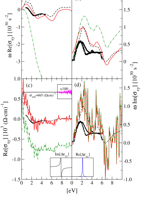
Figure 4: (color online) Off–diagonal element of the conductivity tensor, $\sigma_{xy}(\omega)$, of iron computed starting from Eq. 11, dot–dashed (green) line and from Eq. 2 continuous (red) line. The dashed line are all electrons results from Ref. Delin1999, . The symbols are experimental measurements: filled circles, Ref. Engen1983, ; empty squares, Ref. Krinchik1968, . In panels $a$-$b$ $\sigma_{xy}(\omega)$ is computed with the smearing used in the present work. In panels $c$ and $d$ instead $\sigma_{xy}(\omega)$ is evaluated at $\eta=0.05\ eV$. The difference between the dot–dashed (green) line and the continuous (red) line is represented with a thin (black) line. In the inset of the panels also the difference in terms of the dielectric function is represented.

Also in this case we have tested, at the IP–RPA level, the effect of $B_{\alpha\beta}$ on bulk iron comparing the conductivity computed starting either from Eq. 2 or from Eq. 11. In Fig. 4.$(a-b)$ we show the error induced in the computation of the off-diagonal conductance on bulk iron.

To clarify the relation between this difference and the AHC also numerically we have considered, in Fig. 4.$(c-d)$, the plot of the conductivity at small smearing, i.e. $\eta=0.05\ eV$, as Eq.2 and Eq. 11 are equal only in the limit $\eta\rightarrow 0\$ footnote_eta . From Fig. 4.$(c)$ is clear that the difference of the two gives a constant value, as expected theoretically, a part from the region $\omega\simeq 0$, where the $1/\omega^{2}$ term makes Eq. 2 numerically unstable. We can thus extract the $\sigma_{xy}^{AHC}=665\ (\Omega cm)^{-1}$ which is not so far from the theoretically computed value $750.8\ (\Omega cm)^{-1}$ of Ref. Yao2004, . The difference is likely due to the sampling of the BZ. As for the case of the Drude term, the anomalous Hall conductivity depends on the contribution from the electrons at the Fermi surface and thus a very fine sampling of the BZ should be needed, which is beyond the scope of the present work. Also we see in Fig. 4.$(d)$ that at small $\eta$ the difference between the imaginary parts of the conductivity computed with the two approaches goes to zero (Fig. 4.$(b)$) as expected from the theoretical derivation. Finally in the insets we have also represented the difference at the level of the dielectric function which are $Im[\Delta\varepsilon]\propto 1/\omega$ and $Re[\Delta\varepsilon]\propto\delta(\omega)$ thus respecting the Krames–Kronig relations.

III.3 Inclusion of local fields and excitonic effects.

The generalization of Eq. 2 to include LF and $xc$–effects is non trivial and needs a careful distinction between longitudinal and transverse induced fields. The result, derived in Ref. [DelSole1984, ], is to replace the IP $\underline{\underline{\chi}}^{0}_{\mathbf{jj}}$ with the one constructed from the analytical part of the electron–hole ($eh$) propagator $\overline{L}(12,34)$ solution of the modified Bethe–Salpeter equation:

$$\overline{L}(12,34)=L_{0}(12,34)+L_{0}(12,1^{\prime}2^{\prime})\\ \Big{[}\overline{v}(1^{\prime},3^{\prime})\delta(1^{\prime},2^{\prime})\delta(3^{\prime},4^{\prime})-iW(1,2)\delta(1^{\prime},3^{\prime})\delta(2^{\prime},4^{\prime})\Big{]}\overline{L}(3^{\prime}4^{\prime},34),$$ (18)

with $1$ representing spatial, time and spin coordinates: $1=(\mathbf{x_{1}},t_{1},\sigma_{1})$. The long range part of the exchange interaction ${v(1,2)=\delta(t_{1}-t_{2})/|\mathbf{x_{1}-x_{2}}|}$ between the electron and the hole is truncated with the substitution $v\rightarrow\overline{v}$ where in reciprocal space

$$\overline{v}_{\mathbf{G}}(\mathbf{q})=\begin{cases}4\pi e^{2}/|\mathbf{q+G}|^{2}&\text{if $\mathbf{G\neq 0}$,}\\ 0&\text{if $\mathbf{G=0}$.}\end{cases}.$$ (19)

From the electron–hole propagator the $\underline{\underline{\overline{\chi}}}_{\mathbf{jj}}$ and $\underline{\underline{\overline{\chi}}}_{\rho\rho}$ are constructed with the relations Strinati1988

$$\overline{\chi}_{\rho\rho}(1,2) = -i\hbar\overline{L}(1,2;1^{+},2^{+}),$$ (20)

$$\underline{\underline{\overline{\chi}}}_{\mathbf{jj}}(1,2) = -i\hbar\frac{-\hbar^{2}}{4m^{2}}\left[\mathbf{(\nabla_{1}-\nabla_{1}^{\prime})(\nabla_{2}-\nabla_{2}^{\prime})}\overline{L}(1,2;1^{\prime}2^{\prime})\right]_{1^{\prime}=1^{+},2^{\prime}=2^{+}}\text{,}$$ (21)

with $1^{+}=lim_{\tau\rightarrow 0}(\mathbf{x_{1}},t_{1}+\tau,\sigma_{1})$ The result is then

$$\varepsilon_{\alpha,\beta}(\omega)=\left(1-\frac{4\pi e^{2}n}{m\omega^{2}}\right)\delta_{\alpha,\beta}-\frac{4\pi e^{2}}{\omega^{2}}\ \overline{\chi}_{j_{\alpha}j_{\beta}}(\mathbf{0},\omega)\text{.}$$ (22)

A possible strategy to remain within a density based formalism footnote_RealTime_DFT , starting from Eq. 2, could be to use the unphysical $L^{TDDFT}$ replacing $iW(1,2)\delta(1^{\prime},3^{\prime})\delta(2^{\prime},4^{\prime})$ with $f_{xc}(1,2)\delta(1^{\prime},2^{\prime})\delta(3^{\prime},4^{\prime})$ in Eq. 18. However this is not formally justified neither and at least a current based formalism should be used, i.e. current–DFT Vignale1987 ; Vignale2004 ; Abedinpour2010 . Indeed for the description of absorption spectra, the diagonal part only of the dielectric function is commonly constructed from $\overline{\chi}_{\rho\rho}$ to include LF and xc effects footnote_G0 starting from $\varepsilon_{ii}(\omega)[\chi^{0}_{\rho\rho}]$. A similar derivation can be used to include LF and xc–effects replacing ${\chi^{0}_{\rho\rho}}$ with ${\overline{\chi}_{\rho\rho}}$ in Eq. 11. In this case however the Dyson equation for the response function should be written for a non homogeneous system assuming, as we did in the IP case, that transverse fields can be neglected as we are looking for the $\mathbf{q}\rightarrow 0$ limit. The result is:

$$\varepsilon_{\alpha\beta}(\omega)=\delta_{\alpha\beta}-\lim_{q_{\alpha},q_{\beta}\rightarrow 0}\frac{4\pi e^{2}}{q^{2}}\overline{\chi}_{\rho\rho}(q_{\alpha},q_{\beta},\omega)\text{,}$$ (23)

which, according to the discussion of the previous sections should hold when the time–reversal symmetry exists or for systems with an electronic gap footnote_chern ; footnote_future . Eq. 23 must then be compared with Eq. 22. If $\overline{\underline{\underline{\chi}}}_{\mathbf{jj}}$ and $\overline{\chi}_{\rho\rho}$ are constructed from the same $\overline{L}$ using Eqs. 20-21 the two are diagonalized by the same vectors in $c\ v$ space, $A^{I}_{cv\mathbf{k}}$; here $I$ is the index of the excitation, which now can be a mixture of electron–hole pairs. In this case inserting the vectors $A^{I}_{cv\mathbf{k}}$ in the equations the two approach will differ by the term

$$B_{\alpha\beta}=\frac{\hbar e^{2}}{2\pi^{2}m^{2}}\sum_{I}\sum_{uw}\int d^{3}\mathbf{k}(f_{u\mathbf{k}}-f_{w\mathbf{k}})\frac{(A^{I}_{wu\mathbf{k}}p_{wu\mathbf{k}}^{\alpha})^{*}A^{I}_{wu\mathbf{k}}p_{wu\mathbf{k}}^{\beta}}{(\hbar\omega_{I})^{2}}\text{,}$$ (24)

which defines a generalization of the Anomalous Hall effect. Here $\omega_{I}$ are the poles of $\overline{\chi}_{\rho\rho}$. In common metals usually we have $A^{I}_{cv\mathbf{k}}=\delta_{I,(cv)_{I}}$ (i.e. each vector $A^{I}$ is different from zero only for a specific transition $cv=(cv)_{I}$ ) and $\hbar\omega_{I}=\epsilon_{ck}-\epsilon_{vk}$, thus Eq. 24 reduces to Eq. 14.

However if one remains within a pure DFT approach, then the vectors which diagonalize $\overline{\chi}_{\rho\rho}$, $A^{I,TDDFT}_{cv\mathbf{k}}$ do not, in general, diagonalize $L$ and thus $\overline{\underline{\underline{\chi}}}_{\mathbf{jj}}$. In this case Eq. 23 and Eq. 22 could also differ by a term proportional to $A^{I,TDDFT}_{cv\mathbf{k}}-A^{I}_{cv\mathbf{k}}$. This term must be zero for $\alpha=\beta$, while its relevance in the case $\alpha\neq\beta$ and its eventual physical meaning are left under study.

IV Conclusions

We have proposed a scheme to compute the magneto–optical Kerr effect in magnetic–semiconductors. The scheme has two main novelties. First is based on pseudo–potentials calculations. This is the most widely used approach to describe extended systems and we have shown that pseudo–wavefunctions can be used to obtain the Kerr parameters. The results we find are comparable with all–electrons calculations, provided that the Spin–Orbit interaction is correctly accounted for in the construction of the pseudo–potential.

Second we have discussed the inclusion of local–field and excitonic effects in the computation of the MOKE. We have shown that two strategies can be used: (i) the Bethe–Salpeter equation, through the result derived in Ref. DelSole1984, , but also, in almost any case of interest, (ii) an approach based on time–dependent density–functional theory and in general on the density–density correlation function through the result derived in the present manuscript.

V Acknowledgments

This work was partially funded by the Cariplo Foundation through the Oxides for Spin Electronic Applications (OSEA) project (n. 2009-2552). D. Sangalli would like to acknowledge G. Onida and the European Theoretical Spectroscopy Facility ETSF (ETSF) Milan node for the opportunity of running simulations on the ETSF–Milano (ETSFMI) cluster, and P. Salvestrini for technical support on the cluster. We also acknowledge computational resources provided by the Consorzio Interuniversitario per le Applicazioni di Supercalcolo Per Universitá e Ricerca (CASPUR) within the project MOSE. Finally D. Sangalli and A. Debernardi would like to thank R. Colnaghi for technical support.

References

- (1) J. Kerr, Philos. Mag. 3, 321 (1877)
- (2) J. Kerr, Philos. Mag. 5, 161 (1878)
- (3) G. A. Bertero, and R. Sinclair, J. Magn. Magn. Mater. 134, 173 (1994)
- (4) T. K. Hatwar, Y. S. Tyan, and C. F. Bruker, J. Appl. Phys. 81, 3839 (1997)
- (5) R. Alcaraz de la Osa, J. M. Saiz, F. Moreno, P. Vavassori, and A. Berger, Phys. Rev. B 85, 064414 (2012)
- (6) W. R. Bennett, W. Schwarzacher, and W. F. Egelhoff, Phys. Rev. Lett. 65, 3169 (1990)
- (7) Y. Suzuki, T. Katayama, P. Bruno, S. Yuasa, and E. Tamura, Phys. Rev. Lett. 80, 5200 (1998)
- (8) C. Zinoni, A. Vanhaverbeke, P. Eib, G. Salis, and R. Allenspach, Phys. Rev. Lett. 107, 207204 (2011)
- (9) A. L. Balk, M. E. Nowakowski, M. J. Wilson, D. W. Rench, P. Schiffer, D. D. Awschalom, and N. Samarth, Phys. Rev. Lett. 107, 077205 (2011)
- (10) R. Q. Wu, and A. J. Freeman, J. Magn. Magn. Mater. 200, 498 (1999)
- (11) W. B. Zeper, F. J. A. M. Greidanus, P. F. Garcia, and C. R. Fincher, J. Appl. Phys. 65, 4971 (1989)
- (12) D. Weller, H. Brändle, G. Gorman, C.-J. Lin, and H. Notarys, Appl. Phys. Lett. 61, 2726 (1992)
- (13) G. Acbas, M.-H. Kim, M. Cukr, V. Novàk, M. A. Scarpulla, O. D. Dubon, T. Jungwirth, Jairo Sinova, and J. Cerne, Phys. Rev. Lett. 103, 137201 (2009)
- (14) C. Sun, J. Kono, A. Imambekov, and E. Morosan, Phys. Rev. B 84, 224402 (2011)
- (15) A. Marini, C. Hogan, M. Grüning, and D. Varsano, Comp. Phys. Comm. 180, 1392 (2009)
- (16) With the exception of the so-called Chern insulator.
- (17) G. Y. Guo, H. Ebert, Phys. Rev. B 51, 12633 (1995)
- (18) A. Delin, O. Eriksson, B. Johansson, S. Auluck, and J. M. Wills, Phys. Rev. B 60, 14105 (1999)
- (19) P. M. Oppeneer, T. Maurer, J. Sticht, and J. Kübler, Phys. Rev. B 45, 10924 (1992)
- (20) P. M. Oppeneer, T. Kraft, and H. Eschrig, Phys. Rev. B 52, 3577 (1995)
- (21) M. Y. Kim, A. J. Freeman, and R. Wu, Phys. Rev. B 59, 9432 (1999)
- (22) J. M. Luttinger, Mathematical Methods in Solid State and Superfluid Theory, edited by R. C. Clark and G. H. Derrick (Oliver and Boyd, Edinburg, 1967), Chap. 4, p. 157
- (23) A. Vernes, L. Szunyogh, P. Weinberger, Phys. Rev. B 65, 144448 (2002)
- (24) A. Vernes and P. Weinberger, Phys. Rev. B 70, 134411 (2004)
- (25) A. Vernes, I. Reichl, P. Weinberger, L. Szunyogh, and C. Sommers, Phys. Rev. B 70, 195407 (2004)
- (26) F. Ricci, S. Picozzi, A. Continenza, F. D’Orazio, F. Lucari, K. Westerholt, M. Y. Kim, and A. J. Freeman Phys. Rev. B 76, 014425 (2007)
- (27) A. Stroppa, S. Picozzi, A. Continenza, M. Y. Kim, and A. J. Freeman, Phys. Rev. B 77, 035208 (2008)
- (28) L. Uba, S. Uba, L. P. Germash, L. V. Bekenov, and V. N. Antonov, Phys. Rev. B 85, 125124 (2012)
- (29) Fabio Ricci, Franco D’Orazio, Alessandra Continenza, Franco Lucari, and Arthur J. Freeman, Phys. Rev. B 83, 224421 (2011)
- (30) F. Haidu, M. Fronk, O. D. Gordan, C. Scarlat, G. Salvan, and D. R. T. Zahn, Phys. Rev. B 84, 195203 (2011)
- (31) R. Kubo, J. Phys. Soc. Jpn. 12, 570 (1957)
- (32) G. Strinati, Rivista del Nuovo Cimento, Vol. 11, 1 (1988)
- (33) A. J. Read, and R. J. Needs, Phys. Rev. B 44, 13071 (1991)
- (34) P. B. Johnson, and R. W. Christy, Phys. Rev. B 9, 5056 (1974)
- (35) P. G. Van Engen, PhD Thesis, Technical University Delft (1983)
- (36) G. S. Krinchik, and V. A. Artemjev, J. Appl. Phys. 39, 1276 (1968)
- (37) M. Shiga, and G. P. Pells, J. Phys. C 2, 1847 (1969)
- (38) M. Ph. Stoll, Solid State Comm. 8, 1207 (1971)
- (39) H. Ehereinreich, H. R. Philipp, and D. J. Olencha, Phys. Rev. 131, 2469 (1963)
- (40) J. L. Erskine, Physica B+C 89B, 83 (1977)
- (41) X. Gonze, B. Amadon, P.-M. Anglade, J.-M. Beuken, F. Bottin, P. Boulanger, F. Bruneval, D. Caliste, R. Caracas, M. Côtè, T. Deutsch, L. Genovese, Ph. Ghosez, M. Giantomassi, S. Goedecker, D.R. Hamann, P. Hermet, F. Jollet, G. Jomard, S. Leroux, M. Mancini, S. Mazevet, M.J.T. Oliveira, G. Onida, Y. Pouillon, T. Rangel, G.-M. Rignanese, D. Sangalli, R. Shaltaf, M. Torrent, M.J. Verstraete, G. Zerah, J.W. Zwanziger, Comp. Phys. Comm. 180, 2582 (2009)
- (42) C. Hartwigsen, S. Goedecker, and J. Hutter, Phys. Rev. B 58, 3641 (1998)
- (43) J. E. Sipe, E. Ghahramani, Phys. Rev. B 48, 11705 (1993)
- (44) K. S. Virk, and J. E. Sipe, Phys. Rev. B 76, 035213 (2007)
- (45) G. F. Giuliani, and G. Vignale, Quantum Theory of the Electron Fluid, Cambridge University Press, New York (2005); section 3.4.2 .
- (46) The inclusion of a big number of excitations would be very problematic for the description of local fields and excitonic effects where a matrix whose dimensions are must be diagonalized.
- (47) A. Marini, G. Onida, and R. Del Sole, Phys. Rev. B 64, 195125 (2001)
- (48) T. Katayama, H. Awano, and Y. Nishihara, J. Phys. Soc. Jpn. 55, 2539 (1986)
- (49) S. Visnovsky, R. Krishnan, M. Nylt, and P. Prosser (1996 - unpublished)
- (50) T. Kawagoe, and T. Mizoguchi, J. Magn. Mat. Mater. 113, 187 (1992)
- (51) K. Nakajima, H. Sawada, T. Katayama, and T. Miyazaki, Phys. Rev. B 54, 15950 (1996)
- (52) D. Weller, G. R. Harp, R. F. C. Farrow, A. Cebollada, and J. Sticht, Phys. Rev. Lett. 72, 2097 (1994)
- (53) J. R. Yates, X. Wang, D. Vanderbilt, and I. Souza, Phys. Rev. 75, 195121 (2007)
- (54) X. Wang, J. R. Yates, I. Souza, and D. Vanderbilt, Phys. Rev. B 74, 195118 (2006)
- (55) X. Wang, D. Vanderbilt, J. R. Yates, and I. Souza, Phys. Rev. B 76, 195109 (2007)
- (56) Y. Yao, L. Kleinman, A. H. MacDonald, J. Sinova, T. Jungwirth, D.S. Wang, E. Wang, and Q. Niu, Phys. Rev. Lett. 92, 037204 (2004)
- (57) D. J. Thouless, M. Kohmoto, M. P. Nightingale, and M. den Nijs Phys. Rev. Lett. 49, 405 (1982)
-
(58)
In particular the expression is used
in the implementation which in the limit gives
- (59) R. Del Sole, and E. Fiorino, Phys. Rev. B 29, 4631 (1984)
- (60) For completeness we also mention that an alternative approach to the inclusion of LF and xc–effects within TDDFT can be based on the real–time propagation approach Varsano2009 .
- (61) G. Vignale and M. Rasolt, Phys. Rev. Lett. 59, 2360 (1987)
- (62) G. Vignale, Phys. Rev. B 70, 201102(R) (2004)
- (63) S. H. Abedinpour, G. Vignale, and I. V. Tokatly Phys. Rev. B 81, 125123 (2010)
- (64) The analytic part only of the electron–hole propagator is used to better describe the long range part of the coulomb interaction in extended systems. Indeed, within the dipole approximation, it is also possible to express . This is equivalent to . The substitution leads to the IP approximation while the replacement leads to the IP–RPA approxiamtion where the long range contribution of the Coulomb interaction is described at the RPA level, while microscopic fields are described at the IP level, i.e. are neglected.
- (65) We are presently doing simulations on magnetic semiconductors, namely and , to check the inclusion of LF and xc effects on the Kerr parameters.
- (66) A. Y. Matsuura, N. Thrupp, X. Gonze, Y. Pouillon, G. Bruant, and G. Onida, Comput. Sci. Eng. 14, 22 (2012). (http://www.etsf.it; http://www.etsf.eu)
- (67) D. Varsano, L. A. Espinosa-Leal, X. Andrade, M. A. L. Marques, R. Di Felice, and A. Rubio, Phys. Chem. Chem. Phys. 11, 4481 (2009)