On solutions of loop quantum cosmology

Abstract

Loop quantum cosmology is considered in inflation era. A slow roll scalar field solution with power law potential is presented in the neighborhood of transition time, i.e. when the universe enters inflation phase from super-inflation. The compatibility of the model with Planck 2013 data is discussed. The domain of validity of second and the generalized second laws of thermodynamics for this solution and some other examples is studied.

1 Introduction

Application of loop quantum gravity (LQG) to homogenous and isotropic space time, reduces its symmetries and gives rise to loop quantum cosmology (LQC) [1]. In this theory, due to the effective quantum gravitational effects, the big bang singularity predicted by general relativity is replaced by a big bounce, after which a super-inflation phase occurs. Afterwards the universe enters a normal inflation regime.

By super-inflation we mean a period of super-acceleration of the universe during which the time derivative of the Hubble parameter, $H$, is positive: $\dot{H}>0$, in contrast to the standard slow roll inflation where $\dot{H}<0$. This super-acceleration can be viewed as a special feature of modified Friedmann equations in effective theory of loop quantum cosmology. Such a phase can also be occurred in general theory of gravity but for example by introducing exotic matter such phantom which violates the null energy condition, or by adding non-minimal coupling terms to the matter action. By considering the super-inflation, the horizon problem may be solved with only a few e-folds [2]. Perturbations in this period of evolution of the universe has also been studied in some papers [3].

As in LQC, the energy density and the Hubble parameter are bounded, the future singularity arisen in the dark energy models may also be avoided in this model.

The most adopted source for the matter in inflation scenario is a scalar field with a suitable potential [4]. However, obtaining an exact solution to the modified Friedmann equations in LQC is not possible for a general potential. Inflation, in the context of general relativity, may be driven by a slow roll scalar field whose parameters are so fine tuned to provide enough number of e-folding according to astrophysical data [4]. The slow roll solution exists also in LQC, and by using numerical methods it has been shown that the problem of fine tuning is alleviated in this model [5].

To investigate the relationship between thermodynamics and gravity, many studies about thermodynamics properties of cosmological event horizons and thermal nature of the enclosed matter have been done in recent years [6]. In this regard, validity of the second and generalized second laws (GSL) of thermodynamics in different models of gravity has been subject of many studies [7]. Some of these works have been inspired by the attempts to know the nature of matter with negative pressure such as dark energy and inflaton causing the acceleration or super-acceleration of the universe [8]. The scheme of the paper is a follows.

We consider a spatially flat homogeneous and isotropic Friedmann -Lemaître -Robertson -Walker (FLRW) space-time and focus on inflation era and specially on transition from super-acceleration to acceleration epoch. After a brief introduction to loop quantum cosmology and one of its exact solutions, i.e. single fluid solution with constant equation of state parameter (EoS), we present a slow rolling scalar field solution, with power law potential, in the era of transition from super-inflation to inflation phase. We show that this slow roll solution is capable to describe the transition from super-acceleration to acceleration expansion, provided that some conditions which are compatible with Planck 2013 data are satisfied. Afterward, we study the behavior of the entropy and investigate the validity of the second and generalized second laws of thermodynamics for our proposed solutions. In our study the pre-bounce era is not considered.

We use natural units $\hbar=c=G=1$ throughout the paper.

2 loop quantum cosmology, preliminaries, solutions

We consider a spatially flat FLRW space-time

$$ds^{2}=-dt^{2}+a^{2}(t)(dx^{2}+dy^{2}+dz^{2}),$$ (1)

where $a(t)$ is the scale factor. By coupling the matter to classical phase space of FLRW universe, and by taking into account the constraints coming from loop quantum gravity, one obtains [13]:

$$\dot{v} = {3v\over\lambda\gamma}\sin(\lambda b)\cos(\lambda b)$$

$$\mathcal{H}_{matt} = {3\over 4\gamma\lambda^{2}}v\sin^{2}(\lambda b).$$ (2)

$\mathcal{H}_{matt}$ is the matter Hamiltonian. $\gamma\approx 0.24$ [9] denotes the Barbero-Immirzi parameter and $\lambda$ is the length gap $\lambda\approx 2.27$. $v$ is proportional to the physical volume of a cubical cell, with unit comoving volume : $v={a^{3}\over 2\pi\gamma}$, and $b$ is the conjugate momentum. Dot denotes derivative with respect to the time ”$t$”. The above equations can be rewritten as

$$H = {\sin(2\lambda b)\over 2\gamma\lambda}$$

$${\sin^{2}(\lambda b)\over\gamma^{2}\lambda^{2}} = {8\pi\over 3}\rho,$$ (3)

where $H$ is the Hubble parameter and the matter density, $\rho$, has an upper limit $\rho\leq\rho_{c}$ where $\rho_{c}={3\over 8\pi\gamma^{2}\lambda^{2}}\approx 0.41$. (2) results in the modified Friedmann equation

$$H^{2}={8\pi\over 3}\rho(1-{\rho\over\rho_{c}}).$$ (4)

The continuity equation for the matter is

$$\dot{\rho}+3H(P+\rho)=0,$$ (5)

which by combining with (4), gives the other Friedmann equation

$$\dot{H}=-4\pi(P+\rho)(1-{2\rho\over\rho_{c}}),$$ (6)

where $P$ is the matter pressure. Although for ${\rho\ll\rho_{c}}$ we obtain the usual Friedmann equations, but in the Planck regime, where $\rho\sim\rho_{c}$, the behavior of the system changes drastically.

From (4) and (6), we can describe the expansion of a universe filled with a perfect fluid satisfying $P+\rho>0$ as follows: A bounce occurs at $\rho=\rho_{c}$, when $H=0$. After the bounce $\rho$ decreases and in the interval ${\rho_{c}\over 2}<\rho<\rho_{c}$, the universe undergoes a super-inflation evolution in the sense that $\dot{H}>0$. Note that the inflation era is specified by a positive accelerated expansion: $\ddot{a}>0$, which in terms of the Hubble parameter, is equivalent to $\dot{H}+H^{2}>0$. Inflation during $\dot{H}>(<)0$ is dubbed as super(normal)-inflation. Equipped with modified Friedmann equations (i. e. eqs. (4) and (6)), in order to have a super-inflation phase there is no need to introduce a phantom fluid satisfying $P+\rho<0$. During the super-inflation, (5) dictates that $\rho$ continues to decrease. When $\rho={\rho_{c}\over 2}$, we have $\dot{H}=0$. Afterwards $\rho<{\rho_{c}\over 2}$ and the universe undergoes a normal inflation, i.e. $\ddot{a}>0$ but $\dot{H}<0$. The time at which $\rho={\rho_{c}\over 2}$ is dubbed transition time. If $\lim_{t\to\infty}\rho(t)={\rho_{c}\over 2}$, the super-inflation lasts forever.

Combining (4) and (6) we get

$$\dot{H}+H^{2}={4\pi\rho\over 3}\left[-3w-1+{2\rho\over\rho_{c}}(2+3w)\right],$$ (7)

where $w$ is the effective equation of state parameter defined by $w={P\over\rho}$. Inflation occurs when

$$3w+1<{2\rho\over\rho_{c}}(2+3w).$$ (8)

In the context of general relativity, (8) reduces to $w<-{1\over 3}$, so to describe the inflation we were obliged to introduce matter with negative pressure such as a slowly rolling scalar field (inflaton). But in the framework of modified Friedmann equations in loop quantum cosmology, even barotropic fluids with non-negative constant EoS parameters such as radiation whose densities satisfy (8) not only can give rise to inflation but also to super-inflation [10]. To get some intuition about this point, consider a universe filled with a perfect fluid whose the EoS parameter is a constant. $\rho$ is obtained as

$$\rho={\rho_{c}\over 1+6\pi\rho_{c}(1+w)^{2}t^{2}}.$$ (9)

In (9) the time is adjusted such that the bounce happens at $t=0$. The transition time, $t_{0}$ (defined as the time when the super-inflation ($\dot{H}>0$) ends and normal inflation ($\dot{H}<0)$ begins), is given by

$$t_{0}=\sqrt{1\over 6\pi\rho_{c}(w+1)^{2}}.$$ (10)

A common candidate for the source of inflation in the literature is a scalar field (inflaton) $\phi$. Choosing the potential as [11]

$$V(\phi)={(1-w)V_{0}e^{-\sqrt{24\pi(1+w)}\phi}\over\left(1+{V_{0}\over 2\rho_{c}}e^{-\sqrt{24\pi(1+w)}\phi}\right)^{2}},$$ (11)

where $V_{0}$ is a constant, the scalar field mimics classically the behavior of a perfect fluid with constant EoS parameter $w$. When the scalar field is without potential we have $w=1$ (to find discussions about inflation in this situation see [12]). The model with $w=0$ (dust like behavior), and its cosmological results, were studied in [11].

In fig. (1), the Hubble parameter is depicted in terms of the cosmic time for a universe filled with a perfect fluid whose EoS is $w=1$, and also for $w=0$.

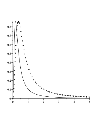
Figure 1: $H^{2}$, in terms of cosmic time for $w={1}(line)$, and $w=0$ (points)

The bounce is assumed to occur at $t=0$ and we have set $\rho_{c}\approx 0.41$, obtained by the Immirzi factor $\gamma\approx 0.24$ derived by studying the black hole entropy in loop Quantum Gravity in [9]. As it is illustrated in this figure, after the bounce at $t=0$, we have a super-inflation phase where $H$ is increasing. After $\dot{H}=0$, normal inflation phase begins. The super-inflation lasts longer for smaller $w$.

Obtaining an exact analytical solution for (4), and (6) is not generally possible. Indeed, (5) can not be easily integrated to give an analytic expression for $\rho(t)$ (note that only two of the equations (4), (5), and (6) are independent) but, as we have seen, choosing a constant EoS parameter facilitates the analysis.

To generalize the discussion to no constant EoS parameters, in the following we present a scalar field solution for the inflaton with power law potential which crosses $\dot{H}=0$ line, during its slow roll evolution. In general relativity, the slow roll model can only describe the inflation phase but here, as we will show, the super-inflation can occur also in the slow roll regime.

2.1 Slow roll scalar field solution crossing $\dot{H}=0$ line

In this part we assume that the inflaton is a slow-roll scalar field with a power law potential. We seek for solutions of Friedmann equations with differentiable Hubble parameter at transition time which as before we denote by $t_{0}$. We present a series which crosses $\dot{H}=0$ line, and show that by choosing appropriate parameters it satisfies the Friedmann equations.

The energy density of the scalar field is

$$\rho={1\over 2}\dot{\phi}^{2}+V(\phi)$$ (12)

where $V(\phi)$ is the potential and the pressure is given by

$$P={1\over 2}\dot{\phi}^{2}-V(\phi).$$ (13)

In the neighborhood of $t=t_{0}$, we present the differentiable Hubble parameter as [14]

$$H(t)=h_{0}+h_{1}(t-t_{0})^{p}+\mathcal{O}\left((t-t_{0})^{p+1}\right),$$ (14)

where $h_{0}$ is the value of the Hubble parameter and $p$ is the order of the first non zero time derivative of $H$ at $t=t_{0}$. If a negative $h_{1}={1\over p!}{d^{p}H\over dt^{p}}(t_{0})$ and an even integer number $p$ are found such that (14) satisfies the modified Friedmann equations, then this solution describes the transition from super-inflation to inflation, because for $t\leq t_{0}$ we have $\dot{H}\geq 0$ while for $t\geq t_{0}$ we have $\dot{H}\leq 0$. The differentiability of the Hubble parameter at transition time implies that the energy density and the pressure are well defined (see (4 and (6)).

To justify our ansatz (14), we show that it satisfies (5) and (6) consistently (note that (4) can be derived from (5) and (6)). The continuity equation for the scalar field reads

$$\ddot{\phi}+3H\dot{\phi}+V^{\prime}(\phi)=0,$$ (15)

where $V^{\prime}(\phi)={dV(\phi)\over d\phi}$. Substituting (14) into (15), with the assumption $\ddot{\phi}\ll 3H\dot{\phi}$, yields

$$3\left(h_{0}+h_{1}(t-t_{0})^{p}+\mathcal{O}\left((t-t_{0})^{p+1}\right)\right)\dot{\phi}+V^{\prime}(\phi)=0,$$ (16)

whose the solution for the power law potential

$$V(\phi)=v_{1}\phi^{n},$$ (17)

where $v_{1}$ is a real number and $n$ is an integer, is given by

$$\phi=\left({n(n-2)v_{1}(t-t_{0})\Phi(-{{(t-t_{0})^{p}h_{1}\over h_{0}}},1,{1\over p})\over 3h_{0}p}+c_{1}\right)^{1\over 2-n}.$$ (18)

$c_{1}$ is determined by

$$c_{1}=\phi^{2-n}(t_{0}),$$ (19)

and $\Phi$ is the Lerchphi function

$$\Phi(x,a,b)=\sum_{n=0}^{\infty}{x^{n}\over(b+n)^{a}}.$$ (20)

For quadratic potential,

$$V(\phi)={1\over 2}m^{2}\phi^{2},$$ (21)

we obtain

$$\phi=\phi(t_{0})\exp\left[{-m^{2}(t-t_{0})\Phi\left(-{(t-t_{0})^{p}h_{1}\over h_{0}},1,{1\over p}\right)\over 3h_{0}p}\right].$$ (22)

The slowly varying condition $\ddot{\phi}\ll 3H\dot{\phi}$, used to obtain the above solution, is satisfied when

$$\left|{n(n-1)v_{1}\over 9h_{0}^{2}}\phi^{n-2}(t_{0})\right|\ll 1,$$ (23)

which for quadratic potential gives $m^{2}\ll h_{0}^{2}$, leading to

$$m^{2}\ll\rho_{c}.$$ (24)

If we rewrite (23) as $\left|{d^{2}V\over d\phi^{2}}\right|\ll h_{0}^{2}$, in our slow roll regime, we deduce that the potential must satisfy $\left|{d^{2}V\over d\phi^{2}}\right|\ll V$, implying that the potential must be flat enough. Combining (23) with

$$v_{1}\phi^{n}(t_{0})\simeq{\rho_{c}\over 2}$$ (25)

(which means that in the slow roll approximation the main part of the energy density is coming from the potential), yields

$$\left|{n(n-1)\over 12\pi}\right|\ll\phi^{2}(t_{0}).$$ (26)

So the value of the scalar field at transition time must be large in this approximation.

By inserting (18) into the Friedmann equation

$$\dot{H}=-4\pi\dot{\phi}^{2}\left(1-{2\rho\over\rho_{c}}\right),$$ (27)

we arrive at

$$\dot{H}=-{8\pi\over 27\rho_{c}}\left({n^{2}v_{1}^{2}\phi^{2(n-1)}(t_{0})\over h_{0}^{3}}\right)\left({n^{3}(n-1)v_{1}^{3}\phi^{3n-4}(t_{0})\over 9h_{0}^{2}}+n^{2}v_{1}^{2}\phi^{2(n-1)}(t_{0})\right)$$

$$\times(t-t_{0})+\mathcal{O}\left((t-t_{0})^{2}\right)$$ (28)

So (14) satisfies Friedmann equation provided that

$$h_{1} = -{4\pi\over 27\rho_{c}}\left({n^{2}v_{1}^{2}\phi^{2(n-1)}(t_{0})\over h_{0}^{3}}\right)\left({n^{3}(n-1)v_{1}^{3}\phi^{3n-4}(t_{0})\over 9h_{0}^{2}}+n^{2}v_{1}^{2}\phi^{2(n-1)}(t_{0})\right),$$

$$p = 2.$$ (29)

Applying the slow roll condition (23) to (2.1), we obtain

$$h_{1}\simeq-{4\pi\over 27}{n^{4}v_{1}^{4}\left(\phi^{4}(t_{0})\right)^{n-1}\over h_{0}^{3}\rho_{c}},$$ (30)

which determines the transition rate. As $h_{1}<0$, our series solution

$$H \simeq \sqrt{{2\pi\over 3}\rho_{c}}-\sqrt{2\over 27\pi}{n^{4}v_{1}^{4}\phi^{4(n-1)}(t_{0})\over\rho_{c}^{5\over 2}}(t-t_{0})^{2}+\mathcal{O}\left((t-t_{0})^{3}\right)$$

$$\rho \simeq {\rho_{c}\over 2}-{n^{2}v_{1}^{2}\phi^{2(n-1)}(t_{0})\over\sqrt{6\pi\rho_{c}}}(t-t_{0})+\mathcal{O}\left((t-t_{0})^{2}\right),$$ (31)

where $\phi(0)$ is determined by (25), describes a transition from super-inflation to inflation at $t=t_{0}$. Note that the first term in the series solution of $H$ is the value of $H$ at the transition time, i.e. when $\rho={\rho_{c}\over 2}$. As a summary, we conclude that crossing the super-inflation-inflation divide line is, in principle, possible during a slow roll evolution of a scalar field with power law potential, and the approximate solution to Friedmann equations, in this region, is given by (2.1).

Compatibility of the slow roll scalar field model(with the power law potential (21))with observations was studied in [13]. In [13] WMAP7 [15] data were used to obtain some estimation about the value of the scalar field and its mass in the slow roll regime:

$$\phi(t_{*})=3.15m_{P},\,\,\,m=1.21\times 10^{-6}m_{P}.$$ (32)

$m_{P}$ is the Planck mass $m_{P}=\sqrt{\hbar c\over G}$. In the units adopted in this paper $m_{P}=1$. $t_{*}$ is some time in slow roll era, after super-inflation where the scale length $\lambda={1\over k}$ ($k=2\times 10^{-3}Mpc^{-1}$ is WMAP7 pivot scale) exited the Hubble radius. We can follow the procedure used in [13], to update the results (32) via Planck 2013 data [16]. In the scalar field model with square potential (21), the power spectrum of the scalar perturbations, $\mathcal{P}_{s}$, and the spectral index, $n_{s}$, are specified as

$$\mathcal{P}_{s} = {H^{2}\over\pi\epsilon}$$

$$n_{s} = 1-4\epsilon,$$ (33)

where

$$\epsilon = {1\over 16\pi}\left({V^{\prime}(\phi)\over V(\phi)}\right)^{2}$$ (34)

$$= {1\over 4\pi}{1\over\phi^{2}},$$

is one of the slow roll parameter. (2.1) must be computed at time $t_{*}$, where the scale length corresponding to the pivot scale $k=0.05Mpc^{-1}$ exited the Hubble Horizon. The Planck 2013 data imply (for $\%68$ CL or $1\sigma$ error)

$$\mathcal{P}_{s} = 10^{-9}\times(09616\pm 0.16)$$

$$n_{s} = 0.9616\pm 0.0094.$$ (35)

(2.1) together with (2.1) and (34) yield

$$4.71\times 10^{-11}<H^{2}(t_{*})<8.97\times 10^{-11}$$

$$6.66<\phi^{2}(t_{*})<10.98$$ (36)

and

$$1.01\times 10^{-6}<m<1.73\times 10^{-6}.$$ (37)

The estimated values for the inflaton mass in (37) and (32)are in agrement with our result (24). By noting that in the slow roll regime the main part of the energy is the potential energy, and also by bearing in mind that the energy decreases during the slow roll, we expect that the absolute value of $\phi$ decreases after the transition, $\left|\phi(t_{*})\right|<\left|\phi(t_{0})\right|$. Therefore (26) is also in agreement with (32) and (2.1).

3 Second and generalized second laws in loop quantum cosmology

The study of thermodynamic laws of cosmological horizons may provide us a mean to get more information about the solutions of (modified) Friedmann equations which describe the inflation and also the late time accelerated expansion of the universe. In this part we try to investigate the domain of validity of the generalized second law (GSL) (which asserts that the sum of the entropies of the horizon and the matter it encloses is a non decreasing function of cosmic time) in loop quantum cosmology for the solutions studied in the previous section, and also study the constraints that this law puts on these solutions.

The entropy of the apparent horizon $R_{h}$ in loop quantum gravity is given by [9]

$$S_{h}=\pi R_{h}^{2}+\pi\alpha\ln(\pi R_{h}^{2})+\beta,$$ (38)

where $\alpha\sim\mathcal{O}(1)$ and $\beta$ are real constants arisen from quantum corrections.

A natural choice for the cosmological horizon is the apparent horizon $R_{h}={1\over H}$ . Note that $R_{h}$ does not exists for $H=0$, but $R_{h}(H\neq 0)\in\mathbb{R}$. By adopting this choice we obtain

$$\dot{S_{h}}=-2\pi(1+\alpha H^{2}){\dot{H}\over H^{3}}.$$ (39)

Near $H=0$, $S_{h}$ is very large and $\dot{S_{h}}\approx-2\pi{\dot{H}\over H^{3}}$. So after the bounce, $S_{h}$ decreases very fast, reducing $S_{h}$ to smaller finite values. In the super accelerated expansion era, $H$ increases from $H=0$ at the bounce to $H=\sqrt{2\pi\rho_{c}\over 3}$ at the transition time, hence $S_{h}$ increases only for $-{3\over 2\pi\rho_{c}}<\alpha<0$, and when $(1+\alpha H^{2})<0$. After the transition, we have $\dot{H}<0$, and $\dot{S_{h}}>0$ is valid for $(1+\alpha H^{2})>0$.

To study the GSL, we must also consider the contribution of matter, which satisfies weak energy condition $\rho>0$, $P+\rho\geq 0$, to entropy. We use the first law of thermodynamics

$$dE=TdS_{in}-PdV,$$ (40)

to obtain

$$(P+\rho)dV+Vd\rho=TdS_{in}.$$ (41)

$T>0$ is the temperature and $S_{in}$ is the entropy of the matter inside the horizon. (42) and (5) result in

$$\dot{S_{in}}=-4\pi{(P+\rho)\over TH^{2}}(1+{{\dot{H}}\over H^{2}}).$$ (42)

During the inflation, $1+{{\dot{H}}\over H^{2}}>0$, therefore $\dot{S_{in}}<0$. After the inflation $S_{in}$ decreases.

By adding (42) to (39), we find that GSL is valid whenever

$$\dot{S}_{tot}=-2\pi(1+\alpha H^{2}){\dot{H}\over H^{3}}-4\pi{P+\rho\over TH^{2}}(1+{\dot{H}\over H^{2}})\geq 0.$$ (43)

Provided that the weak energy condition is valid, immediately after the bounce $S_{tot}$ quickly decreases. Afterward, the energy density decreases and the system approaches to the transition time. In the accelerated expansion era ($\dot{H}+H^{2}>0$), validity of GSL requires

$$\dot{H}(1+\alpha H^{2})<0,\,\,\,for\dot{H}>0,$$ (44)

and

$$\dot{H}(1+\alpha H^{2})<0,\,\,\,for\dot{H}<0.$$ (45)

By comparing (44) and (45), and assuming that $H$ is continuous at transition time, the value of $\alpha$ is fixed as

$$\alpha=-{1\over H^{2}(t_{0})}=-{3\over 2\pi\rho_{c}}\approx-1.16.$$ (46)

But this is not the whole history: In the super accelerated expansion epoch, $H$ increases until it reaches its maximum value $H=\sqrt{{2\pi\rho_{c}\over 3}}$ at transition time. But this result is in contradiction with (44) which implies $H(t<t_{0})>\sqrt{{2\pi\rho_{c}\over 3}}$. So we conclude that, besides a time interval after the bounce, GSL does not hold in the whole of a connected region comprising super-inflation, and ordinary inflation eras. Now let us have a closer look to the behavior of the system in the neighborhood of transition time $t_{0}$, when $\dot{S}_{tot}$ reduces to

$$\dot{S}_{tot}(t=t_{0})=-4\pi{P+\rho\over TH^{2}}.$$ (47)

The only way to save GSL in this region for ordinary matter (i.e. matter satisfying weak energy condition), is to have $P(t_{0})+\rho(t_{0})=0$. For the scalar field model, $P+\rho=\dot{\phi}^{2}\geq 0$. Based on the solutions derived in the previous section, the slow roll scalar field with power law potential (17) has the following behavior in neighborhood of $\dot{H}=0$ :

$$\dot{\phi}^{2}(t)={n^{2}v_{1}^{2}\phi^{2(n-1)}(t_{0})\over 6\pi\rho_{c}}-{2n^{3}(n-1)v_{1}^{3}\phi^{3n-4}(t_{0})\over\sqrt{216\pi^{3}}\rho_{c}^{3\over 2}}(t-t_{0})+\mathcal{O}((t-t_{0})^{2}).$$ (48)

But in the slow roll approximation, $V(\phi)\approx{\rho_{c}\over 2}$, then $\phi(t_{0})\neq 0$, and we have $\dot{S}_{tot}(t_{0})<0$. Therefore at $t_{0}$ and at least in the neighborhood of $t_{0}$ GSL is violated.

At the end of inflation,$t_{end}$, $\dot{H}+H^{2}=0$, and

$$\dot{S}_{tot}(t_{end})={2\pi\over H}(1+\alpha H^{2}).$$ (49)

Hence GSL violation is ceased at this time provided that $1+\alpha H^{2}>0$ which is always true for $\alpha>0$ (a positive value for $\alpha$ was proposed by [17]).

To be more quantitative and to get more insights about the GSL let us examine (43) using some of the solutions of Friedmann equations. To do this, we have to specify the matter temperature. This temperature is assumed to be equal to the horizon temperature which can be expressed in terms of surface gravity [18], $\kappa=-H\left(1+{\dot{H}\over 2H^{2}}\right)$, as

$$T=\left|{\kappa_{H}\over 2\pi}\right|=\left|{H\over 2\pi}\left(1+{\dot{H}\over 2H^{2}}\right)\right|.$$ (50)

So GSL states

$$\dot{S}_{tot}=2\pi{\dot{H}\over H^{3}}\left[-(1+\alpha H^{2})+\left({H^{2}+\dot{H}\over 2H^{2}+\dot{H}}\right)\left({2\rho_{c}\over\rho_{c}-2\rho}\right)\right]\geq 0.$$ (51)

Hence GSL holds whenever the above inequality is satisfied.

For a barotropic fluid with constant $w>0$, and by considering $\rho<\rho_{c}$, one can show that (51) reduces to

$$\left(1-2x\right)\left[-1-\alpha_{c}x(1-x)+\left({2\over 1-2x}\right)\left({-3\Gamma(1-2x)+2(1-x)\over 4(1-x)-3\Gamma(1-2x)}\right)\right]\leq 0$$ (52)

where $\Gamma=w+1$, and $x:={\rho\over\rho_{c}}$, $\alpha_{c}:={8\pi\over 3}{\alpha\rho_{c}}$ are dimensionless parameters. According to our previous claim, when $x\to 1$, the GSL is obviously violated. The same occurs when $x=1/2$, independently of the values of the parameters $\alpha$ and $\Gamma>1$. for $x\to 0$ and $\alpha H^{2}\ll 1$, (51) reduces to $\pi{{\dot{H}}^{2}\over H^{3}}\geq 0$ which is true. This is the domain of classical theory of gravity far from the Planck era. In this era GSL holds. The inflation ends at $x={3\Gamma-2\over 6\Gamma-2}$. In this region $\alpha>0$ is a sufficient condition for validity of GSL.

In figure (2), $\dot{S_{tot}}$ is depicted for a barotropic fluid whose equation of state parameter is $w\approx 1$ (e.g. a massless scalar field). GSL holds only for $t>0.22$ where the inflation nearly ends. The transition time is $t_{0}=0.18$ (to get more intuition, note these numbers are in terms of the fundamental time unit, $\sqrt{\hbar G\over c^{5}}$)

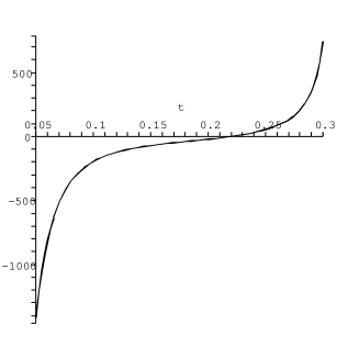
Figure 2: $\dot{S}_{tot}$ in terms of cosmic time for a single fluid with $w=1$ and $\alpha=-1.16$

So far, to elucidate our results, we have used the slow roll scalar field and barotropic fluids with constant EoS parameters. To get a more complete insight about the behavior of entropy for a nonconstant $w$, let us consider a scalar field with quadratic potential, (21), whose the kinetic energy is extremely dominated at the bounce [13]. One of the characteristics of this model is $f={\phi_{B}\over\phi_{max}}$, where $\phi_{max}^{2}={2\rho_{c}\over m^{2}}$ and $\phi_{B}$ is the value of the scalar field at the bounce. Therefore, $f^{2}={V(\phi)\over\rho_{c}}$ determines the contribution of the potential in the total energy density at the bounce. In [13], it was shown that for $f\geq 1.25\times 10^{-6}$ and $\phi_{B}>0$, this model is consistent with WMAP data. We take $\phi_{B}=1.1$, $\dot{\phi}_{B}=0.905$, $m=1.21\times 10^{-6}$ and $\alpha=-1.16$ which yield $f=1.4\times 10^{-6}$. As is depicted in fig.(3)) after the bounce and until the transition time $H$ is increasing, hence $\dot{H}+H^{2}>0$, thus this model is enable to describe the onset of inflation.

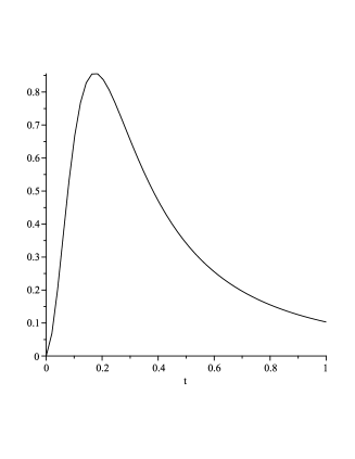
Figure 3: $H^{2}$ in terms of cosmic time for a scalar field model with quadratic potential and extreme domination of kinetic energy at the bounce

In fig.(4)), $\dot{S}$ is depicted in terms of the cosmic time . This figure shows that for $t<t\sim 0.2138$ GSL fails.

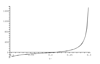
Figure 4: $\dot{S}$ in terms of cosmic time for a scalar field model with quadratic potential and extreme domination of kinetic energy at the bounce

4 Conclusion

We considered loop quantum cosmology, i.e. where the effective quantum corrections coming from loop quantum gravity cannot be neglected. We presented a slow roll scalar field solution with power law potential in terms of Lerchphi function and showed that this solution can describe the transition from the super-inflation to the inflation phase, provided that the value of the scalar field at transition time and the model parameters satisfy some conditions (see (23), (24) and (26)). It was shown that these conditions are consistent with Planck 2013 data. The thermodynamics second law and generalized second law (GSL) for the apparent horizon and for some previously proposed solutions were discussed. It was shown that if the matter respects the null energy condition, immediately after the bounce the (total) entropy decreases very fast from its huge values, but this decrease does not continue for a long time and after awhile the entropy begins to increase. It was shown that the GSL does not hold in the whole of a connected region extended from super-inflation to inflation era. Specially it was shown that for a scalar field this law is violated at transition time. As illustrations, we discussed the behavior of the entropy for an exactly solvable model (massless scalar field) where GSL is violated even after the transition time and holds (nearly) after the inflation ends. Afterwards using numerical method we depicted time derivative of the total entropy for scalar field model whose kinetic energy is extremely dominated at the bounce, and the violation of GSL in a finite time interval after the bounce was demonstrated.

So it seems that GSL does not hold near the bounce where the apparent horizon is very large, and at least, depending on the parameters of the model, this violation may continue until the end of inflation, as was illustrated through some examples. This violation is related to effective quantum effects and GSL continues to be true far from the Planck era. This may be related to the fact that in our computation we have ignored the contribution of the radiation energy density, generated by particle creation from the horizon [19]. Another possibility to alleviate this problem may be the adoption of another horizon such as the future event horizon [20]. Similar violation of GSL was also reported in a super-accelerated epoch in a phantom dominated universe or in modified theories of gravity in the literature [21].

References

- [1] A. Ashtekar, M. Bojowald, and J. Lewandowski, Adv. Theor. Math. Phys. 7, 233 (2003); Abhay Ashtekar, Gen. Rel. Grav. 41, 741 (2009); A. Ashtekar, Nuovo Cim. 122B, 135 (2007), arXiv:gr-qc/0702030.
- [2] E. J. Copeland, D. J. Mulryne, N. J. Nunes, and M. Shaeri, Phys. Rev. D 77, 023510 (2008).
- [3] G. M. Hossain, Class. Quant. Grav. 22, 2511 (2005); G. Calcagni and M. Cortes, Class. Quant. Grav. 24, 829 (2007); D. J. Mulryne and N. J. Nunes, Phys. Rev. D 74, 083507 (2006); Y. S. Piao and Y. Z. Zhang, Phys. Rev. D 70, 063513 (2004).
- [4] A. Linde, Particle Physics and Inflationary Cosmology (Harwood, Chur, Switzerland, 1990); A. Linde, Phys. Lett. B 129, 177 (1983).
- [5] A. Ashtekar, D. Sloan, Phys.Lett.B. 694, 108 (2010).
- [6] T. Jacobson, Phys. Rev. Lett. 75, 1260 (1995); R. G. Cai and S. P. Kim, J. High Energy Phys. 02, 050 (2005) 050; R. X. Miao, M. Li, and Y. G. Miao, JCAP 11, 033 (2011); Sh. F. Wu, B. Wang, G. H. Yang, and P. M. Zhang, Class. Quant. Grav. 25, 235018 (2008); K. Bamba, M. Jamil, D. Momeni, and R. Myrzakulov, arXiv:1202.6114v1 [physics.gen-ph]; V. Faraoni , arXiv:1005.2327v1 [gr-qc]; A. Ashtekar and E. Wilson-Ewing, Phys. Rev. D 78, 064047 (2008); K. Karami, A. Abdolmaleki, N. Sahraei, and S. Ghaffari, J. High Energy Phys. 1108, 150 (2011); H. M. Sadjadi, Phys. Scripta 05, 055006 (2011); H. M. Sadjadi and M. Jamil, Europhys. Lett 92, 69001 (2010); V. Faraoni, A. F. Z. Moreno, and R. Nandra, arXiv:1202.0719v1 [gr-qc]; K. Karami, M.S. Khaledian, and N. Abdollahi, arXiv:1201.4817v4 [physics.gen-ph]; H. M. Sadjadi , Europhys. Lett. 92, 50014 (2010); U. Debnath, Europhys. Lett. 94, 29001 (2011); V. Faraoni, Phys. Rev. D 80, 044013 (2009); M. Akbar, Int. J. Theor. Phys. 48, 2665 (2009); A. Das, S. Chattopadhyay, and U. Debnath, Found. Phys. 42, 266 ( 2011); Y. Zhang, Y. Gong, and Z. H. Zhu, Int. J. Mod. Phys. 20, 1505 (2011); H. M. Sadjadi and M. Honardoost, Phys. Lett. B 647, 231 (2007); Z. G. Liu and Y. S. Piao, arXiv:1203.4901 [gr-qc]; Y. S. Piao and E. Zhou, Phys. Rev. D 68, 083515 (2003).
- [7] P. C.W. Davies, Class. Quant. Grav. 4, L255 (1987); 5, 1349 (1988); D. Pavon, Class. Quant. Grav. 7, 487 (1990); R. Brustein, Phys. Rev. Lett. 84, 2072 (2000); T. M. Davis, P. C. W. Davies, and C. H. Lineweaver, Class. Quant. Grav. 20, 2753 (2003); K. Bamba, R. Myrzakulov, S. Nojiri, and S. D. Odintsov, arXiv:1202.4057v3 [physics.gen-ph]].
- [8] G. Izquierdo, D. Pavon, Phys. Lett. B 639, 1 (2006); M. D. Pollock and T. P. Singh, Class. Quant. Grav. 6, 901 (1989); S. Nojiri, S. D. Odintsov, Phys. Rev. D 72, 023003 (2005); H. Farajollahi, A. Salehi, and F. Tayebi, Can. J. Phys. 89, 915 (2011); S. Nojiri and S. D. Odintsov, Phys. Rev. D 70, 103522 (2004).
- [9] K. A. Meissner, Class. Quant. Grav. 21, 5245 (2004), A. Ghosh and P. Mitra, Phys. Rev. D 71, 027502 (2005).
- [10] D. Sloan, Loop Quantum Cosmology and the Early Universe , PhD Thesis, The Pennsylvania State University (2010); X. Zhang, Y. Ling, JCAP 08, 012 (2007), arXiv:0705.2656v2 [gr-qc].
- [11] E. W. Ewing, JCAP 1303, 026 (2013), arXiv:1211.6269 [gr-qc].
- [12] M. Bojowald, Living Rev. Rel. 8, 11 (2005); M. Bojowald, F. Hinterleitner, Phys. Rev. D 66 , 104003 (2002) 104003.
- [13] A. Ashtekar, and D. Sloan, Gen. Rel. Grav. 43, 3619 (2011).
- [14] H. M. Sadjadi and M. Alimohammadi, Phys. Rev. D 74, 043506 (2006).
- [15] E. Komatsu et al., Astrophys. J. Suppl. 192, 18 (2011), arXiv:1001.4538 [astro-ph.CO].
- [16] P. A. R. Ade et al., Planck 2013 results. XVI, arXiv: 1303.5076 [astro-ph] (2013); P. A. R. Ade et al., Planck 2013 results. I, arXiv: 1303.5062 [astro-ph) (2013).
- [17] S. Hod, Class. Quant. Grav. 21, L97 (2004).
- [18] R. G. Cai and S. P. Kim, J. High Energy Phys. 0502, 050 (2005).
- [19] S. K. Modak and D. Singleton, arXiv:1205.3404v1 [gr-qc].
- [20] A. Ashtekar and E. Wilson-Ewing, Phys. Rev. D 78, 064047 (2008).
- [21] G. Izquierdo and D. Pavon, Phys. Lett. B 633, 420 (2006); H. Mohseni Sadjadi, Phys. Rev. D 73, 063525 (2006); H. Mohseni Sadjadi, Europhys. Lett. 92, 50014 (2010).