Absolute detector calibration using twin beams

Abstract

A method for the determination of absolute quantum detection efficiency is suggested based on the measurement of photocount statistics of twin beams. The measured histograms of joint signal-idler photocount statistics allow to eliminate an additional noise superimposed on an ideal calibration field composed of only photon pairs. This makes the method superior above other approaches presently used. Twin beams are described using a paired variant of quantum superposition of signal and noise.

¹ RCPTM, Joint Laboratory of Optics of Palacký University and Institute of Physics of Academy of
Sciences of the Czech Republic, Faculty of Science, Palacký University, 17. listopadu 12,
77146 Olomouc, Czech Republic
² Institute of Physics of Academy of Sciences of the Czech Republic, Joint Laboratory of Optics of
Palacký University and Institute of Physics of Academy of Sciences of the Czech Republic,
17. listopadu 12, 772 07 Olomouc, Czech Republic
^∗Corresponding author: perinaj@prfnw.upol.cz

270.5570,190.4410,270.5290

The first suggestions to use photon pairs in absolute detector calibration have occurred soon after the experimental evidence of emission of photons in pairs in the process of spontaneous parametric down-conversion had been given [1]. The suggested method is based on the fact that both photons are created in the nonlinear process simultaneously. Provided that one (signal) photon is detected at its (signal) detector, we know for sure in the ideal case that the second photon exists in the beam [2]. Thus it impinges on a (idler) detector that is calibrated with probability one. Many repetitions of the experiment then provide the required absolute quantum detection efficiency (QDE) [3]. Following this simple scheme, absolute QDE $\eta_{i}$ of an idler detector is reached along the formula $\eta_{i}=\langle m_{s}m_{i}\rangle/\langle m_{s}\rangle$, where $\langle m_{s}m_{i}\rangle$ gives the number of coincidence counts at both detectors and $\langle m_{s}\rangle$ determines the number of signal-detector single counts. Weak photon fields having only a small fraction of a photon in a detection window on average are needed in this approach. The method automatically gives also QDE of the signal detector. It can be used for the calibration of both analog and photon-counting detectors with the precision comparable to other metrology methods exploiting thermal and semiconductor detectors [4].

The presented method, however, requires as ’the probe’ a weak field composed only of photon pairs. It is unable to cope with any additional noise in the form of un-paired single photons superimposed on the paired field. A simple analysis shows that the presence of additional single-photon noise counts $\langle m_{i}\rangle_{\rm noise}$ modifies the formula for QDE $\eta_{i}$; $\eta_{i}=\langle m_{s}m_{i}\rangle/\langle m_{s}\rangle-\langle m_{i}\rangle_{\rm noise}$. However, if single-photon noise is present in both fields, we cannot partition it from the paired part of the probe field. The improved formula QDE $\eta_{i}$ is thus not useful. Single-photon noise can only be eliminated as much as possible using a careful experimental arrangement.

Despite this drawback, the method has been generalized to include also stronger photon-pair fields [5] in which both pump-field intensity fluctuations and transverse correlations of photons in a pair play an important role. If the ratio of signal and idler QDEs is known and only a paired field is assumed, a simple relation between QDE and noise-reduction factor (quantifying sub-shot-noise photon correlations) can be revealed [5].

As we show in this letter, additional single-photon noise in the probe field can be eliminated considering photon-number resolving detectors like intensified CCD (iCCD) cameras [6, 7], array detectors [8] or electron-multiplied CCD (EMCCD) cameras [9]. This then allows to determine both signal and idler QDEs with, in principle, no precision limitations. The method is based on the measurement of joint signal-idler photocount distribution (JPCD) [10]. In detail, the experimental JPCD is fitted assuming a special form of the probe field derived in the framework of superposition of signal and noise applied to paired fields [11, 12]. This fitting uses both first and second photocount moments and minimizes declinations from the experimental photocount histogram [13]. This approach provides signal and idler QDEs, together with parameters of the noisy single-photon signal and idler fields giving a detailed detection characterization [14].

We demonstrate the general method by considering the measurement performed by an iCCD camera Andor. Multi-mode twin beams at the wavelength around 560 nm filtered by spectrally rectangular 14-nm wide (FWHM) interference filter have been generated by the pulsed third harmonics of a Ti:sapphire laser tuned at 840 nm in a non-collinear type-I interaction in a 5-mm long BaB₂O₄ crystal (for details, see [7]). Whereas the signal field has been directly sent to the photocathode of the camera, the idler field has been reflected on a dielectric mirror (reflectivity 99.2%) first and then impinged on a different area of the photocathode. This causes asymmetry in the signal ($\eta_{s}$) and idler ($\eta_{i}$) QDEs. Using pulsed pumping and repeating the measurement $\sim 10^{5}$ times, we have arrived at histogram $f(c_{s},c_{i})$ giving the number of measurements with the registered $c_{s}$ signal and $c_{i}$ idler photocounts. In the experiment, also the level of dark counts has to be monitored in order to allow for subtracting this additional, but independently quantified, noise.

A suitable choice of a general six-parameter form of the joint signal-idler photon-number distribution (JPND) together with appropriate values of signal ($\eta_{s}$) and idler ($\eta_{i}$) QDEs lies in the heart of the method. However, according to the theory of measurement, only values of the first and second moments of measured quantities are reliably determined after a reasonable number of measurement repetitions. Including the five measured values of the first and second moments, three free parameters remain in the considered eight-parameter problem. Our investigations have shown that the values of remaining three parameters are successfully revealed requiring the best fitting of the theoretical JPND to the experimental JPCD.

In the first step, we determine the first ($\langle c_{s}\rangle$, $\langle c_{i}\rangle$) and second ($\langle c_{s}^{2}\rangle$, $\langle c_{s}c_{i}\rangle$, $\langle c_{i}^{2}\rangle$) moments of the measured numbers of photocounts. Knowing the first ($\langle d\rangle$) and second ($\langle d^{2}\rangle$) moments of the dark-count distribution, its contribution to the measured photocount moments can be eliminated and moments of detected photoelectrons can be, step by step, found ($a=s,i$):

$$\langle m_{a}\rangle = \langle c_{a}\rangle-\langle d_{a}\rangle,$$

$$\langle m_{a}^{2}\rangle = \langle c_{a}^{2}\rangle-2\langle m_{a}\rangle\langle d_{a}\rangle-\langle d_{a}^{2}\rangle,$$ (1)

$$\langle m_{s}m_{i}\rangle = \langle c_{s}c_{i}\rangle-\langle m_{s}\rangle\langle d_{i}\rangle-\langle m_{i}\rangle\langle d_{s}\rangle-\langle d_{s}d_{i}\rangle.$$

On the other hand, the probe photon field ’in front of a detector’ can be considered as composed of three independent parts: pairs, signal noisy photons and idler noisy photons. They can be characterized by their numbers $M_{p}$, $M_{s}$, and $M_{i}$ of equally-populated modes and mean photon numbers $b_{p}$, $b_{s}$, and $b_{i}$ per mode, respectively. The first and second photon-number moments of these fields can be expressed as ($a=p,s,i$):

$$\langle n_{a}\rangle=M_{a}b_{a},\hskip 14.22636pt\langle(\Delta n_{a})^{2}\rangle=M_{a}b_{a}(1+b_{a}).$$ (2)

QDEs $\eta_{s}$ and $\eta_{i}$ provide the bridge between the ’theoretical’ photon-number moments and experimental photoelectron moments. Quantum detection theory [15] gives us ($a=s,i$):

$$\eta_{a}\left[\langle n_{p}\rangle+\langle n_{a}\rangle\right] = \langle m_{a}\rangle,$$

$$\eta_{a}^{2}\Biggl{[}\langle(\Delta n_{p})^{2}\rangle+\langle(\Delta n_{a})^{2}\rangle+\frac{1-\eta_{a}}{\eta_{a}}\left(\langle n_{p}\rangle+\langle n_{a}\rangle\right)\Biggr{]}$$

$$= \langle(\Delta m_{a})^{2}\rangle,$$

$$\langle(\Delta n_{p})^{2}\rangle = {\langle\Delta m_{s}\Delta m_{i}\rangle}/({\eta_{s}\eta_{i}}).$$

If QDEs $\eta_{s}$ and $\eta_{i}$ were known, Eq. (Absolute detector calibration using twin beams) would give five constraints for the determination of six parameters $M_{a}$ and $b_{a}$. This represents a serious problem arising from two points: (1) Only the first and second photoelectron moments are experimentally available with sufficient precision and (2) The probe photon field is non-classical due to its predominantly paired character that enforces the use of at least six independent parameters in its realistic description. The solution of Eq. (Absolute detector calibration using twin beams) can be expressed as a one-parameter system conveniently parameterized by the mean photon-pair number $\langle n_{p}\rangle$ ($a=s,i$):

$$\langle n_{a}\rangle = {\langle m_{a}\rangle}/{\eta_{a}}-\langle n_{p}\rangle,$$

$$\langle(\Delta n_{a})^{2}\rangle = \frac{\langle(\Delta m_{a})^{2}\rangle}{\eta_{a}^{2}}-\frac{\langle\Delta m_{s}\Delta m_{i}\rangle}{\eta_{s}\eta_{i}}-\frac{1-\eta_{a}}{\eta_{a}^{2}}\langle m_{a}\rangle,$$

$$\langle(\Delta n_{p})^{2}\rangle = {\langle\Delta m_{s}\Delta m_{i}\rangle}/(\eta_{s}\eta_{i}).$$ (4)

However, also QDEs $\eta_{s}$ and $\eta_{i}$ are not known. As the third and higher photoelectron moments cannot be reliably used for the chosen number of measurement repetitions [16], we suggest to minimize the declinations of experimental ($f$) and theoretical ($p_{c}$) photocount distributions. A JPCD $p_{c}$ can be derived from a JPND $p$ provided that the detection process is characterized. The JPND $p$ of a field composed of pair, signal, and idler components can naturally be written as a convolution of three Mandel-Rice distributions [15]:

$$p(n_{s},n_{i}) = \sum_{n=0}^{{\rm min}[n_{s},n_{i}]}p(n_{s}-n;M_{s},b_{s})$$ (5)

$$\mbox{}\times p(n_{i}-n;M_{i},b_{i})p(n;M_{p},b_{p});$$

$p(n;M,b)=\Gamma(n+M)/[n!\,\Gamma(M)]b^{n}/(1+b)^{n+M}$. Following Eq. (2), numbers $M_{a}$ of modes and mean photon-numbers $b_{a}$ per mode can be derived from the first and second photon moments occurring in Eq. (4) as follows ($a=p,s,i$):

$$b_{a}=\frac{\langle(\Delta n_{a})^{2}\rangle}{\langle n_{a}\rangle}-1,\hskip 11.38109ptM_{a}=\frac{\langle n_{a}\rangle^{2}}{\langle(\Delta n_{a})^{2}\rangle-\langle n_{a}\rangle}.$$ (6)

A detailed theory appropriate for a detector with $N$ pixels, QDE $\eta$ and dark-count rate $D\equiv\langle d\rangle/N$ has been developed in [16] and provided the probabilities $T(c,n)$ of having $c$ photocounts out of a field with $n$ photons:

$$T_{a}(c,n) = \begin{pmatrix}N_{a}\cr c\end{pmatrix}(1-D_{a})^{N_{a}}(1-\eta_{a})^{n}(-1)^{c}$$ (7)

$$\times\sum_{l=0}^{c}\begin{pmatrix}c\cr l\end{pmatrix}\frac{(-1)^{l}}{(1-D_{a})^{l}}\left(1+\frac{l}{N_{a}}\frac{\eta_{a}}{1-\eta_{a}}\right)^{n},a=s,i.$$

Using the formulas in Eqs. (5) and (7) the JPCD $p_{c}$ can be expressed as:

$$p_{c}(c_{s},c_{i})=\sum_{n_{s},n_{i}=0}^{\infty}T_{s}(c_{s},n_{s})T_{i}(c_{i},n_{i})p(n_{s},n_{i}).$$ (8)

Finally, the appropriate values of QDEs $\eta_{s}$ and $\eta_{i}$ and mean photon-pair number $\langle n_{p}\rangle$ are obtained by minimizing the function ${\cal D}$ quantifying the declinations of JPCD $p_{c}$ and experimental histogram $f$:

$${\cal D}=\sqrt{\sum_{c_{s},c_{i}=0}^{\infty}\left[p_{c}(c_{s},c_{i})-f(c_{s},c_{i})\right]^{2}}.$$ (9)

To practically demonstrate the power of the method, we discuss a typical measurement described in Fig. 1. Active area of the used iCCD camera is composed of 128x128 independent pixels with equal QDEs obtained by hardware binning of the original 1 megapixel resolution. Processing the raw data eliminates spatial blurring of the detection spots. Signal and idler photons are captured in different areas of the photocathode. Some pixels in the photocathode are also reserved for monitoring the noise. However, not all noises can be quantified this way. For example, single photons arising from fluorescence in the nonlinear crystal are difficult to monitor. There also occur pump-intensity fluctuations that modify the photon-pair statistics. As an example, we analyze the measurement that has resulted in the following photoelectron moments after eliminating dark counts: $\langle m_{s}\rangle=2.411\pm 0.002$, $\langle m_{i}\rangle=2.353\pm 0.004$, $\langle(\Delta m_{s})^{2}\rangle=2.489\pm 0.003$, $\langle(\Delta m_{i})^{2}\rangle=2.449\pm 0.005$, and $\langle\Delta m_{s}\Delta m_{i}\rangle=0.597\pm 0.003$. Applying the usual simplified method for the determination of QDE [neglecting noises in (Absolute detector calibration using twin beams) and assuming $\langle(\Delta n_{p})^{2}\rangle=\langle n_{p}\rangle$], we arrive at the values $\eta_{s}=\langle\Delta m_{s}\Delta m_{i}\rangle/\langle m_{i}\rangle=0.254\pm 0.001$ and $\eta_{i}=\langle\Delta m_{s}\Delta m_{i}\rangle/\langle m_{s}\rangle=0.248\pm 0.001$. For comparison, covariance of the measured signal and idler photocounts was $0.238\pm 0.001$ [5].

On the other hand and analyzing the data along the developed method, we obtain the graph of minimum declinations ${\cal D}$ depending on QDEs $\eta_{s}$ and $\eta_{i}$ as shown in Fig. 1.

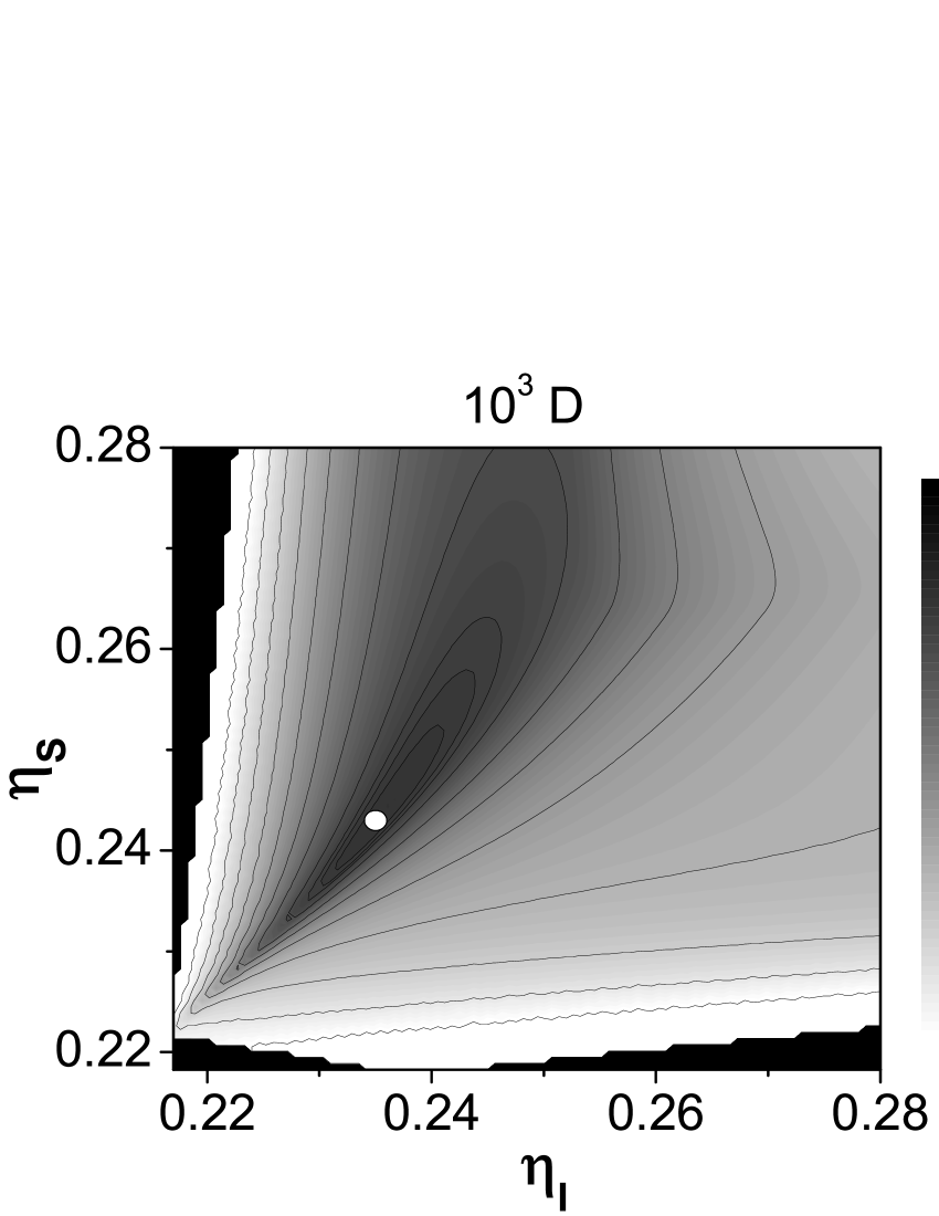
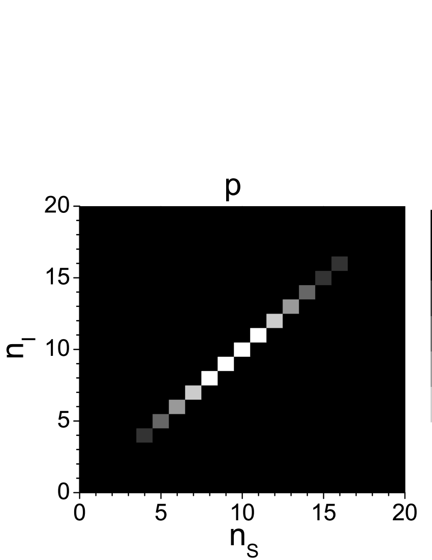
Figure 1: Minimum of declinations ${\cal D}$ determined over the allowed values of $\langle n_{p}\rangle$ depending on QDEs $\eta_{s}$ and $\eta_{i}$. In black areas close to $\eta_{s}$ and $\eta_{i}$ axes, Eqs. (Absolute detector calibration using twin beams) have no solution. For optimum values of QDEs $\eta_{s}=0.243$ and $\eta_{i}=0.235$, JPND $p(n_{s},n_{i})$ is shown.

The plotted minimum values of declinations ${\cal D}$ are found after scanning over the mean photon-pair number $\langle n_{p}\rangle$. The minimum value of declinations ${\cal D}$ has occured for QDEs $\eta_{s}=0.243\pm 0.001$ and $\eta_{i}=0.235\pm 0.001$. Whereas efficiency $\eta_{s}$ gives directly QDE of the camera, efficiency $\eta_{i}$ encompasses also reflectivity of the mirror placed in the path of the idler beam in perfect agreement with its independently measured value. The comparison with the values written above shows that partitioning the noisy parts of the probe field results in lower values of QDEs. The method has also provided the complete characteristics of the probe field with 1% relative error: $b_{p}=0.058$, $M_{p}=170$, $b_{s}=33.2$, $M_{s}=0.0007$, $b_{i}=10.6$, and $M_{i}=0.0101$. Thus, the probe field has contained on average 9.91 pairs, 0.02 signal noise photons and 0.11 idler noise photons. Despite the fact that the probe field has been nearly-exclusively composed of photon pairs (for the JPND, see Fig. 1), the effect of noise on the values of QDEs cannot be neglected. It holds that the larger the mean photon-pair number $\langle n_{p}\rangle$ the closer the values of QDEs obtained with the standard and the developed methods.

In conclusion, we have developed a method for precise determination of absolute detector efficiency of any photon-number resolving detector. The method allows to partition noise from the probe predominantly paired field thus providing, in principle, the precision in detector calibration limited only by the number of measurement repetitions. The improved precision and the possibility to use noisier probe fields make the method superior above other methods developed so far.

Support by projects P205/12/0382 of GA ČR and COST OC 09026 and CZ.1.05/2.1.00/03.0058 of the Ministry of Education of the Czech Republic is acknowledged. J.P.Jr. thanks J. Peřina for discussions.

References

- [1] D. C. Burnham and D. L. Weinberg, Phys. Rev. Lett. 25, 84 (1970).
- [2] A. A. Malygin, A. N. Penin, and A. V. Sergienko, Pisma Zh. Eksp. Teor. Fiz. 33, 493 (1981).
- [3] A. Migdall, Physics Today 52, 41 (1999).
- [4] G. Brida, M. Genovese, I. Ruo-Berchera, M. Chekhova, and A. Penin, J. Opt. Soc. Am. B 23, 2185 (2006).
- [5] G. Brida, I. P. Degiovanni, M. Genovese, M. L. Rastello, and I. R. Berchera, Opt. Express 18, 20572 (2010).
- [6] O. Haderka, J. Peřina Jr., M. Hamar, and J. Peřina, Phys. Rev. A 71, 033815 (2005).
- [7] M. Hamar, J. Peřina Jr., O. Haderka, and V. Michálek, Phys. Rev. A 81, 043827 (2010).
- [8] I. Afek, A. Natan, O. Ambar, and Y. Silberberg, Phys. Rev. A 79, 043830 (2009).
- [9] L. Zhang, L. Neves, J. S. Lundeen, and I. A. Walmsley, J. Phys. B: At. Mol. Opt. Phys. 42, 114011 (2009).
- [10] J. Peřina, J. Křepelka, J. Peřina Jr., M. Bondani, A. Allevi, and A. Andreoni, Phys. Rev. A 76, 043806 (2007).
- [11] J. Peřina and J. Křepelka, J. Opt. B: Quant. Semiclass. Opt. 7, 246 (2005).
- [12] J. Peřina and J. Křepelka, Opt. Commun. 265, 632 (2006).
- [13] A. P. Worsley, H. B. Coldenstrodt-Ronge, J. S. Lundeen, P. J. Mosley, B. J. Smith, G. Puentes, N. Thomas-Peter, and I. A. Walmsley, Opt. Express 17, 4397 (2009).
- [14] V. D’Auria, N. Lee, T. Amri, C. Fabre, and J. Laurat, Phys. Rev. Lett. 107, 050504 (2011).
- [15] J. Peřina, Quantum Statistics of Linear and Nonlinear Optical Phenomena (Kluwer, Dordrecht, 1991).
- [16] J. Peřina Jr., O. Haderka, M. Hamar, and V. Michálek, Phys. Rev. A 85, 023816 (2012).