Asymmetric chiral alignment in magnetized plasma turbulence

Abstract

Multi species turbulence in inhomogeneous magnetised plasmas is found to exhibit symmetry breaking in the dynamical alignment of a third species with the fluctuating electron density and vorticity with respect to the magnetic field direction and the species’ relative background gradients. The possibility of truly chiral aggregation of charged molecules in magnetized space plasma turbulence is discussed.

This is a preprint version of a manuscript accepted 10/2012 for publication in Physics of Plasmas.

I Introduction: drift wave turbulence

Drift wave turbulence Hor99 is composed of coupled nonlinear fluctuations of pressure $p$ and the electrostatic potential $\phi$ in an inhomogeneous plasma with a guiding magnetic field ${\bf B}$. The local electrostatic potential acts as a stream function for the dominant plasma flow with the drift velocity. The plasma is advected around the isocontours of a potential perturbation perpendicular to the magnetic field and forms a quasi two-dimensional vortex: an initial localized plasma density perturbation rapidly loses electrons along the magnetic field ${\bf B}$, leaving a positive electrostatic potential perturbation $\phi$ in its place. The associated electric field ${\bf E}=-\bm{\nabla}\phi$ is directed outward from the perturbation centre, and in combination with a magnetic field ${\bf B}$ causes an ”E-cross-B” vortex drift motion of the whole plasma along isocontours of the potential with a velocity ${\bf v}_{E}={\bf E}\times{\bf B}/B^{2}$.

This gyration averaged drift motion is a result of the combined electric and magnetic forces acting on a charged particle with small gyration radius compared to background scales Hor99 . In the presence of a background density (or pressure) gradient $\bm{\nabla}n$ the vortex propagates in the direction perpendicular to both $\bm{\nabla}n$ and ${\bf B}$. Drift waves become unstable if the electron density can not rapidly adapt to the electrostatic potential along the direction parallel to ${\bf B}$, which can be caused by interaction of the electrons with other particles or waves. Nonlinear coupling of drift waves results in a self-sustained fully developed turbulent state Has83 ; Sco90 .

The requirements for the occurrence of drift waves are ubiquitously met in inhomogeneous magnetized plasmas when the drift scale $\rho_{s}=\sqrt{(M_{i}T_{e})/(eB)}$ is much smaller than the background pressure gradient length $L_{p}=(\bm{\nabla}\ln p)^{-1}$, or equivalently, when the fluctuation frequency $\omega$ is much smaller than the ion gyration frequency $\omega_{ci}=eB/M_{i}$. Here $M_{i}$ is the ion mass, $T_{e}$ the electron temperature (in eV), $e$ the elementary charge, $B$ the magnetic field strength, and $p=n_{e}T_{e}$ the electron pressure.

Drift wave vortices are mainly excited in the size of a few drift scales $\rho_{s}$ and nonlinearly dually cascade to both smaller and larger scales. This perpendicular spatial scales of turbulent fluctuations are characteristically much smaller than any parallel fluctuation gradients and scales, so that wave vectors fulfill $k_{||}\ll k_{\perp}$.

Particle aggregation and transport in turbulence is a widely studied subject in fluid dynamics Pro99 . In turbulent plasmas the aggregation of charged particles is in addition influenced by static and dynamic electric and magnetic fields. For gyrofluid drift wave turbulence in inhomogeneous magnetized plasmas it has been observed by Scott Sco05 that the gyrocenter density of light positive trace ions (in addition to electrons and a main ion species) in three-species fusion plasma drift wave turbulence tend to dynamically align with the fluctuating electron density, so that fluctuation amplitudes of the electron and trace ion densities are spatiotemporally closely correlated. Priego et al. Pri05 have found that the particle density of inertial impurties in a fluid drift wave turbulence model is also closely correlated with the ExB flow vorticity.

The present analysis shows that the dynamical alignment in drift wave turbulence is not only sign selective with respect to the vorticity of trapping eddies, for any given trace species charge and background magnetic field direction, but also their large-scale background gradient.

The resulting asymmetric effects on transport and aggregation of charged particles is specifically discussed for application to space plasmas, in particular for cases of a nearly collisionless plasma with cold ions and low parallel electron resistivity, where the electrostatic potential closely follows changes in the electron density. It is shown that in this case drift wave turbulence constitutes a unique mechanism for truly chiral vortical aggregation of charged molecules in space environments with a background magnetic field and plasma density gradients.

This paper is organized as follows: in section II the cold-ion gyrofluid model equations for the present multi-species drift wave turbulence studies are introduced. Section III describes the numerical methods, and in section IV the computational results are presented. Section V discusses implications of the results for chiral particle aggregation in turbulent space plasmas, which poses a possible extraterrestrial physical mechanism for achieving enantiomeric excess in prebiotic molecular synthesis. The relation between the present gyrofluid model and the inertial fluid model by Priego et al. Pri05 is considered in the Appendix.

II Model: multi-species (cold ion) gyrofluid equations

Multi-species drift wave turbulence in the weakly collisional limit can be conveniently treated within a gyrofluid model. Here a strongly reduced variant of the gyrofluid electromagnetic model (“GEM”) by Scott Sco10 is adapted for numerical computation of three-species drift wave turbulence in a quasi-2D approximation in the electrostatic, isothermal, cold ion limit (neglecting finite Larmor radius effects) with a dissipative parallel coupling model.

The gyrocenter particle densities $n_{s}$ for (electron, main ion, and trace ion) species $s\in(e,i,z)$ are evolved by nonlinear advection equations

$$D_{t}n_{s}=(\partial_{t}+{\bf v}_{E}\cdot\bm{\nabla})n_{s}=\partial_{t}n_{s}+[\phi,n_{s}]=C_{s},$$ (1)

where all $C_{s}$ include hyperviscous dissipation terms $\nu_{4}\nabla^{4}n_{s}$ for numerical stability. The parallel gradient of the parallel fluid velocity components are for simplicity expressed by assuming a single parallel wave vector $k_{||}$ in the force balance equation along the magnetic field Has83 . Then $C_{e}$ in addition includes the coupling term $d(\phi-n_{e})$, where $d$ is the parallel coupling coefficient proportional to $k_{||}^{2}/\nu_{ei}$. For weakly dissipative plasmas $d$ is well larger than unity, but for practical purposes $d=2$ already sufficiently supports nearly adiabatic coupling between $n_{e}$ and $\phi$ while allowing reasonable time steps. The coupling can be regarded as non-adiabatic when $d<1$.

The electrostatic potential is here derived from the local (linear) polarization equation

$$\rho_{m}\nabla^{2}\phi=n_{e}-n_{i}-a_{z}n_{z},$$ (2)

where $\rho_{m}=1+a_{z}\mu_{z}$ with $a_{z}=Zn_{z}/n_{e}$ and $\mu_{z}=m_{z}/(Zm_{i})$. In the local model only the density perturbations are evolved in the advection equations, which then gain an additional background advection term $g_{s}\partial_{y}\phi$ with $g_{s}=(L_{\perp}/L_{ns})$ on the right hand side, where $L_{\perp}$ is a normalising perpendicular scale (here set identical to $L_{ne}$ so that $g_{e}=g_{i}=1$) and $y$ is the coordinate perpendicular to both the magnetic field and the background gradient directions. In the following only trace ions with $a_{z}\ll 1$ are considered, and the parameter $a_{z}=0.0001$ is going to be fixed, while other parameters are being varied.

The 2D isothermal gyrofluid model and its relation to (inertial) fluid models is briefly discussed in the Appendix.

III Method: numerical simulation and analysis

The numerical scheme for solution of the advection and polarization equations is described (for a similar ”Hasegawa Wakatani” type code where the ion density equation is replaced by a vorticity equation) in refs. Ken11 ; Shu11 .

The present computations use a $512\times 512$ grid corresponding to $(64\;\rho_{s})^{2}$ in units of the drift scale. This is a resolution well established for drift wave turbulence computations, resolving both the necessary small scales just below the gyro radius (or drift scale), and also allowing enough large scales for fully developed turbulent spectrum. The results converge for both higher resolution and same size in drift units, and for larger size with accordingly increased grid nodes.

The computations are initialized with quasi-turbulent random density fields and run until a saturated state is achieved. The resulting turbulent advection dynamics is restrained to the 2-dimensional plane perpendicular to the (local) magnetic field Ken08 . Statistical analysis is performed on spatial and temporal fluctuation data in this saturated state. The turbulence characteristics of drift wave systems (like power spectra, probability distributions, etc.) in general have been extensively discussed before, so that here the focus is on analysis of the correlation of the fluctuating density of the additional species with the other fluctuating fields.

IV Results: asymmetric dynamical alignment

In accordance with ref. Sco05 we also observe in our simulations that the gyrocenter density of a low-density massive trace ion species tends to dynamically align with the electron density $n_{e}$.

The anomalous diffusion, clustering and pinch of impurities in plasma edge turbulence has also been studied previously by Priego et al. Pri05 . In this paper the impurities were modeled as a passive fluid advected by the electric and polarization drifts, while the ambient plasma turbulence was modeled using the 2D Hasegawa-Wakatani model. As a consequence of compressibility it has there also been found that the density of inertial impurities correlates with the vorticity of the ExB velocity. Trace impurities were observed to cluster in vortices of a precise orientation determined by the charge of the impurity particles Pri05 .

The major difference to the present approach is that Priego et al. have considered only a constant impurity background (i.e. no impurity background gradient), but have in addition included additional nonlinear inertial effects through the impurity polarization drift. Linear inertial effects by polarization are already consistently included in the local gyrofluid model. The detailed correspondence between the two models is discussed in the Appendix.

For an initial homogeneous distribution of impurities with no background gradient ($g_{z}=0$) and vanishing (or constant) initial perturbation $n_{z}(t=0)=0$ the perturbed gyrocenter density $n_{z}(t)$ remains zero for all times, which directly follows from the evolution equation $D_{t}n_{z}=0$. The perturbed fluid particle impurity density $N_{z}$ is related to the cold impurity gyrocenter density by the transformation $N_{z}=n_{z}+\mu_{z}\Omega$ (see Appendix). As a result the perturbed fluid particle impurity density evolves according to $D_{t}N_{z}=\mu_{z}D_{t}\Omega$ and directly follows the vorticity, which has also been observed in fluid simulations by Priego et al. Pri05 . In the following the focus is on additional effects of a finite impurity background density gradient specified by $g_{z}$.

In the adiabatic (weakly collisional) limit the electrons can be assumed to follow a Boltzmann distribution with

$$(n_{0}+n_{e})=n_{0}\exp[e\phi/T_{e}]\approx n_{0}\;(1+e\phi/T_{e}),$$ (3)

so that (for given $T_{e}$ and $n_{0}$) a positive $n_{e}$ perturbation corresponds to a positive localized potential perturbation $\phi$. The ${\bf v}_{E}\sim(-\bm{\nabla}\phi\times{\bf B})$ drift motion of a plasma vortex around a localized $\phi$ perturbation possesses a vorticity

$${\bf\Omega}=\bm{\nabla}\times{\bf v}_{E}=({\bf B}/|B|)\nabla^{2}\phi,$$ (4)

related to the Laplacian of the electrostatic potential, and thus (depending on the sign of the fluctuating potential) a definite sense of rotation with respect to the background magnetic field ${\bf B}/|B|$.

In ref. Sco05 the absolute correlation $|r(n_{e},n_{z})|$ between the (gyrocenter) density perturbations of electrons $n_{e}$ and trace ions $n_{z}$ has been determined. Our present analysis in addition shows that under specific conditions a definite sign relation appears for the sample correlation coefficient

$$r(n_{e},n_{z})={{\sum(n_{e}-\overline{n}_{e})(n_{z}-\overline{n}_{z})}\over\sqrt{\sum(n_{e}-\overline{n}_{e})^{2}\sum(n_{z}-\overline{n}_{z})^{2}}},$$ (5)

where the sum $\sum$ is taken over all grid points of the computational domain, and the bar $\overline{n}_{s}$ denotes the domain average of the specific particle density.

In local computations with the present model, where the densities are split into a static spatially slowly varying background component $n_{0}$ with perpendicular gradient lengths $L_{n}=(\nabla\ln n_{0})^{-1}$ and a fluctuating part with small amplitudes $n$ (typically in the range of a few percent), the sign and value of $r(n_{e},n_{z})\approx\pm(0.90\pm 0.02)$ are observed to only depend on the relative sign but not the magnitude of the gradient lengths $L_{ne}$ and $L_{nz}$, for a given direction of the background magnetic field and fixed other parameters ($d=2$, $\mu_{z}=10$).

The result for $r(n_{e},n_{z})$ changes only marginally for most other parameter variations. In particular, the sign of the impurity charge $Z$ has no effect on the alignment property. Stronger adiabaticity leaves $r(d=10)\approx\pm(0.90\pm 0.02)$ largely unchanged, while a smaller (strongly non-adiabatic) dissipative coupling coefficient results in $r(d=0.01)\approx\pm(0.79\pm 0.02)$. In Fig. 1 the computed turbulent fields of vorticity (left figure) and a heavy (for example molecular) charged particle species density perturbation (right) in the 2D plane perpendicular to B are shown in a snapshot to be closely (negatively) spatially correlated for parameters $d=2$ (quasi-adiabatic) and $g_{z}=L_{\perp}/L_{nz}=+0.001$ (co-aligned background density gradients).

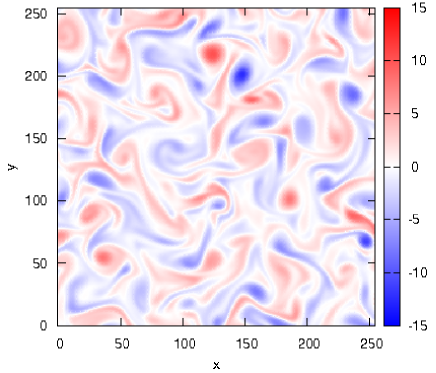
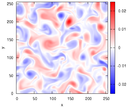
Figure 1: Left: Vorticity $\Omega(x,y)$; right: trace ion gyrocenter density perturbation $n_{z}(x,y)$. Normalized amplitudes are used and only a quarter of the complete computational domain is shown. $\Omega$ and $n_{z}$ here show close negative alignment for weak (quasi-adiabatic) coupling with $d=2$. The (co-aligned) impurity gradient length is here set to $L_{\perp}/L_{nz}=+0.001$.

Table 1: correlation coefficient $r(n_{e},n_{z})$
$g_{z}$ $d$ $r(n_{e},n_{z})$ $+0.001$ $2.00$ $+0.90\pm 0.01$ $+0.100$ $2.00$ $+0.90\pm 0.01$ $+1.000$ $2.00$ $+0.91\pm 0.01$ $-1.000$ $2.00$ $-0.90\pm 0.01$ $-0.100$ $2.00$ $-0.91\pm 0.01$ $-0.001$ $2.00$ $-0.90\pm 0.01$ $+0.001$ $10.0$ $+0.90\pm 0.02$ $+0.001$ $2.00$ $+0.90\pm 0.01$ $+0.001$ $1.00$ $+0.92\pm 0.01$ $+0.001$ $0.10$ $+0.87\pm 0.01$ $+0.001$ $0.01$ $+0.79\pm 0.02$

The observed sign-selective multi-species dynamical alignment effect is basically caused by the (linear) drive of density fluctuations $\partial_{t}n_{z}\sim g_{z}\partial_{y}\phi$ by this background advection term, where the potential $\phi$ is for each species just acting on the respective background gradients with length $L_{ns}$. The species gyrocenter densities are enhanced (positive partial time derivative) when the background advection is positive, and decreased when negative. Co-aligned background gradients of electrons and trace ions thus dynamically also imply co-alignment of the gyrocenter density perturbations. In case of adiabatic electrons this additionally implies negative alignment with vorticity, as can be seen in Fig. 1. For counter-aligned background density gradients the plot for $n_{z}(x,y)$ in Fig. 1 has exactly the same topology only with signs reversed, i.e. blue and red in the colour scale exchanged.

Strong non-adiabaticity ($d\ll 1$) only slightly reduces the electron-to-impurity density correlation coefficient $r(n_{e},n_{z})$ compared to adiabatic cases. Although the alignment between electron density and electrostatic potential is reduced for a non-adiabatic response, the alignment between the impurity gyrocenter density $n_{z}$ and vorticity $\Omega$ still remains.

The results for $r(n_{e},n_{z})$ as a function of the dissipative coupling parameter $d$ and (co- or counter-aligned) impurity gradient length $g_{z}=L_{\perp}/L_{nz}$ are summarized in Table 1.

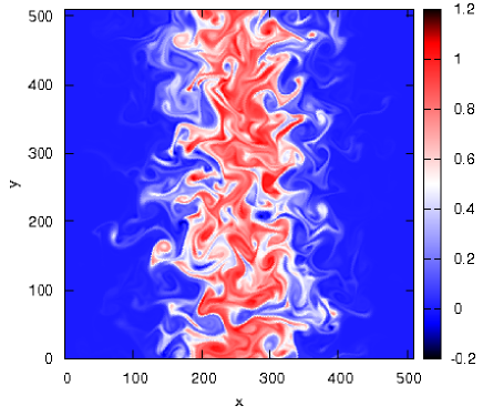
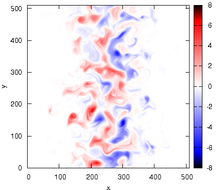
Figure 2: A Gaussian trace ion puff placed in the turbulent plasma is initially localized around the center of the $x$ domain (and constant in $y$). Left: impurity density $n_{z}(x,y)$. Right: the product function $\Omega(x,y)\cdot n_{z}(x,y)$ shows in comparison with the top figure that impurity density and vorticity are preferentially negatively aligned in the right half of the domain (where the initial density gradients are co-aligned) and positively aligned on the left.

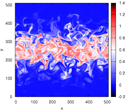
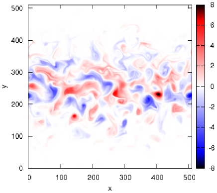
Figure 3: A Gaussian trace ion puff placed in the turbulent plasma is initially localized around the center of the $y$ domain (and constant in $x$). Left: impurity density $n_{z}(x,y)$. Right: the product function $\Omega(x,y)\cdot n_{z}(x,y)$ shows that in this case no preferential sign of alignment between impurity density and vorticity is found.

The situation is different if there is no background distribution of the trace ion species, but only a smaller localized cloud (diffusing over time) with an initial spatial extension in the same order of magnitude as the turbulence scales. Then the cloud can have global gradients of its density in all directions with respect to the background electron (and primary ion) gradient, and the signs of $r$ approximately can cancel to zero by integration over the computational domain, while the absolute correlation coefficient $|r|$ remains near unity.

The turbulent spreading of such a initially Gaussian trace ion puff (with zero background) strongly localized in $x$ or $y$ is shown in Figs. 2 and 3, respectively. In Fig. 2 a Gaussian trace ion puff placed in the turbulent plasma is initially localized around the center of the $x$ domain and constant in $y$. The product function $\Omega(x,y)\cdot n_{z}(x,y)$ shows (in the left part of the figure) in comparison with the impurity gyrocenter density $n_{z}(x,y)$ (right figure) that $n_{z}(x,y)$ and $\Omega(x,y)$ are preferentially negatively aligned in the right half of the domain, where the initial density gradients are co-aligned, and positively aligned on the left. This behaviour is in accordance with the previous result for a constant background gradient, as has been shown in Fig. 1 For the $x$-symmetric case in Fig. 3 no preferential sign of alignment between impurity gyrocenter density and vorticity is found.

Also this case the perturbed fluid particle density $N_{z}$ is still correlated with vorticity according to the relation $D_{t}N_{z}=\mu_{z}D_{t}\Omega$. The preceding discussion of the present results was funded within the gyrocenter density $n_{z}$ representation of the gyrofluid model. It remains to be clarified when the advection by the background gradient or the inertial contribution is the dominant factor that determines alignment of the fluid particle density $N_{z}=n_{z}+\mu_{z}\Omega$ with vorticity.

In Fig. 4 the correlation coefficient $r(\Omega,N_{z})$ is shown as a function of the impurity density gradient parameter $g_{n}$ at $d=2$ for $\mu_{z}=10$ (circles, bold solid line), $\mu_{z}=30$ (squares, thin dashed line) and $\mu_{z}=-10$ (diamonds, thin solid line). The alignment of perturbed impurity particle density with vorticity changes sign around $g_{n}\approx\mu_{z}/2$: for $g_{n}\ll\mu_{z}$ the alignment directly follows the vorticity with $r(\Omega,N_{z})\approx 1$, and for $g_{n}\gg\mu_{z}$ the alignment is reversed towards negative vorticity with $r(\Omega,N_{z})\approx-1$.

The computations have been repeated for a non-adiabatic parallel coupling coefficient $d=0.1$, for which the results remain very similar. The overall impression given by Fig. 4 does not change signficantly in this case, except for slight (order of per cent) differences within fluctuation averaging errors.

The sign of alignment is thus determined by the strength of the impurity gradient in relation to the mass-to-charge ratio of the impurities. For example, for singly positively charged heavy molecules (like typical space biomolecules) with $\mu_{z}\gg 1$ and small impurity gradient $g_{z}\approx 1$ the alignment is tendentially towards positive vorticity. For vanishing impurity gradient ($g_{z}=0$) the correlation $r(\Omega,N_{z})$ is always exactly $+1$ for positively charged impurities, and $-1$ for negative impurities.

Figure 4: Correlation coefficient $r(\Omega,N_{z})$ as a function of the impurity density parameter $g_{n}$ for $\mu_{z}=10$ (circles, bold solid line), $\mu_{z}=30$ (squares, thin dashed line) and $\mu_{z}=-10$ (diamonds, thin solid line): the alignment of impurity particle density with vorticity changes sign around $g_{n}\approx\mu_{z}/2$.

The basic conclusion is that for given background gradients and magnetic field direction the perturbed trace ion species gyrocenter density dynamically aligns with a definite sign of the electron density fluctuations, and thus of the electrostatic potential fluctations, and consequently of vorticity ${\bf\Omega}$: for example, an excess of trace ions aggregates within vortices of clockwise direction, and a deficit is found in vortices with anti-clockwise direction (or vice versa, depending on global parameters).

While, as usual in a fully developed turbulent state, vortices of both signs appear equally likely and evenly distributed over all turbulent scales, the trace particle aggregation on drift scales emerges with one prefered rotationality with respect to the background magnetic field and background particle gradients.

V Chiral molecular aggregation in drift wave turbulence

Finally, a possible relevance of the asymmetric alignment effect on molecular chemistry in a magnetized space plasma environment is suggested.

Homochirality of biomolecules – the fact that the essential chemical building blocks of life have a certain handedness while synthetic production leads to equal (racemic) distribution of left-handed and right-handed chiral structures – has ever since its discovery by Pasteur Pas48 posed a formidable puzzle Mas84 ; Lou02 . Pasteur already had unsuccessfully tried to identify physical causes for this biological symmetry breaking, for example by imposing chirality through fluid vortices in a centrifuge, and by exposing chemical solutions to a magnetic field Pas84 .

A number of theories and experiments on the origin of chirality have since been put forward, like effects of circularly polarized light on the molecular reactions Huc96 ; Bai98 ; Bow01 or a combination of magnetic field and non-polarized light Rik00 , or possible electroweak effects on quantum chemistry Ber01 . All of these mechanisms could be active in interplanetary and interstellar space, and would hint on an extraterrestrial origin of early fundamental biomolecules.

That chirality can in principle indeed be imposed by rotational forces has been confirmed experimentally for different situations Rib01 ; Mic12 , but what mechanism could invoke a specific directionality in turbulent (terrestrial or space) fluids or plasmas, where vortices of both senses of rotation generically occur mixed across all scales, has been left an open question. Here we argue that rotation asymmetric ion aggregation in drift vortices in magnetized space plasmas constitutes a mechanism for fostering a truly chiral environment for enantiomeric selective extraterrestrial formation of biomolecules.

The drift scaling conditions and possibilities for occurrence of drift wave turbulence are well fulfilled for a number of typical space plasma parameters and magnetic field strengths, like in (warm ionized) clouds in the interstellar medium How06 .

The background pressure or density gradient length of molecular ion species in the interstellar medium can take values across many orders of magnitude. While interstellar clouds range in size between a few and hundreds of parsecs (1 pc = $3.0857\cdot 10^{16}$ m) and thus have global gradient lengths of the same order, the local gradients can be set by macroscopic turbulence (resulting from large scale magnetohydrodynamic motion or by chaotic external drive through winds and jets) and vary widely, from observable scales of 100 pc down to 1000 km Gae11 .

Then again, the gradient of molecular ion density can also be set by a spatially varying degree of ionization, for example through inhomogeneous irradiation at the edge of molecular clouds. Magnetic field strengths in the interstellar medium can occur up to a few $\mu$G to mG, and temperatures range between 10 K in cold molecular clouds to 10000 K in warm ionized interstellar medium. The resulting drift (and vortex) scale $\rho_{s}$ is in the order between a few hundred meters and a few hundred kilometers.

Typical vortex life times are in the order between seconds and hours. The mean free path (parallel to a magnetic field) between particle collisions is in the order of 1000 km, so that the plasma is only weakly collisional. The drift ratio is in the maximum order of $\delta=\rho_{s}/L_{p}=0.1$ and smaller, thus well below unity.

The relative fluctuation amplitudes (compared to background values of the plasma density) in drift wave turbulence are typically in the order of the drift ratio and thus here in the range of a few percent or below. Compared to macroscopic flow-driven or magnetohydrodynamic (MHD) turbulence, drift wave turbulence is most effective on smaller scales, in the order of $\rho_{s}$, and with relatively small amplitude. Drift wave vortices in the size between a few hundred meters and hundreds of kilometers are thus expected to be present in most interstellar plasmas.

Next we consider, if such vortices truly can account for a chiral physical effect. Chiral synthesis usually requires a truly chiral influence Bar86 ; Bar12 : the parity transformation $(P:x,v\rightarrow-x,-v)$ has to result in a mirror asymmetric state that needs to be different from simply a time reversal $(T:t\rightarrow-t)$ plus a subsequent rotation by $\pi$. A purely 2D vortex can not exert a truly chiral influence, while 3D funnel-like fluid vortices in principle do. While a bulk rotation per se can not cause any direct polarizing effect on the reaction path for molecular synthesis Fer99 , particle aggregation on a supramolecular level in vortex motion has been experimentally shown to be able to lead to chiral selection Rib01 . To date it however remains unclear how chirality from a supramolecular aggregate (clusters or dust) could be transfered to single molecules Fer01 .

In the case of drift wave turbulence the parallel wave-like dynamics imposes a wave vector $k_{||}$ that under $P$ changes direction with respect to the vorticity ${\bf\Omega}$ and ${\bf B}$ (which themselves are pseudovectors and remain invariant under $P$), equivalently to a 3D vortex tube. Drift wave turbulence is thus truly chiral, although it characteristically appears quasi-two-dimensional. In case of a large-scale density gradient $\nabla_{||}n$ along ${\bf B}$ the (small) $k_{||}$ is given by this gradient length, otherwise it is determined by local fluctuations. Molecular ions are advected by the drift vortex motion, and are subjected to chiral aggregation onto neutral molecules, clusters or dust particles that are not participating in the plasma rotation.

If in addition (as to be rather expected in most cases) a trace ion background density gradient in the direction parallel to ${\bf B}$ is present, the resulting parallel wave vector $k_{||}$ prescribes in combination with vorticity ${\bf\Omega}$ a definite true chiral vortex effect. Chemical reactions in this system occur by collisions or aggregation of ions, that participate in the chiral vortex rotation, with neutral molecules or clusters of the quiescent (non rotating) background gas. The co- or counter alignment of ${\bf B}$ with ${\bf\Omega}$ can further act as chiral catalyst.

The chiral influence however changes sign in different sides or regions of the (large-scale) molecular cloud, when the relative direction of background particle gradient and magnetic field direction reverses. This implies that different regions of the interstellar medium favour different tendencies for chiral selective aggregation, and thus for a potential enantiomeric excess in molecular syntheses. The excess rate could be expected in the order of the relative density fluctuations in drift wave turbulence, of a few percent.

A possible problem that could not be addressed with the present electrostatic model is whether chiral alignment may be broken by strong Alfvènic activity. Electromagnetic computations for moderate beta values (a few percent as for fusion edge plasmas) in ref. Sco05 for absolute correlation have however shown no significant deviation of the alignment character compared to electrostatic computations, so that chiral alignment may be expected to survive for finite beta.

Chiral aggregation in drift vortices should therefore be feasible locally at least in lower beta regions of the interstellar or interplanetary media. The necessary conditions for chiral aggregation thus appear rather restrictive and cosmologically rare. It may be concluded that either the suggested mechanism for chiral synthesis is subdominant (compared to any other of proposed or yet unknown mechanisms), or that a chiral excess of molecules should cosmologically be a rather rare phenomenon itself.

Appendix

The correspondence between the present cold-ion gyrofluid model with linear polarization and the HW model of Priego et al. Pri05 including inertial nonlinear polarization effects is in the following briefly lined out.

For a general discussion on nonlinear polarization and dissipative correspondence between low-frequency fluid and gyrofluid equations we refer to ref. Sco07 by Scott.

The Priego model (with notations and normalizations adopted to fit ours) consists of the 2D Hasegawa-Wakatani (HW) model

$$D_{t}(N_{e}-x)=d(\phi-N_{e})$$ (6)

$$D_{t}\Omega=d(\phi-N_{e})$$ (7)

where $\Omega=\nabla^{2}\phi$ is the vorticity, $D_{t}=\partial_{t}+{\bf v}_{E}\cdot\bm{\nabla}$ is the convective derivative with ${\bf v}_{E}=({\bf B}/|B|)\times\bm{\nabla}\phi$, and $D_{t}x=-\partial_{y}\phi$ in a local model where the background density gradient enters into the length scale normalisation. For simplicity we neglect in this presentation all dissipation terms (where Priego et al. have used normal second order dissipation, while we used fourth order hyperviscous dissipation terms). Here capital letters are used for the fluid particle densities $N_{s}$ for distinction to the gyrocenter densities $n_{s}$ of the gyrofluid model. The particle densities fulfill the direct quasi-neutrality condition $N_{e}=N_{i}$ for $N_{z}\ll N_{i0}$.

The massive trace impurities are in Priego’s model assumed to be passively advected, but due to their inertia respond to the velocity ${\bf v}_{z}={\bf v}_{E}+{\bf v}_{pz}$ with the additional polarization drift velocity ${\bf v}_{pz}=-\mu_{z}D_{t}\nabla\phi$ in the global compressional impurity continuity equation

$$\partial_{t}N_{z}+\bm{\nabla}\cdot(N_{z}{\bf v}_{z})=0$$ (8)

for the full impurity density $N_{z}$ (whereas only fluctuations of $N_{e}$ are evolved in the HW equation). For incompressional ExB velocity (when the magnetic field is homogeneous) this is equivalent to the full (global) impurity density equation used by Priego et al., which is (in our notation) given in ref. Pri05 as

$$D_{t}N_{z}-\bm{\nabla}\cdot(\zeta N_{z}D_{t}\bm{\nabla}\phi)=0$$ (9)

with $\zeta\equiv\mu_{z}\delta_{0}$. The factor $\delta_{0}=\rho_{s}/L_{ne}$ stems from the normalization $\phi\rightarrow\delta_{0}^{-1}e\tilde{\phi}/T_{e0}$ of the local HW model.

This introduces a nonlinear polarization term into the dynamics of massive impurities. In a local approximation (corresponding to the assumption of small fluctuations on a large static background), where only the ExB advection is kept as the sole nonlinearity, this equation reduces to:

$$D_{t}N_{z}=\zeta N_{z0}D_{t}\Omega.$$ (10)

Now we derive a set of HW-like vorticity-density fluid equations from the (cold ion) gyrofluid model, and compare this with the Priego model.

The present gyrofluid model consists of the local gyrocenter density equations

$$D_{t}(n_{e}+g_{e}x) = d(\phi-n_{e})$$ (11)

$$D_{t}(n_{i}+g_{i}x) = 0$$ (12)

$$D_{t}(n_{z}+g_{z}x) = 0$$ (13)

and the local quasi-neutral polarization equation

$$\sum_{s}\left[{a_{s}\over\tau_{s}}(\Gamma_{0}-1)\phi+a_{s}\Gamma_{1}n_{s}\right]=0.$$ (14)

where $\tau_{s}=T_{s0}/T_{e0}$, $a_{s}=Zn_{s}/n_{e}$ and $\mu_{s}=m_{s}/(Zm_{i})$. The gyrofluid advective derivative $D_{t}n_{s}=\partial_{t}n_{s}+[\psi,n_{s}]$ includes the gyro-averaged potential $\psi=\Gamma_{1}\phi$ with $\Gamma_{0}=[1+b]^{-1}$ and $\Gamma_{1}=\Gamma_{0}^{1/2}=[1+(1/2)b]^{-1}$ in Pade approximation, where $b=-\tau_{s}\mu_{s}\nabla^{2}$. In Taylor approximation one would have $\Gamma_{0}\approx[1-b]$ and $\Gamma_{1}\approx[1-(1/2)b]$. The species coefficients are $\tau_{e}=1$, $a_{e}=-1$, $\mu_{e}=0$ for electrons, and $a_{i}=1$ for ions.

The background gradient terms $g_{s}=\partial_{x}\ln n_{s0}$ fulfill (for zero background vorticity) the global quasi-neutrality condition $g_{e}=g_{i}+a_{z}g_{z}\approx g_{i}$ when $g_{i}\ll 1$ for trace impurities. In the normalization of perpendicular length scales by $L_{\perp}=L_{n}=|\partial_{x}\ln n_{e0}|^{-1}$ we then have $g_{e}=g_{i}=1$.

The perturbed particle and gyrocenter densities are connected via the elements of the polarization equation as Sco07

$$a_{s}N_{s}=a_{s}\Gamma_{1}n_{s}+\mu_{s}a_{s}\nabla^{2}\phi$$ (15)

so that gyrofluid polarisation corresponds to the fluid particle quasi-neutrality condition $\sum_{s}a_{s}N_{s}=0$.

From now on again cold ions with $\tau_{i}=\tau_{z}=0$ are assumed, and thus $\psi=\phi$ and $\Gamma_{0}=\Gamma_{1}=1$. The local polarization then reduces to $\rho_{m}\nabla^{2}\phi=n_{e}-n_{i}-a_{z}n_{z}$ with $\rho_{m}=\sum_{s}a_{s}\mu_{s}=1+a_{z}\mu_{z}$.

It can be immediately seen that the local cold-ion gyrofluid model already includes the (linear) polarization effect that has been added in the Priego model, when the gyrocenter density in the impurity continuity equation $D_{t}n_{z}=0$ is substituted by the fluid particle density:

$$D_{t}N_{z}=D_{t}\alpha_{z}n_{z}+D_{t}\mu_{z}\alpha_{z}\Omega=\mu_{z}\alpha_{z}D_{t}\Omega$$ (16)

where $\alpha_{s}=a_{s}/Z=n_{s0}/n_{e0}$. This is identical to the linearized form eq. 10 of the Priego model (where the full impurity density is evolved so that on the right hand side $\mu_{z}\alpha_{z}\rightarrow\mu_{z}\delta_{0}N_{z0}$). Completely passive trace ions would be achieved in the gyrofluid model for $\mu_{z}=0$ so that $\rho_{m}=1$.

A fully global set of nonlinear gyrofluid equations would include the nonlinear quasi-neutral polarization equation Str04 , which (with $M_{s}=m_{s}/m_{i}$) is given as:

$$\sum_{s}\bm{\nabla}\cdot(M_{s}n_{s}\bm{\nabla}\phi)+\sum_{s}q_{s}\Gamma_{1}n_{s}=0.$$ (17)

This equation is expensive to solve numerically and requires e.g. the use of a multi-grid solver. Many codes therefore apply the linearized form, which can be treated by standard fast Poisson solvers. This is usually regarded as a valid approximation as long as the turbulent density fluctuations are small compared to the background plasma density.

The trace of the (cold ion) global polarization eq. 17 again delivers the fluid-gyrofluid density relations:

$$N_{s}=n_{s}+\bm{\nabla}\cdot(M_{s}n_{s}\bm{\nabla}\phi).$$ (18)

From this we get the fluid impurity continuity equation

$$D_{t}N_{z}=D_{t}\bm{\nabla}\cdot(M_{z}n_{z}\bm{\nabla}\phi)=\bm{\nabla}\cdot(M_{z}n_{z}D_{t}\bm{\nabla}\phi)$$ (19)

where twice $D_{t}n_{z}=0$ has been used. The term on the right hand side however still contains the gyrofluid density $n_{z}$. The approximation

$$D_{t}N_{z}\approx\bm{\nabla}\cdot(\zeta N_{z}D_{t}\bm{\nabla}\phi)$$ (20)

with the fluid particle density $N_{z}$ appears acceptable if either $\zeta\ll 1$ or if only small turbulent fluctuations on a static background can be assumed, so that the additional gyrocenter correction could be considered an order smaller than the other terms. The resulting fluid impurity equation 20 is then equivalent to eq. 9 as used by Priego et al. Pri05 .

Summing up, we here retain the effects of a co- or counter-aligned impurity density background gradient and linear polarization, but neglect nonlinear polarization effects. Priego et al. have considered a constant impurity background density, but due to their inclusion of a nonlinear polarization term were able to also treat additional nonlinear clustering and aggregation effects of impurities by inertia within vortices.

References

- (1) W. Horton, Rev. Mod. Phys. 71, 735 (1999)
- (2) A. Hasegawa, M. Wakatani, Phys. Rev. Lett. 50, 682 (1983)
- (3) B.D. Scott, Phys. Rev. Lett. 65, 3289 (1990)
- (4) A. Provenzale, Ann. Rev. Fluid Mech. 31, 55 (1999)
- (5) B.D. Scott, Phys. Plasmas 12, 082305 (2005)
- (6) B.D. Scott, Phys. Plasmas 17, 102306 (2010)
- (7) A. Kendl, Phys. Plasmas 18, 072303 (2011)
- (8) A. Kendl, P.K. Shukla, Phys. Rev. E 84, 046405 (2011)
- (9) A. Kendl, Eur. J. Phys. 29, 911 (2008).
- (10) M. Priego, O.E. Garcia, V. Naulin, J.J.Rasmussen, Phys. Plasmas 12, 062312 (2005).
- (11) H.R. Koslowski, B. Alper, D.N. Borba, et al., Nucl. Fusion 45, 201 (2005).
- (12) L. Pasteur, C. R. Acad. Sci. Paris 26, 535 (1848)
- (13) S.J. Mason, Nature 311, 19 (1984)
- (14) W.J. Lough, I.W. Wainer (eds.), Chirality in Natural and Applied Sciences. Blackwell Science, Oxford, 2002.
- (15) L. Pasteur, Bull. Soc. Chim. Fr. 41, 215 (1884)
- (16) N.P.M. Huck, W.F. Jager, B. de Lange, B.L. Feringa Science 273, 1686 (1996)
- (17) J. Bailey, A. Chrysostomou, J.H. Hough, T.M. Gledhill, A. McCall, F. Menard, M. Tamura Science 281, 5377 (1998)
- (18) N. Boewering, T. Lischke, B. Schmidtke, N. Muler, T. Khalil, U. Heinzmann, Phys. Rev. Lett. 86, 1187 (2001)
- (19) G.L.J.A. Rikken, E. Raupach, Nature 405, 932 (2000)
- (20) R. Berger, M. Quack, ChemPhysChem 1, 57 (2001)
- (21) J.M. Ribo, J. Crusats, F. Sagues, J. Claret, R. Rubires Science 292, 5524 (2001)
- (22) N. Micali, H. Engelkamp, P.G. van Rhee, et al,. Nature Chem. 4, 201 (2012).
- (23) G-G. Howes, S.C. Cowley, W. Dorland, G.W. Hammett, E. Quataert, A. Schekochihin, The Astrophysical Journal 651, 590 (2006)
- (24) B.M. Gaensler, M. Haverkorn, B. Burkhart, et al. Nature 478, 214-217 (2011)
- (25) L.D. Barron, Chem. Soc. Rev. 15, 189 (1986)
- (26) L.D. Barron, Nature Chem. bf 4, 150 (2012).
- (27) B.L. Feringa, R.A. van Delden, Angew. Chem. Int. Ed. 38, 3418-3438 (1999)
- (28) B.L. Feringa, Science 292, 2021-2022 (2001)
- (29) B.D. Scott, Phys. Plasmas 14, 102318 (2007).
- (30) D. Strintzi, B.D. Scott, Phys. Plasmas 11, 5452 (2004).