Non-Parametric Methods Applied to the N-Sample Series Comparison
Abstract
Anomaly and similarity detection in multidimensional series have a long history and have found practical usage in many different fields such as medicine, networks, and finance. Anomaly detection is of great appeal for many different disciplines; for example, mathematicians searching for a unified mathematical formulation based on probability, statisticians searching for error bound estimates, and computer scientists who are trying to design fast algorithms, to name just a few.
In summary, we have two contributions: First, we present a self-contained survey of the most promising methods being used in the fields of machine learning, statistics, and bio-informatics today. Included we present discussions about conformal prediction, kernels in the Hilbert space, Kolmogorov’s information measure, and non-parametric cumulative distribution function comparison methods (NCDF). Second, building upon this foundation, we provide a powerful NCDF method for series with small dimensionality. Through a combination of data organization and statistical tests, we describe extensions that scale well with increased dimensionality.
category:
G.3 Probability and Statistics Nonparametric statistics, Statistical software, Time series analysiskeywords:
N-Sample, series, distribution comparisonsP. D’Alberto, A. Dasdan, and C. Dromen 2012. Non-Parametric Methods Applied to the N-Sample Series Comparison
Author’s addresses: P. D’Alberto paolo@FastMMW.com, A. Dasdan ali_dasdan@yahoo.com, and C. Drome cdrome@yahoo-inc.com
1 Introduction
Let us begin by exploring what change detection in a multidimensional series is through a couple of examples. If we are investigating whether cheating is happening at a game of chance, we could try to find a bias or pattern in a single game or a set of games, which would constitute a single dimensional series and a multi-dimensional series respectively. We may look for a statistically significant difference from the expected win-loss pattern. As another example, an Internet search company may collect hundreds of annotation features for a host, then the search engine will monitor the feature changes over time in order to identify potential service outages or other issues with that host. In both cases, a variation from the norm can only be identified and understood after it happens, which may prompt further investigations into the cause.
The question of why one should be concerned about change detection should be obvious even when considering what is at stake from the two previous examples. Although it is true that we may be able to identify a change only after it has already occurred, one important goal of change detection is to minimize the amount of delay required to identify such a change, and thereby, hopefully, minimize the impact or effects of the change.
In this paper, we consider change detection, and consequently similarity detection, as a data mining problem on a large volume of data. In particular we are interested in optimizing the early response, recall, cost, and sensibility with respect to a change:
-
•
for the early response, we try to minimize the number of events or data points that pass by undetected before a change is identified;
-
•
for the recall, we try to increase the accuracy of identifying real changes versus perceived changes;
-
•
for the cost, we try to reduce the cost and increase the speed at which the required computations are performed;
-
•
for the sensibility, we try to minimize the number of data points required to declare a significant difference (early response and sensibility are related: we will need a fast response to have a sensible response, but we will need some confidence associated with the variation to improve the recall).
We organized this work into three parts: In the first part, we present a review of a variety of existing methods using a unified and concise notation. Each method is described in detail with an emphasis on pointing out their relative advantages and disadvantages. In the second part, we propose a new method and compare it against the previously described methods. In the third part, we present experimental results for the various methods. To this end, we have produced a self-contained work which can be understood by others who do not have an in-depth knowledge of this field111A comparable understanding of the topics contained herein would require the reader to comprehend half a dozen papers covering just the statistical aspects. A similar amount of papers would be required to understand the implementation details, and another handful to cover experimental results. Furthermore, each paper would be presented in its own notation making comparison between methods challenging..
In summary, our goals for this work are as follows: The first goal is to introduce the reader to six methods spanning four different non-parametric method families. We do this in the context of a unified framework which easily facilitates comparison between methods. This framework is designed to be flexible enough that adding new methods is easy. Our work is similar to the work by Siegle in 1959 [Siegel (1959)], in which he focused on explaining the power and usage of non-parametric methods. Rather, our work focuses on the computational aspects of the methods in order to create a useful statistical tool set.
A secondary goal, arising from the first, is to show that there is no single best method; rather, the most appropriate method is a function of the data. That said, each method does contribute insights into understanding the data better. Hence, we propose that the methods should be used in conjunction, thus enhancing the set of statistical tools available to the reader.
The third goal is to build upon this knowledge to propose a new method based on works of Bickel [Bickel (1969)] and Friedman–Rafsky [Friedman and Rafsky (1979)]. We have extended these works in two original ways, by sorting the data in topological order, and then applying a robust, non-parametric test set based on empirical cumulative distribution functions.
The fourth goal is to contribute an implementation of our proposed framework, which includes codes of the methods described herein. The library is implemented in C and optimized to reduce the computational costs of each method. We supply wrappers to allow the use of the library to be called from within such languages as Java, Python, Perl, and R.
The final goal is to demonstrate the application of our framework through a series of experiments on a variety of data sets, including well-known, classified data sets, and synthetically generated data sets.
Section by section, we have organized the paper as follows: In Section 2, we build a foundation for later sections by defining necessary terms and explaining the motivation for analyzing multi-dimensional series and the need to develop appropriate tools. In Section 3, we present details of the statistical methods that can be applied to the two-sample problem in multi-dimensional space and presents the theoretical background of those methods. This includes the following known methods: conformal prediction in Section 3.1, Kolmogorov’s information in Section 3.2, kernels methods in Section 3.3, as well as our proposed non-parametric method in Section 3.4. In Section 3.5, we introduce non-parametric statistics that are suitable for single- and multi-dimensional series. Finally, in Section 6, we provide an overview of the experimental results. In Section 7, we start with the results obtained by the application of methods for multi-dimensional series. Finally, in Section 8, we follow with the performance of our non-parametric statistics, which are based upon cumulative distribution functions (CDF), and we compare them against the classical probability–distribution-function (PDF) statistics.
2 Change Detection in Series
This section addresses two topics: we present our notation to describe a series, and we present examples of change in series. The notation is used throughout the work; in the experimental results, we are going to present the analysis for most of the examples introduced in this section.
2.1 Terminology
A series is composed of elements where is a strictly increasing, non-negative integer, called an epoch, which represents time. The epoch helps ensure a global ordering of the elements of , . We identify the most recent or the last element of by .
The term , the natural positive number set, is a time stamp where the epoch is always in order and increasing. Note: the time stamp of a sample does not necessarily have this constraint. The distinction between epoch and time stamp is made because there are instances where the order of the time stamp does not coincide with the order of the epoch. For example, the epoch could describe when a process finishes and data was collected; in contrast, the time stamp is when the process started. In such cases, we want to reorder the sequence accordingly, because the processing time is not under consideration. The term with is the sample vector (e.g., a single value when ).
We define the reference window and test window as the ordered set of successive elements of . We shall present methods for which the length of the two windows need not be equal. When reduced to vectors, these windows are represented as and . In practice, these windows typically do not overlap, and either one can be made more recent or closer to “now” depending on the need for defining a new reference. In this work, we will use the time stamp to build intervals that are ordered sets of points in time; thus we do not use the epoch. We explicitly use the epoch only when we need to handle the last sample point to compare it against a set of points that were collected in the past.
To simplify the presentation, we will overlook the difference between epoch and time stamp. In fact, we can interchangeably use , in , and in without loss of information, because the original order should not matter once the intervals have been created.
A change occurs any time when is different from . In the following section by using examples, we present an intuitive explanation of change.
2.2 Examples of Series and Change
Hardware Clusters. One can measure the read–write latency of the four disks on each machine in a 1000-node cluster during a stress test. Each disk is considered independent of the others; therefore, each disk latency measure is an independent data point. Over time, a multi-variate series is generated: 1,000 independent series each with four dimensions, for a total of 4,000 series. Alternatively this could be viewed as one series with 4,000 dimensions.
Any variation in the average latency could indicate a mechanical defect and thus a possible rejection of the disk lot. Any variation in the variance of the latency, an increasing deviation in the latency, could indicate the possibility of a pending failure or data inconsistency.
Sites and URLs. In the process of generating a web graph, sites, hosts, and URLs are annotated with hundreds of features. Each feature can be considered orthogonal and independent. Consecutive builds of a web graph will generate billions of series composed of hundreds of dimensions.
A sudden change in the measure space may occur as a result of an internal or external error. Similarly, a change in variance could hint at potential issues.
Hardware Counters. With the increased complexity of modern hardware components, it is becoming more common to embed a variety of hardware counters to monitor performance statistics. These counters can be used to monitor the performance of software running on the underlying hardware. Multi-dimensional series can be generated by polling these counters over time.
Quantifying the stochastic distance between series generated by different software allows the grouping of software with similar hardware processing profiles. We could match applications with specific hardware accordingly. This example uses the magnitude of the difference between series to identify similarity.
Histograms in Time. Selection rank algorithms, such as PageRank, attempt to order URLs by ranking them. These ranking methods are useful in generating histograms, which are valuable inputs for machine learning and self-adjusting ranking tools. A histogram can be thought of as a vector or a multi-dimensional point.
The histograms evolution over time results in a series which can be used to monitor for internal or external failures in the collection system.
Stock Index. A stock index is a set of stocks which act as an indicator for a specific sector of the market. Again, a stock index can be thought of as a multi-dimensional series; although it should be noted that the individual stocks may not necessarily be independent. Also note that the historical data about a specific stock can also be thought of as a multi-dimensional series composed of such attributes as average price, volume, opening price, closing price, high, and low.
The benefits of quickly identifying changes should be readily apparent.
Multi-Dimensional Series. Instead of analyzing a multitude of single- dimension series, it is sometimes easier and more natural to join sets of single-dimension series into one multi-dimensional series. This is important to consider, because we will show that certain feature changes are easier to detect when looking at a multi-dimensional series, as opposed to considering each dimension individually.
In general, given a sample of points from the reference interval and a sample from the moving interval , we are able to quantify the degree to which the two intervals originate from the same stochastic process, and hence are indistinguishable and independent. Note that we have not mentioned the correlation between dimensions or the independence of samples. These topics raise such questions as determining the important dimensions of a series, and whether certain dimensions can be ignored without loss of information. We will touch on these issues in the context of this paper.
In summary, given a series and a change, we would like to have a quantitative and automatic method to detect the change. What follows is a description of tests that are available in the literature, for which we will provide experimental results. Finally, our original contribution will be presented in Section 3.4
3 Methods for Multidimensional Series
The literature is rich and spans many disciplines. There is a wealth of statistical tests and methods for organizing data in sets, and numerous approaches for identifying relations across different features or dimensions.
A recent work by Sriperumbudur et al. [Sriperumbudur et al. (2009)], clearly attempts to classify and understand the power of different families of measures. For example, the authors draws a connection between -divergence based methods, such as those of Kullback-Leibler [Kullback and Leibler (1951)] and Jensen-Shannon [Jensen (1906), Shannon (1948)] (Section 4.1), and integral probability based measures, such as reproducing kernel Hilbert space methods [Borgwardt et al. (2006)] and Kolmogorov-Smirnov’s [Kolmogorov (1933)] method. The authors find only one metric, the variation distance [Pinsker (1960), Ali and Silvey (1966)], which is common to both types of methods. Others have found further commonality, such as Jensen-Shannon’s distance being embedded into a Hilbert space [Fuglede and Topsoe (2004)], resulting in the application of -divergence into a space where integral probabilities are more common. Interestingly, the authors in [Sriperumbudur et al. (2009)] suggest that -divergence methods are difficult to estimate in high dimensions; either being too expensive computationally or not powerful enough. We will show that this is not the case.
Borgwardt et al. and Gretton et al. [Borgwardt et al. (2006), Gretton et al. (2006), Gretton et al. (2008)] provide the first extensive comparison of the same family of measures that we use in this work 222We introduce compression methods.. Their test results show that kernel methods and conformal prediction are insensitive to the dimensionality of the series, while previous tests based on [Biau and Gyorfi (2005), Friedman and Rafsky (1979)] show a loss of discriminative power as the number of dimensions increase.
What distinguishes our work from others is the focus on the computational aspects of implementing each method in the context of a set of statistical tools. A clear understanding of the computational requirements of a method lead to insights about the method itself. As we are building a set of tools, our target audience are those researchers who may be familiar with one or two methods and want to explore the effectiveness of other methods 333Novice users may find that this work is lacking explanatory examples, while advanced users may find this work too verbose.. We feel that we have taken the works of Bickel [Bickel (1969)] and Friedman–Rafsky [Friedman and Rafsky (1979)] and succeeded in extracting the common features, combining the data sorting algorithms, and deploying non-parametric statistical tests that are independent of the data ordering.
With respect to our original contribution, we show that the -divergence measures can be generalized, extended, and applied to multi-dimensional series (i.e., with ) in a manner that makes them as discriminative as other measures. We show that the complexity of -divergence methods is where and by using spanning trees in conjunction with all-to-all distance computations. The complexity becomes by using sorting poset algorithms, where is the dimensionality of the series and is the number of parallel points where comparison is undefined. If , then the complexity becomes , which means that the sample is not large enough to represent the probability sufficiently. Note: this complexity is comparable to the other methods (e.g., kernels methods).
In Section 3.1, we present conformal prediction methods along with the implementation details. This is followed by a discussion about the similarity measure based on Kolmogorov’s information complexity measure in Section 3.2. We describe the minimum mean discrepancy measure as computed from reproducing kernels in a Hilbert space in Section 3.3. In Section 3.4 we introduce our extension of the distribution comparison using a poset-based and a minimum–spanning-tree topological ordering. We complete the extension of our method to multi-dimensional series with a look at methods of applying single-dimensional distribution function comparison measures to the topological ordering in Section 3.5.
3.1 Conformal Prediction
We present the following methods under the assumption that the series is composed of independent samples. Consider the series , where is an integer , and where . The event should be independent of previous and successive events. The importance of the independence condition lies with the ability to fully count the contribution of a single event towards the description of the process that generated the event. In absence of this condition, it is possible that the event is redundant and could be ignore entirely.
In this section we explain what an independence test is. This is followed by a discussion of how different change detection methods are designed to capture both independence and change.
The hypothesis of independence states that can be described by a distribution function where = . Alternatively, this could be expressed as . The hypothesis of exchangeability is based on the idea that the sequence of is generated with a probability . Thus we could obtain a probability under , such that, the permutation is distributed as the original ; that is, for any permutation . Independence implies exchangeability, although the reverse is not true.
We are interested in exploring on-line independence–interchangeability tests. For each new data point, where , we determine whether or not belongs to the series based on the information that has been seen so far. If not, then a change has occurred. In other words, if the probability of a data point occurring is similar to that of the points already seen, and if independent of the sequence of events, then truly there is no detectable change.
3.1.1 Individual Strangeness Measure
Consider a particular interval of a series where , a multi-dimensional space, such that and .
Now consider, a family of measurable functions , where . More specifically, is an individual strangeness measure when for any of any permutation of the time stamps in , and for any and and any
| (1) |
is equal to
| (2) |
Example. With the term we identify a distance function, such that for every it returns a real number , which quantifies the strangeness of the point with respect to or (the interval without the point in consideration). This becomes the means by which we can represent a multi-dimensional series, , as a single vector in , for which we can estimate a distribution function. In the next step, we shall show how to reduce it to a single real number.
3.1.2 Transducers:
A deterministic transducer is a function , where is a strangeness measure. We define the transducer as
| (3) |
where
| (4) |
The transducer takes an interval and a new data point, for which a measure of strangeness is computed, and it returns the number of points that are of equal or greater strangeness.
There is another type of transducer, the randomized transducer, which introduces a randomized multiplicative term, uniformly generated from the real interval , to break ties (i.e., ). The randomized transducer is used to ensure that, in the case of no change, the output of the transducer will be uniformly distributed over .
This is an important concept and we should clarify the meaning and the power of a randomized transducer. In other words, if we have a set of samples that have the same strangeness and we use a deterministic method, the transducer is going to produce a sequence of ones. Equality of strangeness is a strong signal that the new points belong to the set but the output value will be skew towards the value one. It will not be uniform. The randomization has no effect if there is no ties, and the transducer’s distribution will be evident. The randomization has effect only with a lot of ties, and the distribution of the output will be artificially uniform.
Very briefly, in case of no change, the output of the random transducer will be uniformly distributed. In case of change, the distribution should be skewed. The type of transducer will determine the extent of skewness.
We deploy deterministic transducers only, because they are easy to understand. Furthermore, we propose an alternative to coping with an output that is non-uniformly distributed.
Example. The transducer–strangeness pair is an attempt to estimate the distribution function of the process that generates the series. If we knew the distribution of the process, it would provide a direct method for the computation of the transducer–strangeness pair.
Although we implemented a few transducers, we shall turn our attention to transducers based on a minimum distance measure (i.e., nearest neighbor) or an average distance measure, as either can be computed in linear time for each new point. In fact, with space to store an adjacent matrix, we can compute the update of the minimum and average distance between points with comparisons.
If we apply the transducer to the series, we compute a different series . This transforms the problem from one using multi-dimensional series data to single-dimension series data.
The question now becomes one of how we can use the output series of a transducer in such a way to detect change in a series. To this end, we present two approaches: the Martingale method and a non-parametric method (and we can use them separately or together). The Martingale method simulates gambling to exploit a consecutive sequence of lucky or unlucky bets: skewed distribution to specific discrete points. The non-parametric method measure the change of distribution in its entirety: change of the type of distribution from uniform to exponential. One approach does not subsume the other. Both methods are aimed at detecting variations in the transducer’s output. At the time of writing this paper, we have started experimenting with kernel methods as well.
3.1.3 Martingale Methods
We know that the transducer provides an estimate of the distribution function . As such, the series is an approximation of the probability that the sample belongs to the series as seen so far. The Martingale method is based on the idea that successful bets result in exponential gains if a long enough sequence of successes is found. An example of a sequence of successes would be a sufficiently long sequence of , which consists of points determined to be strange with respect to the reference interval.
The Martingale measure is defined as
| (5) |
where and . The Martingale measure will increase exponentially if for a sufficiently long sequence of points. In the literature, we found two tests related to the Martingale measure and its maximum increase.
Property, Without Proof [Ho and Wechsler (2010)]. Given the hypothesis that there is no change, we can accept the hypothesis as long as
and reject the hypothesis when . In fact, for any and bounded we have
| (6) |
If , that is, if we take an interval of time where the Martingale starts and finishes with a steady point, then
.
Property, Without Proof [Ho (2005)]. We can use the derivative of the Martingale measure to reject the test in the case of when
| (7) |
In fact, we have
where is a difference Martingale and is a proper constant.
The parameter and are set according to the recommendations in the literature by Ho et al. ([Ho and Wechsler (2005), Ho (2005), Ho and Wechsler (2010)]); hence and .
Property. The Martingale test approximates the sequential probability ratio test ([Wald (1947)]), which can be used in combination with to form a more robust test. This is not investigated further.
In addition to the values for and mentioned above, we set ; however, all three of these parameters should be tuned accordingly with the size of the reference interval .
3.1.4 Non-Parametric Distance Application
In this section, we present our contribution to the Martingale method by taking a fresh look at as a series.
In the original works on the Martingale method, the transducers provides an estimate of a probability function. If this is truly a distribution function, we expect that is uniformly distributed on . Let us assume we know the nature of the process that generates the sequence ; that is, we know the distribution function and therefore we also know . All of the above properties hold true if we use .
In practice, and, in the work by Vovk [Vovk (1993)], the author defines the power of transducers and rigorously demonstrates how they can be used instead of the distribution function.
We make only one assumption about the sequence , that is, if there is a change in the original series , there is a corresponding change in the series, and vice versa. Instead of making assumptions about the distribution of , such as being uniformly distributed on , we create a reference sequence by running the system on a series for which there is no change. We also create a moving window consisting of as the system evolves in time. This creates a two–-samples problem for which we can apply all the stochastic distance measures in the literature. In practice, we will apply our generalized measures as described in Section 3.5.
Remark. We will show that this test, which is built in parallel with the Martingale method, will have more than a supporting role. We will also show that it is orthogonal to the Martingale method, capturing global variations of the series , not just temporal variations (i.e., lucky/unlucky bets). This test can also be used to reset the Martingale measure to 1, resulting in a faster response to changes. For example, at steady state where there are no changes, the Martingale measure will tend to decrease (the result of consecutive losing bets) to a value as small as . A side effect of this small value, is that the method requires a longer string of changes before it can recognize a changes has occurred, because it takes more effort to recover. A periodic check of the sequence will allow us to safely restart the Martingale method from a value of 1, where it will be more responsive to change.
Remark. Resetting the value to 1 is beneficial only when the Martingale value becomes extremely large or small, hence the Martingale value is slow to return to a steady state. It is also very important to carefully choose the moment of the reset. If there is a temporal change in with no corresponding change in the distribution, it may be disruptive to reset the value at this time as a change is just being detected. We will return to this topic in the experimental results section.
This section’s references are [Vovk et al. (2003), Shafer and Vovk (2008), Vovk et al. (2005), Ho (2005), Ho and Wechsler (2010), Vovk (1993), Wald (1947), Einmahl and Khmaladze (2001), Kulldorf (1997)]
3.2 Normalized Compression Distance
The measure that we discuss in this section is known by several names in the literature, including the similarity metric describing the universal nature of the measure, the algorithmic information distance, and the information distance. We feel the term normalized Kolmogorov’s information measure is more precise and distinguishes it from the Kolmogorov-Smirnov measure and other information-theoretic measures like Jensen-Shannon or Kullback-Leiber measures.
To describe Kolmogorov’s information measure we need to introduce Kolmogorov’s complexity. Consider a descriptive process as a set of pairs where is the description of and both are binary strings such that can be described by a chain of descriptions s. can be seen as an algorithm.
The complexity of an object is the minimum length of the description such that :
| (8) |
Let us fix the , and thus the string set we need to describe. Let us also consider a family of processes that describe and are associated with algorithms such that Kolmogorov’s hypotheses apply as follows: for all there exists an optimum such that . For the sake of brevity, we can drop the specifier so the complexity of is denoted simply as . Thus, we have found an optimal algorithm capable of using a shorter key to retrieve the output , while maintaining a simple mapping .
Armed with these concepts, Kolmogorov was able to provide the first, widely-accepted, and formal definition of a random sequence: a sequence is random, if
| (9) |
where is a constant and is independent of .
The details of the computability of [Terwijn et al. (2010)] are outside the scope of this paper. Instead, we will use the compression algorithm from zlib, referred to as for compression, to approximate the Kolmogorov’s measure. The compression algorithm takes a binary string as input and produces a shorter string as output. A loss-less compression creates the mapping . Hence, we can measure the complexity of by the length of as generated by the compression algorithm.
Now the question arises as to how we compute the distance between two intervals and in a series?
In practice, the intervals and are two arrays of double precision numbers stored consecutively in memory. We can simply represent the encoded data as and .
The Normalized Compression Distance is defined as
| (10) |
where is the concatenation of and . We have where is a small term function of the compression algorithm, which represents an artifact of the compression algorithm. If , then () is similar to (); conversely, if , then is different from .
Intuitively, is an estimate of , or the complexity of under the condition that has already been seen. We interpret as the independent complexity of with respect to (or with respect to ).
Assume that is generated by a stochastic normal process with a distribution, is generated by either or , and they are of the same length . Because of the characteristics of the compression algorithm and the nature of the input, the compression measure will be very close to 1, independent of the choice of ( or ). However, there will be a difference, regardless of how small it is. To handle the cases we are interested in, we must provide a confidence level, or p-value, and take advantage of this difference.
3.2.1 Bootstrap
Consider the intervals and , generated by the same process, as a sequence composed of points each. Applying a series of swaps between the original series (i.e., ), two new sequences and can be created to generate . The distance values are sorted, so that a distribution and a p-value can be determined. In computing , the distance value can be used to obtain a significance level. Then, can be used as a minimum threshold, in combination with the p-value, to provide a measure of the significance of the difference.
This bootstrapping process tunes the sensitivity of the NCD measure to the training set. For example, if we are working with intervals which are very similar, then the range of possible distance values will be small, and the p-value will be sensitive to small variations; thus, we have a measure for the process that is quick to reject the equality hypothesis. For most of the synthetic series in the experimental results section, this sensitivity is a powerful discriminating feature. However, if the measure becomes too sensitive, every interval will be considered different, and the measure will fail to give useful information.
The section’s references are [Martin-Lof (1969), Kolmogorov and Uspenskii (1987), Bennett et al. (1998), Li et al. (2004), Cilibrasi and Vitányi (2005), Terwijn et al. (2010), Keogh et al. (2004)].
3.3 Kernel Methods
The following distance measure is called integral probability metric (IPM) [Müller (1997)],
| (11) |
where is the class of real-value bounded measureable functions in , and and are probability functions.
If , , and , then because
Furthermore, if , then , that is,
thus, with probability 1.
For example, if we restrict the class to the step function (i.e., when , otherwise), then
that is the Kolmogorov-Smirnov test.
In the remainder of this section, we examine the class of bounded continuous functions where represents a reproducing kernel Hilbert space with as its reproducing kernel. This measure is called the maximum mean discrepancy (MMD), and is defined as:
| (12) |
We will explain the concepts of Hilbert space and kernels, and then examine how to transform a multi-dimensional problem into a covariance matrix computation, and then into a single-dimension problem.
3.3.1 MMD, Kernels and Notations
In discussing a Hilbert space, let us consider as a class of real-valued functions forming a real vector space and restricting multiplication to real constants only; that is, the addition of functions is a function in , given a and any , then . Such a class of functions is called a real Hilbert space if the following two conditions are met: First, the norm in is given by where is a scalar product so that for any real and any function :
| (13) |
second, is complete. Complete means that any Cauchy sequence such that , then every function .
Notice that the inner product is a vector norm and it is also a distance measure for a functions space. The linearity property in Equation 13 states that the domain is well behaved; the completeness property makes the domain closed for infinite series and their linear combinations.
Now that we have a definition of a Hilbert space, let us introduce what is a kernel. Assume that is a Hilbert space defined in ; that is, with . The function with and in is called a reproducing kernel if the following two conditions hold: First, for every fixed , then ; second, and , then we have
In other words, is a valid function, and, in combination with the inner product, we can reproduce the original function. It is important that be continuous, as this will ensure the existence of a reproducing kernel that will be unique. Any one familiar with the Fourier transform will recognize the previous two properties, thus the ability to reconstruct the original signal/function. We have stated now the definition of kernels in a Hilbert space.
There are occasions where finding the witness function, the function that minimizes Equation 12, is useful to shed a light to the data. For our purposes, we do not really need the witness function and in this work we do not pursue it any further. In practice, once the reproducing kernel is set, the computation can be simplified by directly finding the MMD bound, without the witness function. Indeed, the kernels are a powerful tool set.
Now, we explore how to transform the problem from the multi-dimensional space, in which the series is defined, to a single-dimensional space, where is defined by the scalar product into the Hilbert space.
The first problem is how to transform a multi-dimensional space into a single-dimension space. As suggested in [Gretton et al. (2008)], the authors in [Schölkopf and Smola (2002)] found the existence of a mapping from the original domain to a feature domain in such that is in the Hilbert space. Using the kernel , where and are defined in the original space, results in . This is a single dimensional space.
The existence of assures the existence of . Unfortunately, this property does not really provide a constructive description about the kernel that can be used.
The second problem is how to simplify the computation such that it is using kernels only. The authors in [Gretton et al. (2008)] suggest using expectations to rewrite the MMD as follows,
| (14) |
We report the original proof in the following as
In the Hilbert space, the right-hand norm can be computed in terms of kernels only:
For finite samples and in and where this can be estimated by
| (15) |
Notice that, once the kernel is known, it is not necessary to compute: the witness function , the scalar product , nor the mapping 444In practice, how to choose the right kernel is often a art. We followed the suggestions of the original authors as we will explain in the following section..
3.3.2 MMD in Practice
Based upon the theoretical understanding of MMDs and the process of transforming a multi-dimensional space into a single-dimensional space, we will examine the details of the methods used in this paper. This includes a discussion of what is computed in practice, how the significance measure is determined, and which kernel to use.
MMD Computation. We shall consider two MMD measures. The has already been described in Equation 15 and has a computation complexity of ; instead, is a linear approximation of .
Assuming that and is even, then is defined as follows:
| (16) |
Consider to be the product
where the matrix is a semi-definite covariance matrix, that is for any , which is a proper difference measure. Therefore, the linear approximation considers the contribution of the one upper diagonal only, which should also be the dominant one. Now, consider to be a covariance matrix consisting of only those consecutive points in the series at a distance of 1 from each other. Notice that the comparison reduces to a localized pair-wise comparison of and and their direct neighbors and , without requiring an all-to-all comparison.
Significance Level. Having examined the computation of the MMDs, we consider the question of determining whether the two samples are similar or different.
For we followed the practical approach outlined in [Borgwardt et al. (2006)] Algorithm 1 555In [Gretton et al. (2008)], the authors present a better way of computing the significance level for than in [Borgwardt et al. (2006)].. Particular care must be taken in the computation of , because for even moderate values of the denominator can grow so large that it cancels the overall contribution. This results in an incorrect estimate of the variance.
For we use the method described in [Gretton et al. (2008)] Corollary 22, and present the results here as well. The variance is computed at the same time as the distance for both methods. This shows that the variance has a normal distribution with 0 mean and a parametric variance of . Knowledge of the distribution of the variance () along with the actual variance permits the generation of a confidence level.
With the mild conditions presented in [Gretton et al. (2008)],
| (17) |
We show that, for a stochastic process composed of independent variables with an obvious simplicity and speed, the linear method for computing provides a very good approximation for . Among the methods presented, the linear method is the fastest, having a complexity of where is the number of points and is the number of dimensions of the series.
Kernels. In this paper, we use the Gaussian kernel as per [Borgwardt et al. (2006), Gretton et al. (2008)]
| (18) |
Note that this kernel function is parametric, where must be estimated from the data before the kernel can be used to compute the MMDs. Here we describe the process of computing . For all we first compute , , , . We compute the median for that will be the . Then, we compute the sum of the terms such as and thus the kernel value.
Having chosen a Gaussian method means that the kernel methods are very similar to Fourier methods and the Parseval–Plancharel theorem as described in [Meintanis and Iliopoulos (2008)].
The Section’s references are [Aronszajn (1950), Gretton et al. (2007), Borgwardt et al. (2006), Zhang et al. (2008), Biau and Gyorfi (2005), Gretton et al. (2006), Gretton et al. (2008), Meintanis and Iliopoulos (2008)].
3.4 Sorting and Distribution Functions in
This section introduces our original contribution to the field. It is based on the idea of creating a topological ordering of the data, generating an empirical cumulative distribution function, and then applying our statistical test. Given two arbitrary, empirical CDFs and , the test will generate a distance and a confidence level for said distance. These pairs allow us to quantify how similar or different the two distributions are. If is true, the two intervals have the same distributions, and that there is a high probability that they are instances of the same stochastic process. Section 3.5 contains a formal introduction.
Let us pose the questions of what means, and how a test can measure such a difference.
Recall that an empirical cumulative distribution function (CDF) for an interval means that for a given point , , where the ordering is satisfied for all components of the vectors y and x. Here, it is not necessary that belongs to interval or . Notice that means that for any we have the same number of points from each and , which is proportional to the size of each interval when creating the larger interval . This is the same idea proposed by the Mann–Whitney U statistics for testing whether one random variable is stochastically larger than another random variable [Mann and Whitney (1947)]. Our goal is to extend this idea to a multi-dimensional series.
In principle, if we can compute and , we can also apply the Kolmogorov-Smirnov test as is (see Section 4.2 and Equation 32), such that
| (19) |
This is possible because the Kolmogorov-Smirnov test is based on the image of the distance function, or the maximum difference of the distribution functions, and is independent of the domain dimensions. The weakness of this direct approach is intrinsic in the density of the domains and our ability to estimate the distribution functions. Simply, the larger the space is, the more points are required to estimate the real distributions to ensure that the test can discriminate properly between different distributions. In other words, if and do not have enough points to provide a good sample of the distribution function domains, then the test results are often inconclusive and the intervals are stochastically indistinguishable. This is often referred as the curse of dimensionality.
In the literature, there are new tests being developed to handle the case of multi-dimensional data. For these tests, we use the term statistical solutions to differentiate them from the methods we propose here. Instead, we will use the term algorithmic solutions to refer to our methods. We make a clear distinction of these methods in the following sections. In the following sections, we shall describe two methods that are designed to circumvent the problem of sparse samples by building on our understanding of single-dimension series anomaly detection without requiring the introduction of new tests. The first method is completely original, and based on the poset-sorting algorithm (Section 3.4.1), while the second method is based on the minimum-spanning-tree (Section 3.4.2). From our observations, we have noticed that CDF measures used for single-dimension series are easily applied, and build upon well established statistical and computational grounds.
3.4.1 Partial Ordered Topological Ordering
In the previous sections, we introduced the definition of distribution functions and showed methods for comparing two empirical distributions. Recall, that the definition of a distribution function is based on the concept of order among the points in the interval. In other words, , where this condition is true for all components when a point is actually a vector with .
For , the condition is always defined as either true or false. For , cases may exist whereby the inequalities and are both not defined. In this case, the two points are parallel and denoted as . This is a partial ordered set or poset.
The computation of the empirical distribution function turns out to be exactly the same computation as the length of all the paths in the poset (without repetition). It should be clear that building the poset from and is based on a poset sorting algorithm which creates links between those points for which the relation ’’ is defined. Once the poset is generated, given a point, we can compute the number of points satisfying the relation ’’ (i.e., the distribution function). We should emphasize that the parallel points, those for which ’’ is not defined, are not used in the distribution comparison.
Given two intervals and with points of dimension , a poset-based sorting algorithm can be used to build a poset directed acyclic graph (DAG). We implemented a variant of the sorting algorithm in [Faigle and Turán (1988)] as described by [Daskalakis et al. (2009)], which has a complexity of where is the maximum number of parallel points. In practice, we take advantage of the lexicographical order of the points to further reduce the complexity by a constant. We did not implement or test the faster version suggested in [Daskalakis et al. (2009)].
Given the set of points in and , a source point always exists from which all other points in the DAG can be reached; also, a sink point always exists that can be reached from all other points. In fact, each dimension of a vector can be defined as such that , and each dimension of a vector can be defined as such that . Such points can always be added to the poset above.
Remarks. Once the poset DAG is generated, the computation of the empirical distribution is trivial, as the points that satisfy the relation ’’ can be easily computed for each point in the DAG. Unfortunately, the use of these distribution are not practical, because for points close to a large variation may occur as a result of the ordering method chosen. Let us explain this problem: from any point in the DAG we can always reach , this implies that the distribution value of ; if we reach from above the cluster of points, the distribution will likely increase in small steps because we are counting also parallel node, but if we reach from below the cluster, the increase will be much faster because parallel nodes will counted only very close to ; it implies that the distribution may have large variation as a function how we approach in its close neighborhood. This would result in the method falsely identifying all intervals as different, even for processes with small dimensions. This problem can be resolved by taking into account the neighboring parallel points.
The question becomes one of how we can derive a strong order from a partial order. This would permit the use all points and thus the parallel points for the comparison as well.
We create a topological ordering by using a breadth-first search algorithm to traverse the points from to . The topological ordering is an ordered and unique partition of the graph (the union of both intervals with a possible intersection):
The topological ordering infers a strong order between points in and where . Furthermore, a strong order within can be inferred by using a lexicographical ordering because points in are parallel points, and thus the strong order extension is arbitrary and harmless as long as is small, having few points666If is large, any predefined order will skew the comparison. Let us associate the color red with the points from and the color white with the points from . Using the topological ordering of the graph, we can perform another breadth-first search to compute the empirical distributions for and such that and . Then is the number of red points that appear before in the breadth-first search divided by the total number of red points. is similarly defined for the white points.
To perform the breadth-first search, we visit each edge of the poset DAG, which theoretically takes , but on average is closer to . Notice that this approach to ordering can be applied, without modification, for an arbitrary number of intervals.
By using a topological ordering, the construction of a density function is circumvented; thus our data partition is implicit within the ordering. As the sample space is not explicitly partitioned (as the authors recommend in [Wang et al. (2005)]), bins may contain just a single point. This is not a problem, as we are interested only in their cumulative contribution. Now, we can apply any single-dimension non-parametric approach, including those describe in Section 3.5.
Remarks. Given a poset derived from and , the topological ordering is also known, and the partition is unique as will be explained shortly. We can identify the sets as bins, and can think of the partition as a histogram induced by the topological ordering of the data. Each bin contains parallel points, where the maximum number of parallel points, or the height of the bins, is referred to as the parallelism of the poset. We do not differentiate between the points in based on the ordering when considering the bins. Hence, we consider this partition representative of, and unique across all partitions that can be obtained by any point permutation of the bin .
In other words, if and are obtained from the same stochastic process, then the set in the topological ordering should have an even mix of red and white points. For this partition to be effective, the parallelism of the poset should be small and the number of bins large. Otherwise, each bin will not have an even mix of points and we will end up with a few bins with high parallelism. This result is undesirable, because it means that the ordering within each bin will be based on the lexicographical order, which is arbitrary and provides no real information. This discussion is not restricted to the lexicographical ordering, but extends to any fixed ordering of the points performed without any prior knowledge of the data.
The main limitation of this method is the inverse relationship between the number of points and the number of dimensions. For example, if we study 20-point intervals from a series with 500 dimensions, then the probability of building a meaningful poset is very slim indeed, with a high probability that all 40 points are parallel. As a result of the high degree of parallelism, it is not possible to infer any ’’ relations amount the points. We will show that this poset approach is ideal for series with less than 10 dimensions, if the intervals consist of about 200 points each.
Remark. A natural extension of this method would use the dominant direction of the data instead of the fixed one used by the poset sorting algorithm, and then define the ’’ ordering accordingly. For example, one could use the direction of the dominant eigenvector to describe a new ordering, or to perform a domain rotation, which would facilitate the use of the regular sorting method. Where possible, the easiest solution is to increase the number of samples accordingly.
Remark. A multi-dimension problem is reduced to a single-dimension problem by using comparisons and counting. The capability of this method can be extended by using the quantitative contribution of each dimension distance instead of a bare comparison. In the next section, we will introduce an approach that extends the poset-based method to work on series with thousands of dimensions by quantifying the distance between points based upon the contribution of each vector component.
Remark. The appeal of the poset-based topological ordering is that poset ordering reduces to the usual ordering when applied to a single dimension series.
3.4.2 Minimum-Spanning-Tree Based Topological Order
In this section, we examine the use of a well known approach used in the determination of clusters: the minimum-spanning tree (MST) as proposed by Friedman and Rafsky [Friedman and Rafsky (1979)].
Given two intervals, and , in a series with dimension , an MST can be built using Dijkstra’s algorithm. This method involves computing the distances between each of the points in and (i.e., distances or edges for points), sorting the edges in increasing order according to their distance, and then attempting to insert each edge into the tree provided it does not create a loop. If the introduction of an edge would result in a loop, it is ignored. This process is continued until all points have been added to the tree, which produces the MST.
The most expensive part of the computation is the computation of the distances, which takes .
In general, an MST is not necessarily unique, but it is the minimum-cost tree connecting all points. The leaves of the MST are easily recognizable because these are all the points with only a single edge. By conducting a breadth-first search from the leaves it is possible to build a topological ordering and the partition :
Because the search is started from the leaves, it is possible to end up with either one or two roots. Notice that the partition can be determined in steps, as the tree is a DAG with edges.
The partition that is generated from the MST derives a strong ordering among the points, but without a fixed orientation, which makes it more resilient to the dimensionality of the space than the poset topological ordering. In our implementation points in a bin are parallel and ordered lexicographically, instead of in decreasing order of the distance from the root [Friedman and Rafsky (1979)]. This choice simplifies the computation at the expense of possibly biasing the comparison.
With a partition, and thus a strong order, the empirical distribution functions can be inferred. The distributions allow us to perform the statistic tests that we will explain in the following section.
Remark. The MST-based topological ordering derives its order from the data points and adapts to them; ordering the points from the outskirts of the cluster towards the center. As noted, the poset-ordering method is positively correlated to the number of points and negatively correlated to the number of dimensions. In other words, it is more sensitive to series with a small number of dimensions and a large number of points. In contrast, the MST-based ordering method is less sensitive to the number of points and more sensitive to the number of dimensions. This difference arises from the fact that an increase in dimensions contributes to the distance between points; thus, the ability to differentiate between points becomes more sensitive.
In [Friedman and Rafsky (1979)], the authors deployed the Wald–Wolfowitz test and the Smirnov test on MST data. Briefly, the Wald–Wolfowitz use a coin based test: head, we visit a node in and tail, a node in ; a path in the DAG should have the distribution of a sequence of coin tosses. The Smirnov test is basically the comparison of distribution using the Kolmogorov-Smirnov’s test. In this section we will describe the Radial Smirnov test, for which the original authors showed evidence of its power in finding changes in the variance, as opposed to tests which can identify changes in the average. We have chosen to postpone the implementation of the Wald–Wolfowitz test because of contradicting evidence of its effectiveness. Early literature [Siegel (1959)] suggests that the Kolmogorov–Smirnov method is preferable to the Wald–Wolfowitz method; while more recent works [Magel and Wibowo (1997)] paint a more complex picture (even for very small samples of up to ). Finally, the [Gretton et al. (2008)] manuscript suggests that both methods tend to break down for large dimensions. We are aware that the original implementation using MST and the Wald–Wolfowitz test may provide better discriminative power due to its sensitivity of changes of the average (see Section 7.1).
3.4.3 Single Dimension, Poset, and MST
In the experimental results Section 7, we will compare the discriminative powers of all these methods. We will show that the poset-based method performs better than any other method on data with 10 or fewer dimensions, excelling in speed and discriminative power with respect to changes in both the average and variance. The MST-based method performs better on data with 10 or more dimensions and when detecting changes in variance. We will show that for changes in the average, we are better off using other methods.
This section’s references are [Friedman and Rafsky (1979), Hall and Tajvidi (2002), Kim and Foutz (1987), Bickel (1969)].
This Section’s reference are [Müller (1997), Song et al. (2007), Dasu et al. (2006), Sriperumbudur et al. (2009), Kulldorff et al. (2007), Bickel (1969), Bickel et al. (2006)].
3.5 Single-Dimensional Series: Statistical Test, Unified Measure, and Notations
We start by introducing the terminology and definitions used from hereafter.
Given two arbitrary empirical CDFs and , a non-parametric statistical test is composed of the following three components:
-
1.
The null hypothesis : the assumption that the distributions are the same.
-
2.
The measure : it quantifies the distance between the distributions. Here, the term “measure” is used after the same fashion as [Ali and Silvey (1966)].
-
3.
The statistical significance: it is the probability of judging the CDFs as different but they are similar; typically, we will consider significance levels at 0.05 but we can make it closer to zero in order to make the comparison stronger.
In the following, we shall work with measures that are suitable to capture similarity, thus designed to confirm the null hypothesis. In the literature there are available measures that are more suitable to capture difference and thus to confirm the complementary null hypothesis (). These difference measures can be always added but for now they are beyond the purpose of this work. We shall show that similarity measures are more suitable for the framework we are going to build.
Unified Measure. We present a generalized measure that unifies all the measures in this paper. It also helps us to abstract the components of a measure and provides a notation for them.
| (20) |
In Equation 20, the measure takes in the -element vectors and , which represent the input distributions and respectively. It produces the final output by performing these four steps:
-
1.
Compare the elements of the input vectors on a one-to-one basis using the function .
-
2.
Aggregate the results using a vector -norm .
-
3.
Scale the result using the function .
-
4.
Normalize the result using the function so that the final result will be independent of for large .
Each of the functions in the definition of takes different forms for different measures, as shown in Table 3.5. The only exception is the vector -norm, which is defined as follows:
Notice that the definition of is not standardized in the literature. For example, in [Golub and Loan (1996)] is ; while some other sources refer to as the number of non-zero elements of . Our vector norm helps simplify the definition of .
We compute the distance between the two windows and using , as defined in Equation 20. To compute the distance, we can use the input vectors for these windows to represent an empirical PDF or an empirical CDF.
4 Distance Measure Specification
For a finite number of samples, a measure is the quantitative comparison of the distance of two vectors. For example, the Euclidean distance of two -dimension vectors is a norm and a metric; that is, , and . In this spirit, we can extend the measures commonly used for vectors —i.e., the Euclidean distance— or for PDFS —i.e., information-theoretic measures— and apply them to CDFs as inputs.
Let us consider the case when we want to compare two series in . We can always define intervals using CDFs, which means we can always compare two CDFs as vectors, or without any arbitrary determination of buckets or reduction to discrete values. Moreover, two series drawn from the same process will converge to the same CDF (to the same vectors or PDFs), and all the measures will converge to zero.
However, the measure output for different CDFs can be literally bounded only by the number of points in the comparison, and, certainly larger than in the case of PDFs; for example, for the measure in [Lin (1991)] otherwise most PDFs measures are always smaller than one.
Symmetric measures, such as the Kullback–Leibler–J Equation 22, the Jensen–Shannon Equation 24, or the Variational Equation 28, are more suitable for our needs. In fact, the symmetry property ensures that the measure is not biased by the reference window and both windows can be interchanged if necessary. Nonetheless, we can find applications for positive asymmetric measures, such as in Equation 25, because these measures offer better discriminative power when applied to empirical distributions, especially when observations are few or when the reference is more trustworthy than the running window [Lee (1999)].
We show that 17 of the measures in Table 3.5 generate output CDFs that are independent of the input CDFs. For example, the Kolmogorov–Smirnov measure has a limit distribution that is normal, independent of the input stochastic processes. In Section 5.3 we explore this independence, explain the reason for using the Kolmogorov–Smirnov measure and present experimental evidence. Unfortunately, we found that the generalized functions , , and , used by the PDFs (Equation 30, 29, and 31), tend not to work for the CDFs, because we cannot find a CDF for their output measures (see Section 5.2).
Finally, we must clarify that there are several measures which we chose not to investigate, these include the geometric measure, the relative frequency model, and the resistor distance. We did not use the geometric measure [Wang et al. (1992)], [Jones and Furnas (1987)], because the measure only compares the direction of two vectors without considering their magnitude, which we consider important. [Shivakumar and García-Molina (1995)] proposed the relative frequency model to overcome the drawbacks of the cosine measure when used with histograms built from a set of discrete entities that are easily classified into buckets, such as a bag of words. The resistor distance is described in [(41)] and is an alternative symmetric version of the Kullback–Leibler measure.
4.1 Information-Theoretic Measure Extensions
In this section, we present our contributions to the field of information- theoretic measures. We will detail how we have extended these measures and applied them to CDFs.
Kullback–Leibler-I (KLI) [Kullback and Leibler (1951)]. KLI is an asymmetric measure where , which assumes that undefined values have no contributions. Notice that iff ; however if , can be arbitrarily large.
| (21) |
Kullback–Leibler-J (KLJ) [Kullback and Leibler (1951)], [Ali and Silvey (1966)]. KLJ is a symmetric measure where . The KLJ measure is similar to the KLI measure in that iff , and if then can be arbitrarily large.
| (22) |
An alternative example of a symmetric adaptation of KLI is described in [(41)].
Jin-L (JinL) [Lin (1991)]. JinL is a symmetric measure that is always defined, assuming that . iff ; otherwise, will not be larger than if .
| (23) |
Jensen–Shannon (JS) [Jensen (1906), Shannon (1948)]. We describe JS using the Kullback–Leibler measure; however, the JS has historically been formulated using the entropy measure (i.e., ). We use Kullback–Leibler as the generalization of this entropy.
| (24) |
() [Kagan (1963), Vajda (1972), Hope (1968)]. is an asymmetric measure that is defined for ; again, the contribution is not considered when . Notice that iff ; however, if , can be arbitrarily large.
| (25) |
Hellinger (H) [Hahn (1912), Vajda (1972)], [Ali and Silvey (1966)]. H is a symmetric measure that is always defined. The square root operation normalizes the component values to ensure that the component-wise comparison is less biased. The value of all components are between 0 and 1, but components near the extremes (0 or 1) are moved closer to . Notice that iff .
| (26) |
Bhattacharyya (B) [Bhattacharyya (1943), Kailath (1967)]. B is a symmetric measure that is always defined. Notice that iff , and will tend towards 0 if , . Also, if applied to the PDFs and , Bhattacharyya and Hellinger measures are related in following manner: . However, for CDFs, Hellinger is more suitable because we can determine a significance measure. Bhattacharyya is presented for completeness.
| (27) |
Variational Distance (V) [Pinsker (1960), Ali and Silvey (1966)]. V is a symmetric measure that is always defined. Notice that iff ; however, if then will be no larger than . This measure is also known as the Manhattan measure or Kolmogorov’s variance distance [Ali and Silvey (1966)].
| (28) |
For the remaining measures, we use the following notation [Chernoff (1952)] to refer to the sum .
Generalized () [Taneja and Kumar (2004)]. is a generalization of measures that are based on the Kullback–Leibler methodology.
| (29) |
Generalized () [Taneja and Kumar (2004)]. For specific values of with PDFs, can generate Bhattacharyya, Hellinger and Kullback–Leibler.
| (30) |
Generalized () [Taneja and Kumar (2004)]. For specific values of with PDFs, can generate Bhattacharyya, Hellinger, Kullback–Leibler and .
| (31) |
Notice the equivalence relations and , where and are PDFs. Although we present , , and for completeness, we could not find a significance measure for most methods, excepting and a few others.
4.2 Classic Distribution-Function Measures
Here we present the set of measures from the literature that already use CDFs.
Kolmogorov–Smirnov (KS) [Kolmogorov (1933), Kendall (1991), Feller (1971)]. KS is a symmetric measure that is always defined. Notice that iff ; and if then is no larger than 1.
| (32) |
() [Kifer et al. (2004)]. is a symmetric measure that is always defined. Notice that iff ; and if then is no larger than 2.
| (33) |
() [Kifer et al. (2004)]. The is a symmetric measure that is always defined. Notice that iff ; and if then is no larger than 2.
| (34) |
Cramér–von Mises () [Melucci (2007)]. is a symmetric measure that represents the Euclidean distance of a vector. Notice that iff ; and if then will be no larger than (the number of samples in the window). Recently, a new definition has been proposed [Melucci (2007)] that does not follow the original definition by Anderson[Anderson (1962)] exactly.
| (35) |
Minkowsky () [Batchelor (1978), Wilson and Martinez (1997)]. is a symmetric, parametrized measure that generalizes both the Euclidean () and Variational () distance of a vector. Notice that iff . In our experiments, we set .
| (36) |
Camberra (C) [Diday (1974), Wilson and Martinez (1997)]. C is symmetric, and a relative measure of the Euclidean distance, in the same fashion that is a relative measure of the Kolmogorov–Smirnov distance. Notice that iff ;
| (37) |
4.3 Rank Function Measures
For the sake of completeness, we discuss a few other measures which are based on rank measures for a single-dimensional series. These methods are used for the comparison of experimental results to show that our measures have comparable discriminative powers. That being the case, it means that we could use them instead of, or in combination with the following measures. Of course, these measures are not clearly defined in the case of multi-dimensional series.
Wilcoxon-Mann-Whitney (Wilcox) [Wilcoxon (1945), Mann and Whitney (1947)]. Wilcox is a symmetric test that is based on the rank of the events that occur in each series. This is a standard test that is available in R. We also used the t-test.
5 Significance or -value of a Measure
For some measures , the distribution of the measure values is well studied. Some examples include for CDFs generated from windows with points, or for PDFs with buckets. For others, the distribution can be determined by simulation, as in the case of or . Our goal is to pre-determine the measure distribution and thus the measure significance through the use of tables or simulations. We could use bootstrapping instead; bootstrapping is a powerful approach, computable on the fly, and adaptable to any series; however, it requires a training set and, therefore, an a priori knowledge of the series. This extra knowledge makes bootstrapping inconvenient for the final user of these statistical measures; the final user simply wants the measures to describe the data.
We have found, through empirical testing, that simulations are sufficient in determining a simplified distribution and thus the significance for most of the measures used in this paper. However, we were not able to find a distribution function for the following measures:
-
1.
KLI, because it produces negative measures.
-
2.
Bhattacharyya, generalized , , and , because we could not find a normalizing function (see Table 3.5), and thus a CDF.
5.1 Simulation, , and its CDF
Simulation of the expectation for the null hypothesis measure(i.e., ). 100 1000 10000 100000 1000000 E[] 0.28269 0.09925 0.03391 0.01141 0.00374 E[] 0.30643 0.10466 0.03523 0.01169 0.00383 E[KS] 0.11867 0.03830 0.01227 0.00383 0.00124 [Feller (1971)] E[KLI] 1.95563 1.00179 1.76800 -0.10939 51.66521 N/A E[KLJ] 2.87245 2.84168 2.94492 2.81301 3.06639 constant E[JnK] 0.63525 0.14532 0.51653 -0.40636 25.44923 N/A E[JinL] 0.74388 0.71258 0.73634 0.70326 0.76659 constant E[JS] 0.37194 0.35629 0.36817 0.35163 0.38329 constant E[] 2.11921 2.00276 2.04105 1.95051 2.12593 constant E[V] 8.88756 28.09942 89.08333 272.74629 915.27286 E[H] 0.26507 0.24784 0.25529 0.24374 0.26568 constant E[B] 100.23492 1000.25215 10000.24470 100000.25625 1000000.23429 E[W] 0.67146 0.66599 0.67193 0.63212 0.71241 constant E[E] 0.76166 0.75571 0.75984 0.73908 0.77774 constant E[] 0.35486 0.23930 0.16416 0.10910 0.07781 E[C] 16.74404 54.79298 177.49281 557.46331 1809.98318
The simulation process can be described as follows. We select a measure , choose the number of samples , and then randomly generate pairs of samples each, as taken from the same stochastic process. One example of a simulation run might use the following parameters: , , .
We generate a CDF from the measure values , which is denoted as . Repeating the simulation times results in different CDFs for , which produces a cloud of functions . By extension, changing the number of samples , results in clouds of functions, . For any number of samples , we want to determine the normalizing function that makes it possible to compare the measures with respect to other sample sizes, . In Figure 1, we show the simulation results of , where , for different sample sizes , and the resulting cloud of distributions.
To rationalize the deterministic nature of with the stochastic nature of the measure values, it is necessary to estimate . To do so, we use . This is the average distance for the different measures when no normalizing factor is applied, see Table 5.1. Then, we apply the values to the measure . Before proceeding further, a bibliographic note about how to estimate the average is in order. The estimate boils down to the properties of a random walk and the area beneath its path. Even though there is no clear and complete treatment for all the measures, our experiments confirm the results in the literature for the variational distance , see [Harel (1993), Takács (1991)].
The simulations generate CDF clouds as a function of . We define a representation of the behavior of the CDF of the measure as a stochastic function
| (38) |
where is an estimate of the representative CDF and is a function representing the confidence about the representative function.
We assume that we have found a representative distribution when at least 90% of are included in the intervals , giving empirical justification of the claim that the CDF functions have a normal distribution. Moreover, the empirical should be a smooth function, not exhibiting anomaly accumulations or steps because of the merging of with different . That being the case, we may take as the representative distribution function of the measure.
5.2 Window-Size Independence
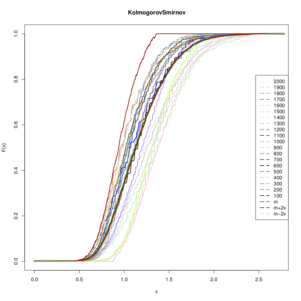
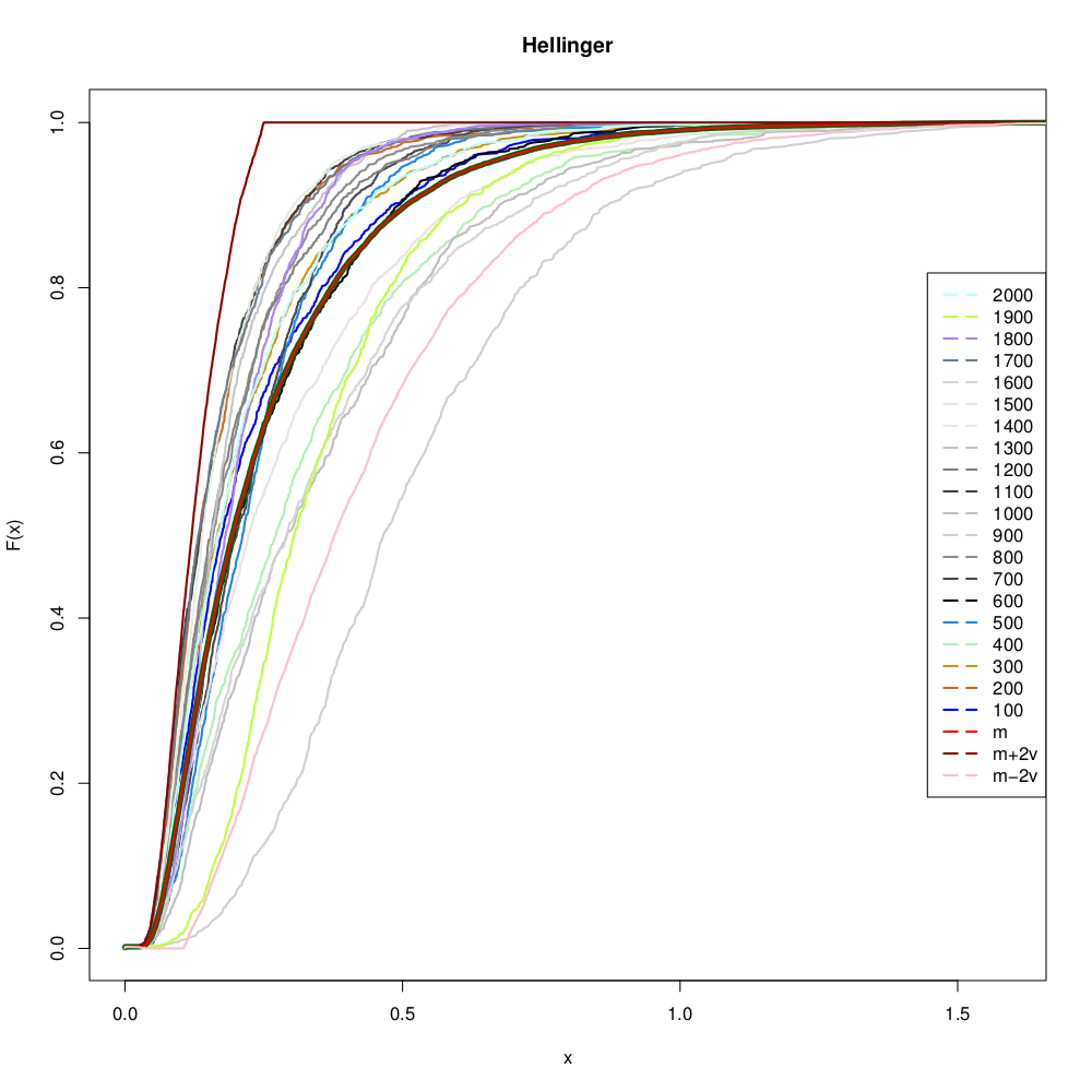
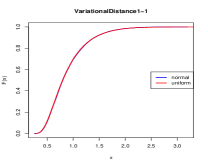
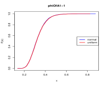
We present the results of the simulation of the Kolmogorov–Smirnov () and Hellinger (H) measures in Figure 1 and 2, respectively. For window sizes between 100 and 2000, at increments of 100, we generated 1000 intervals drawn from the same normal distribution . Then we computed the value of the measures to determine the CDF that supports the similarity assumption .
In Figure 1 and 2, for window sizes (dark blue) and (azure), both measures have CDFs that are similar. This is made possible because of .
Average . For each window size, we have a different CDF . We define the average of the distribution as,
| (39) |
Notice that is still a distribution and it could be considered as representative of the family of distributions (e.g., even though is not a valid distribution, is). In Figure 1, we draw the average in red. With our assumption about the nature of the distribution function, should tend to .
Variance . A natural definition of distribution variance is
| (40) |
In general, is not a distribution. Furthermore, the use of subtraction and power prevents the result from being a valid distribution, because the resulting can be negative for some . In Figure 1, we plot in dark-red, and in pink.
We assume that we have found a representative distribution when at least 19 of the 20 CDFs, 90% of them, are included in the intervals . This suggests that the CDF functions have a normal distribution . So, as gets larger, this should converge to our assumption . Recall that empirically, should be a smooth function that does not exhibit any anomaly accumulations or steps because of the merging of with different . Thus, we may consider to be the representative distribution function of the measure. 777Note that in practice, we could not find a CDF for the Bhattacharyya measure because we could not find a smooth CDF.
5.3 Input Distribution Independence
Let us consider the output of a CDF to be a stochastic variable and refer to as . Now, assume that is the inverse function of , properly defined for a finite number of samples . Then the event is identical to the event , which has the probability . This leads to for (see [Feller (1971)] Ch.1 Section 12). Thus, when we consider the input , we actually obtain a measure for which the distribution of the input should not affect the distribution of the measure, because is uniformly distributed independent of .
What we have found experimentally is that is independent of the distribution of the inputs and , as we show in Figure 3. Moreover, the distribution function can be used as a representative distribution.
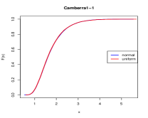
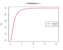


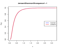
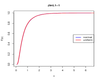
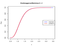
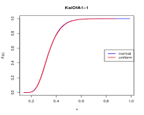
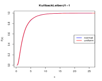
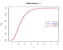
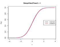
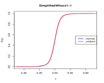
We repeat the simulation described in Section 5.2 for window sizes 100–2000, collecting 1000, 2000, 5000, and 10000 samples per window size, while using two different stochastic processes, a normal distribution () and a uniform distribution (). For each stochastic process, we obtain four representative distribution functions. We then compare the results in a table (by size and input distribution), and report the first tile only (1000 samples per window size) in Figure 3 due to space restrictions.
By applying the standard measures, the same measure described in this work, and by simple visual inspection, we can say that these new stochastic distance measures have a distribution that is independent of the window sizes and the distribution of the process we compare. This gives us compelling evidence that our measures, such as JS, have a measure distribution that need to be pre-computed by simulation and only once.
We use the larger set (with 10,000 samples) to determine different -values, and then determine the measure thresholds for each -value. For example, we determine the threshold value having a -value of 95% for each measure. In practice, this means that if we generate and from two intervals and , and apply the measure , then if that measure has a value that is larger than the threshold, we know that only 5% of intervals drawn from the same stochastic process will have the same or larger measure. However, we may still decide to reject the assumption that and are similar because the probability is too small.
In the following experiments, we use the simulation distributions to tabulate the -values and the significance for each measure.
5.3.1 Disagreement (with Multiple Measures)
A measure is designed to detect and to quantify the differences between inputs. Different measures are sensitive to different properties of the inputs, and therefore, they do not all perform alike.
We investigate and quantify how the aggregation of different measures can affect the sensitivity of a non-parametric measuring system. Consensus is a simple approach by which we can use different measures and make a decision only when a quorum of the measures agree. All the measures presented in this paper are designed to perform better at verifying that two distributions are statistically equivalent (the hypothesis is true); otherwise, there is no equivalence.
We quantify the detection power of different measures and determine the minimum quorum or rate for consensus (e.g., 10% disagreement means that only 1 measure in a set of 10 suggests that the two distributions are different, 90% agreement). In particular, we want to show that our extensions of measures, as proposed in Section 4.1, are a good contribution.
In the following section, we discuss the experimental setup and results (see Section 8).
This Section’s references are [D’Alberto and Dasdan (2009), Ali and Silvey (1966), Golub and Loan (1996), Lin (1991), Lee (1999), Wang et al. (1992), Jones and Furnas (1987), Shivakumar and García-Molina (1995), (41), Kullback and Leibler (1951), Jensen (1906), Shannon (1948), Kagan (1963), Vajda (1972), Hope (1968), Hahn (1912), Bhattacharyya (1943), Kailath (1967), Pinsker (1960), Chernoff (1952), Taneja and Kumar (2004), Kolmogorov (1933), Kendall (1991), Feller (1971), Kifer et al. (2004), Melucci (2007), Anderson (1962), Batchelor (1978), Wilson and Martinez (1997), Diday (1974), Wilson and Martinez (1997), Wilcoxon (1945), Mann and Whitney (1947), Harel (1993), Takács (1991), Feller (1948), Chakrabarti et al. (1998)].
6 Experimental Results
7 Multi-dimensional Experimental Results
In this section, we present the experimental results for multi-dimensional series. For clarity, the discussions in this section are further separated into the following topics: series generated from synthetic data (Section 7.1), series generated from classified data taken from UCI databases (Section 7.2), series generated from hardware counters for search engine properties (Section 7.3), and series generated from historical stock quotes (Section 7.4).
Note that for the first two data sets we have a full understanding of the series data. We use this knowledge for the validation of the methods and their discriminative capabilities. Specifically, we want to apply the methods to detect the differences between benign and malignant cancer. For the last two data sets, we are more interested in finding the similarity of series. Specifically, identifying similarity in the hardware counter data helps to group applications based upon run-time performance properties. For stock quotes, we show how the methods can be applied as scan statistics [Glaz et al. (2001)].
In the following, we describe the experimental set up for each method.
MST/Poset Method Set Up. The MST and poset-based methods compare the empirical CDFs using a quorum of the following ten measures: , , KS (Kolmogorov–Smirnov), KLJ (Kullback–Leiber–Jeffrey), JS (Jensen–Shannon), , H (Hellinger), (Cramér–von–Mises), E (Euclid), and C (Camberra). We set the ratio for rejection by the quorum to 20%, meaning that at least two measures must reject the equality hypothesis for the quorum to reject the hypothesis (see Section 3.5 or [D’Alberto and Dasdan (2009)]).
Compression Method Set Up. We create a -value range by bootstrapping using 100 runs. The training set and bootstrapping process are described in Section 3.2.1. Bootstrapping is performed for every series that we present.
Martingale Method Set Up. We set the following parameters: , , and for the Martingale method. Recall that is the maximum value of the Martingale value before a change is declared, is the confidence margin used in rejecting the equality hypothesis even though the hypothesis could be true (in this case, a maximum of 5% error is tolerated), and is the maximum increase of the Martingale value in a single step. In practice, , , and are tunable parameters in conjunction with the size of the reference interval .
Kernel Method Set Up. Having decided upon the Gaussian kernel, we need to determine the value of the variance parameter . The value of this parameter is estimated from the data of all the series. As for other methods, the significance -value of 5% is used.
7.1 Synthetic Variation
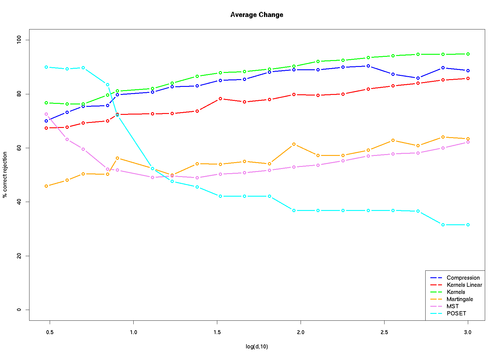
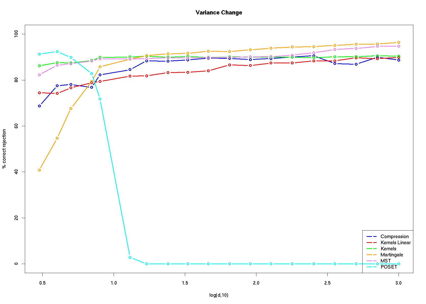
We created three tests, similar to the experiments conducted by other researchers. The tests are a change in average only, a change in variance only, and a change in distribution from normal to uniform. We took a series and divided it into 21 intervals, each consisting of samples points. We chose to use 250 sample points per interval to keep the tests compatible with experiments presented in the previous work. The first two intervals are drawn from the same stochastic process, which has the normal distribution . These two intervals can be used to bootstrap the compression method or to tune the Martingale method. Nonetheless, it is a pre-requisite that all methods recognize these two intervals as equivalent.
We constructed the series such that we increased the average, the variance, or the distribution mix as the series progressed. We also investigated the relationship between the dimensionality and the sensitivity of the method to identify the variation as early as possible. That is, for each method we measured the average shortest time or the least number of data points necessary to identify the artificial change.
For each series, the first interval is the reference interval , and does not move; while the moving interval slides through the series. For all methods, except the Martingale method, the moving interval shifts by a full interval window size. The Martingale method scans the series one point at a time.
The summary results displayed in Figure 4 were generated in the following manner. For each method and each of the three types of series change, we ran 100 simulations. Two such results are presented in Figure 5 and Figure 6. We recorded the earliest time stamp when a method first identified a variation and rejects the similarity hypothesis. More detail will be provided in the following sections.
The rejection rate is computed as the ratio of the earliest time to the overall length of the series. We define the ratio as:
where is the number of samples in an interval, =; recall that the first two intervals are drawn from the same distribution and thus we must remove points from the overall series.
Figure 4 presents the effect on the average early rejection rate as the dimensionality of the series increases (on a logarithmic scale).
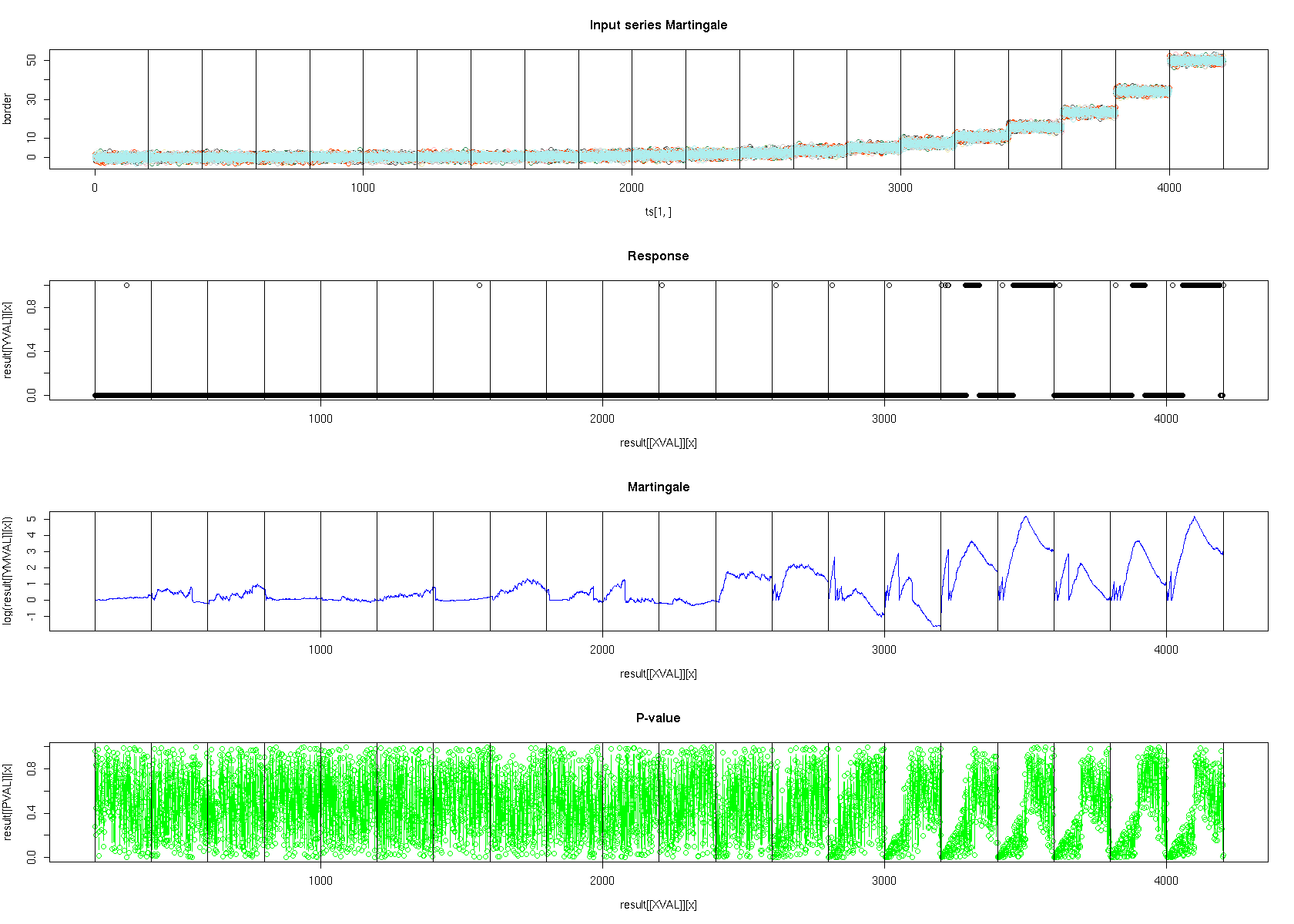
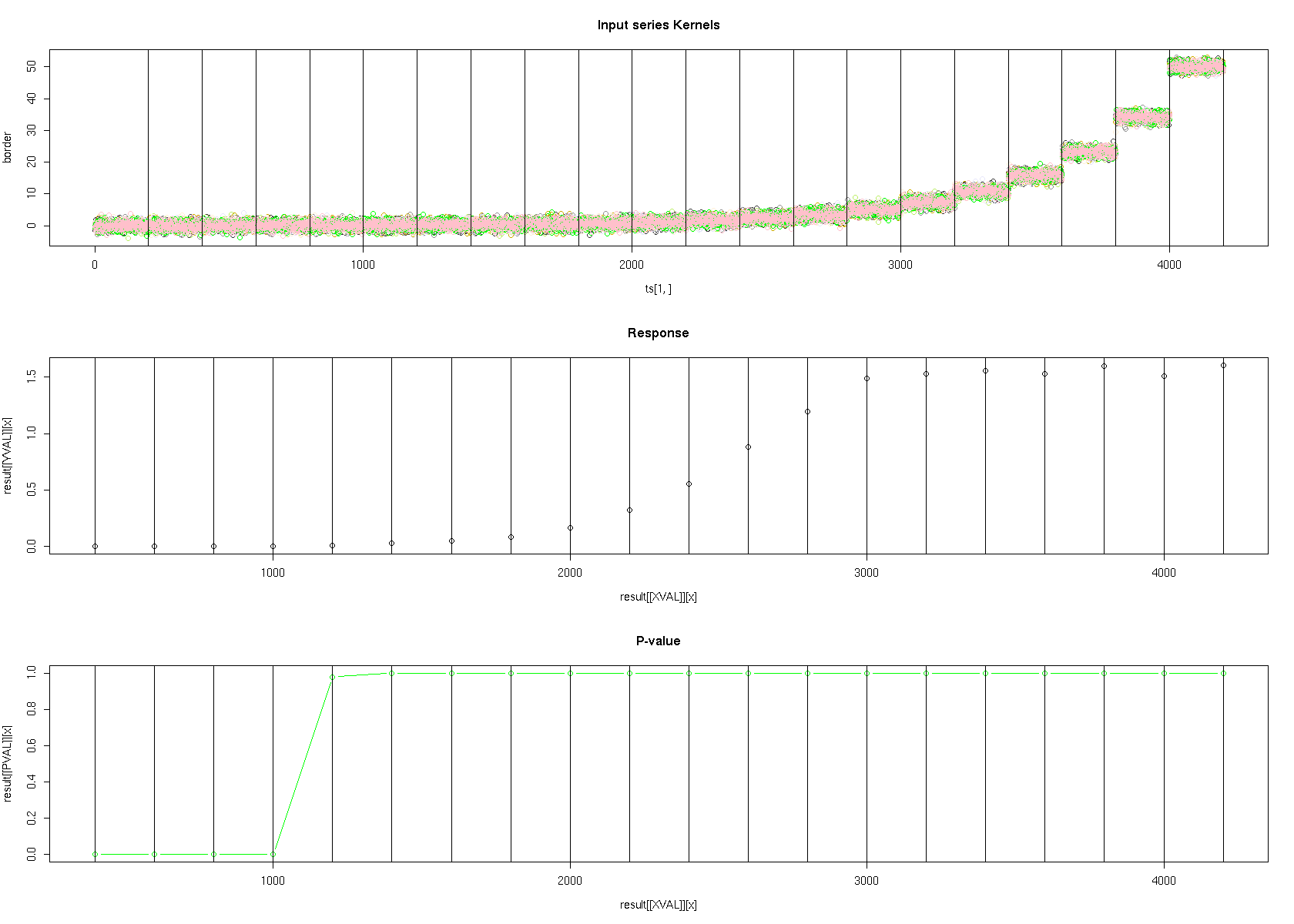
7.1.1 Results for Changes in Average
In Figure 5, we show an example of a series and an excerpt of the responses generated by the Martingale method. The Martingale method response is composed of the following four series from the top to the bottom: The first series is the input; the second is the response, which indicates a difference when the value is 1, otherwise 0; the third is the Martingale value; finally, the fourth series is the -value from the transducer, which is the estimated probability distribution.
We also show an excerpt from the Kernel method, similarly displaying the input, the Kernel value, and the -value. A -value larger than indicates a change with 5% confidence.
As mentioned above, we created 21 intervals from a normal distribution with average values logarithmically spaced over the range of 0.05 to 50. Clearly, the earlier a method discovers a change in the average, the more discriminating the method is. The overall performance is shown in Figure 4. The details are discussed further in the summary section.
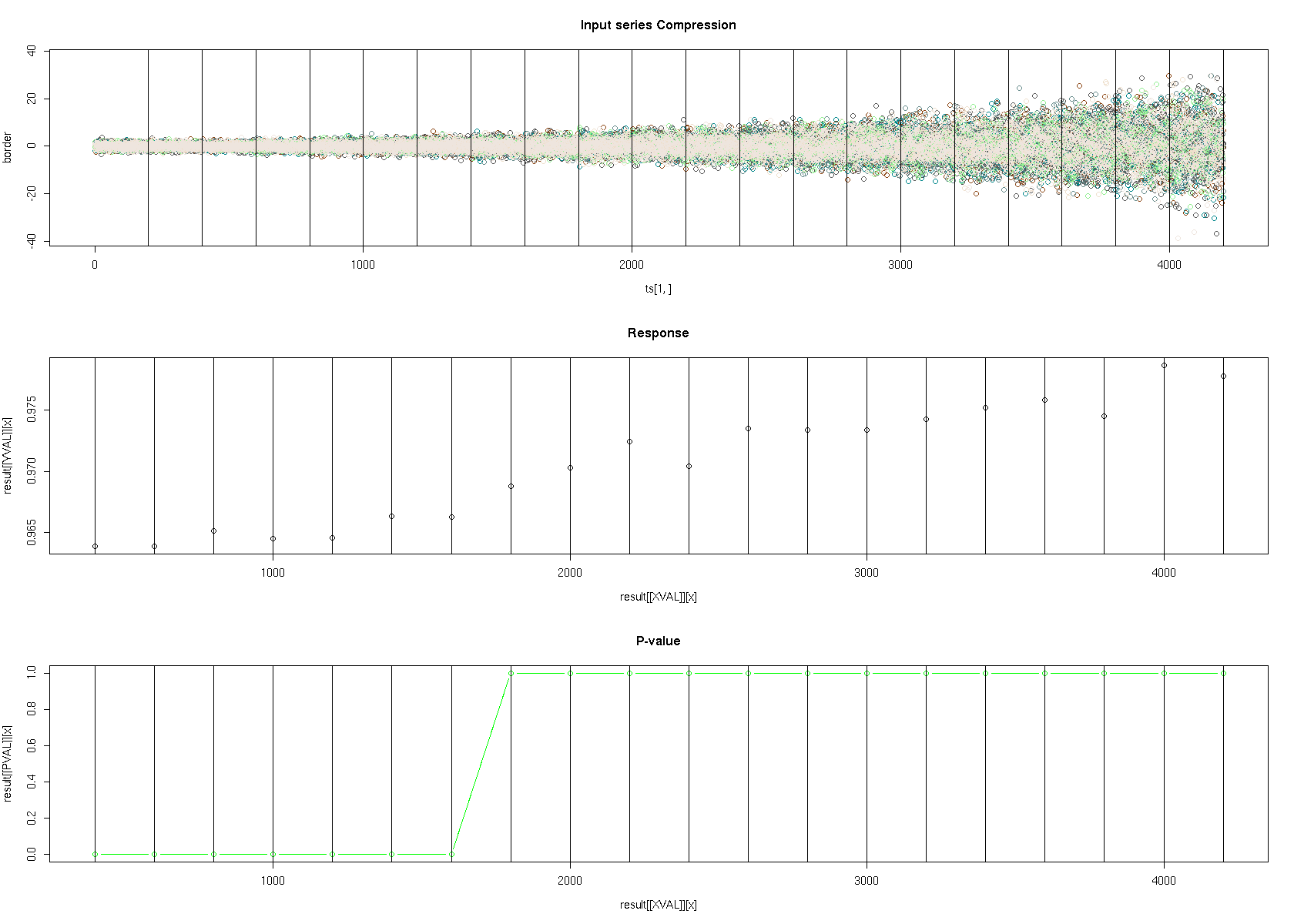
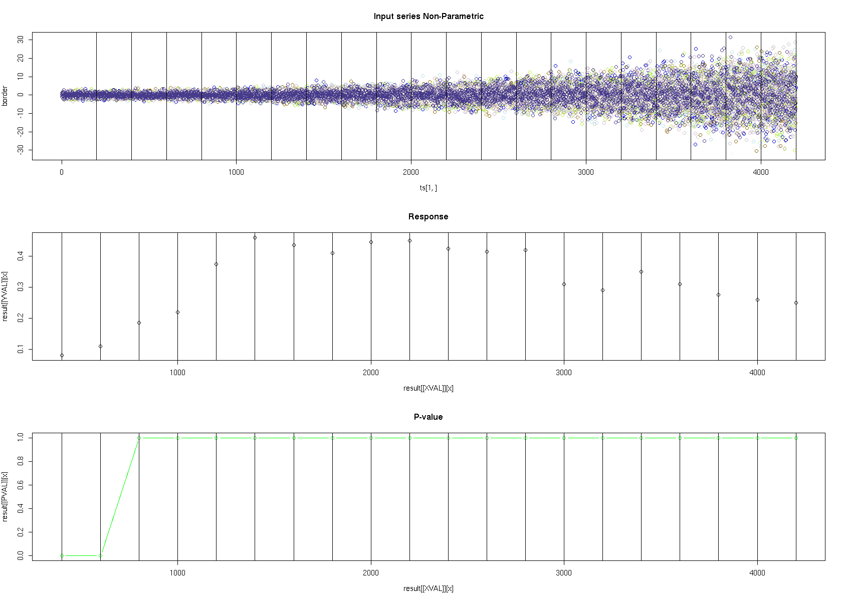
7.1.2 Results for Changes in Variance
In Figure 6, we show an example of a series and an excerpt of the responses generated by the Compression method. The Compression method response is composed of the following series: the input, the NCD value, and the -value as computed during bootstrapping with 100 samples. We also show an excerpt from the MST method, displaying the input, the minimum distance across 10 built-in tests, and the 20%-quorum based -value, generated from the -values of the quorum measures.
Similarly as in the previous tests, we created 21 intervals from a normal distribution with a null average and variance values logarithmically spaced over the range of to 10. Clearly, the earlier a method discovers a change in the variance, the more discriminating the method is. The overall performance is shown in Figure 4. The details are discussed further in the summary section.
7.1.3 Results for Changes in Distribution
This is the last of the tests on the synthetically generated data sets. The purpose is to quantify the ability of each method to identify when the distribution changes (average and variance do not change significantly). We start with an interval generated by a normal process with distribution . With successive intervals we mix points generated from the uniform distribution , in such a proportion that all the points in last interval are generated by the uniform distribution.
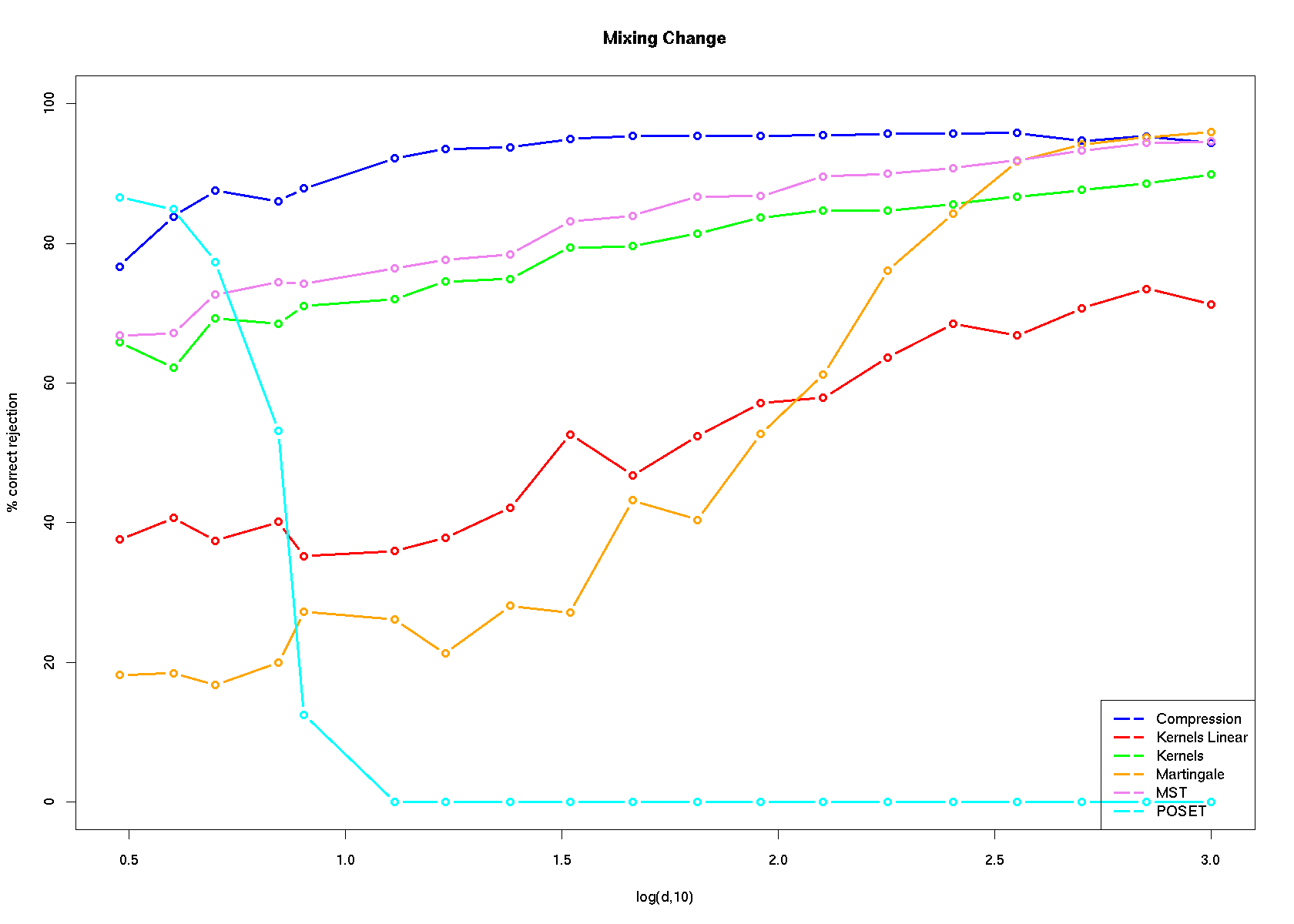
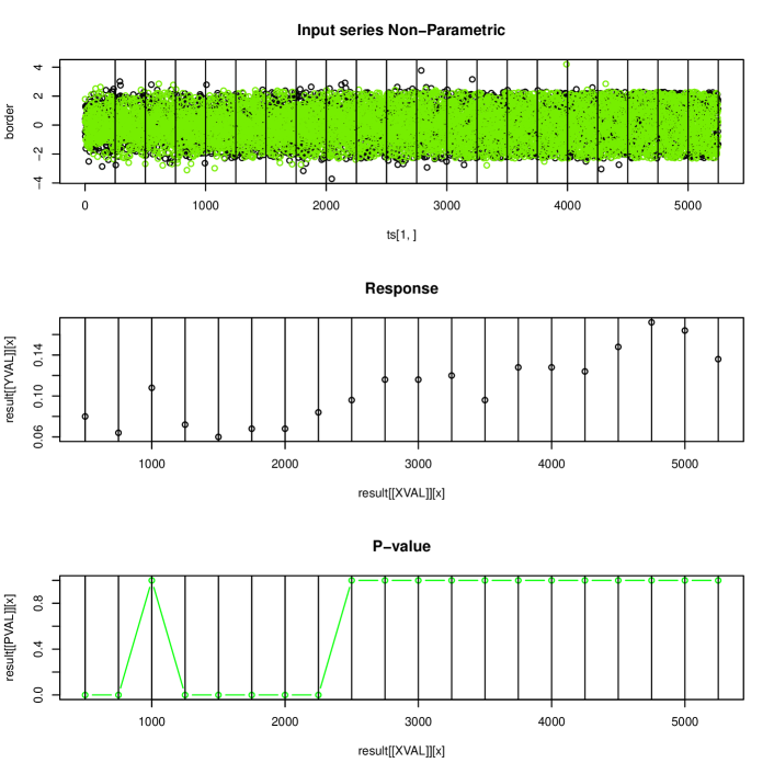
As per the above tests, the first two intervals are drawn from the same process. We gradually decrease the number of points from the normal distribution by a factor of 1/20, while increasing the points from the uniform distribution by the same factor. This results in a gradual transition from a normal distribution to a uniform distribution. We repeated this process 100 times. Then we increased the number of dimensions of the series so to test the effects of dimensionality. In Figure 7, we show the average early detection of distribution change for all methods (above), and an example of the responses of the poset method on a two dimensional data set (below). The response consists of the input, the minimum distance across 10 built-in tests, and the 20%-quorum based -value, generated from the -values of the quorum measures.
7.1.4 Summary of Synthetic Data Results
Here, we present our conclusions from the average, variance, and distribution tests described previously.
-
•
The methods exhibit different sensitivity to changes in average and variance; they tend to be more sensitive to changes in variance.
-
•
Although the poset method has the best discriminative power for few dimensions, it does not scale well. When a series has more than 10 dimensions, the method is not able to detect any changes in variance or distribution. The reason for this can be understood if one considers a selection of points in ; the probability of finding them in any particular order is very small. In practice, the partition of the topological ordering is composed of a few sets (3–5), too few to draw any conclusions.
-
•
The MST method is not very consistent. Although it performs poorly for detecting changes in average, it is the second most powerful method for detecting changes in variance or distribution. As the dimensions increase, the performance of the MST method improves. Because the MST method is based on the relative distance between points, the information gained from the distance between points increases with more dimensions.
-
•
The Kernel method performs consistently well and outperforms other methods for detecting change in the average.
-
•
The Martingale method works best for changes in the variance, but not so well for changes in the average. Notice that the moving window is relatively small and the transducer output, the -value, has relatively short changes. Consequently, the Martingale value cannot reach large values, there is minimal skew in the -value distribution, and the change is difficult to detect. However, for the variance test, the -value tends to be small because the new point is often out of the range of the moving interval (in this scenario the Martingale increases fast and the -value has a skewed distribution).
-
•
The Compression method works well because bootstrapping is done before every run. The bootstrapping tunes the method to the properties of a particular series.
-
•
For the distribution test, the linear Kernel method performs poorly. The Martingale method performs poorly on small and medium dimensions because the -value of the transducer does not change enough to prevent the Martingale value from being reset to 1 (this is a problem with our implementation more than a failing of the method). However, the Martingale method does work well on large dimensions. The full Kernel method generally works well. The best method for the early detection of change is the Compression method. The poset for very small dimensions, and the MST methods for all dimensions are the best non-parametric methods. This comes as no surprise, as these methods are designed to capture changes in distribution.
Sample Size and Dimensionality.
Rejection ratio median for series in , based on 100 runs, with change in average and an increasing number of points in each interval Method N=250 N=500 N=750 Compression 0.77 0.83 0.84 Kernels 0.81 0.85 0.87 Kernels Lin. 0.73 0.729 0.75 Martingale 0.50 0.66 0.73 POSET 0.66 0.76 0.79 MST 0.49 0.49 0.49 MST (variance) 0.89 0.90 0.89
In the previous tests, we fixed the length of the interval and change the dimensions. The length of the interval is the same used in previous work. In this section, we present an introductory study about the relation between the interval length and the number of dimensions of each point in the interval, see Table 7.1.4.
As we expected, increasing the number of points means there is more information about the process being measured, which results in the methods being more discriminative. The exception to this rule is the MST method, as explained in Section 3.4.2. Although the poset and MST methods share the same statistical tests, they order data differently. In the case of the MST method, having more points does not change the inherent structure of the MST, and therefore does not impact its discriminative ability.


Sensitivity: Early Rejection Versus Total Number of Rejections.
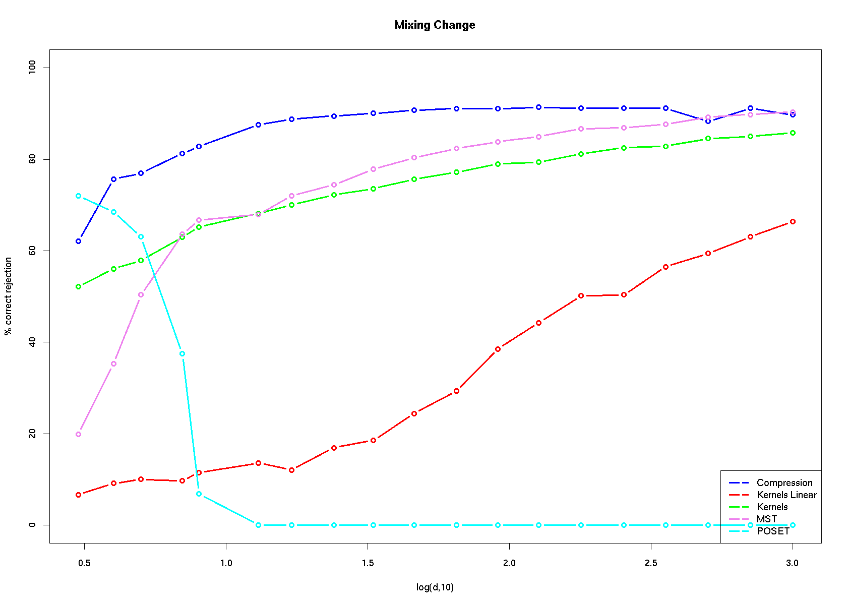
Excluding the Martingale method, we can compute a sensitivity measure for each method by counting the number of times a method identifies a change (instead of how early a method detects a change). Recall that 21 intervals were constructed where the first two intervals are intentionally similar (to the reference window) for the purpose of tuning the method. As the moving window covers a single interval, we expect each method to identify 20 changes.
Figures 8 and 9 present the sensitivity measure. As before, the methods tend to become more sensitive as the number of dimensions increases, excepting the poset method for reasons mentioned previously. Again, the poset method is the most sensitive for series with fewer than 10 dimensions.
As expected, the methods are consistent in the sense that an early discrimination translates into a better overall discrimination.
7.2 Pre-Classified Data
In the previous section, we explained how we created synthetic data sets with known properties, such that we could control the introduction of differences caused by changes in average, variance, and distribution. In this section, we present a method for creating data sets with well known properties based upon pre-classified data. We use four freely available data sets from the UCI machine learning repository [Frank and Asuncion (2010)]. We used the following data sets: yeasts with nine dimensions (also referred to as attributes in [Horton and Nakai (1996)]), abalone with eight dimensions [Nash et al. (1994)], Parkinson’s disease with 26 dimensions [Tsanas et al. (2010)], and breast cancer with 30 dimensions [Street et al. (1993)].
We selected these data sets for several reasons, including the fact that they have a managable number of dimensions, literal dimensions can be easily translated into numerical values without any loss of information, and we can safely assume that the attributes come from a continuous distribution.
From Data Set to Series. For each data set, we grouped the data into intervals by using the class identifier as the partitioning key; for the Parkinson’s disease data set we include the person identifier in the partitioning key. We concatenate these intervals in decreasing length order. In practice, the first interval will contain the largest number of points, while the last interval will contain the fewest. For each interval we perform a random permutation of the points, which helps to break down any previous bias within the interval. In the experiments we use a moving window with a size that is often smaller than the intervals.
We tested our six methods using four different moving window sizes. For the breast cancer data set we used window sizes of 50, 100, 200, and 300; and for the other data sets we used window sizes of 100, 200, 300, and 400. The results are presented in Figure 11, 12, 13, and 14.
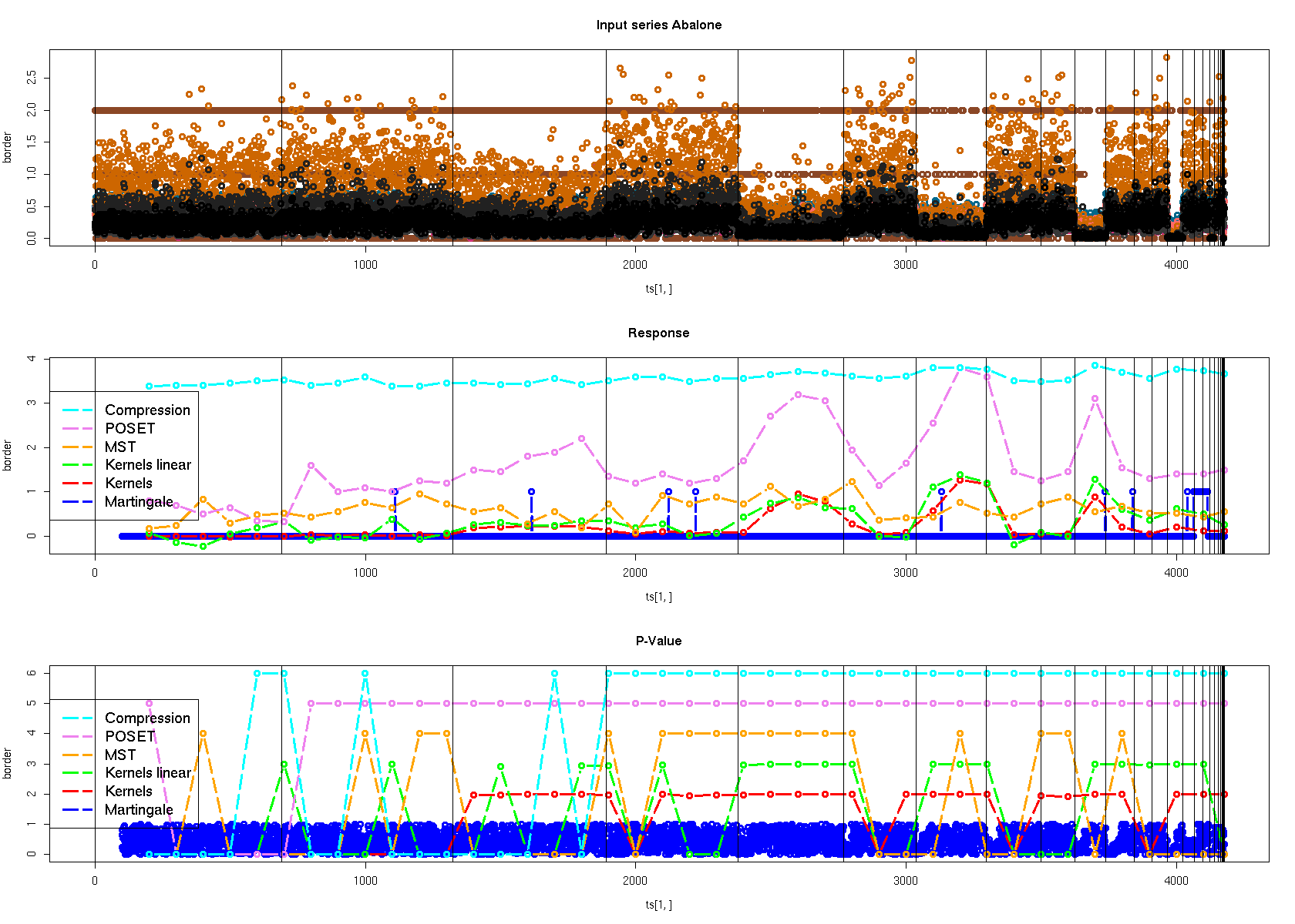
To ease the introduction of the data sets and the application of the methods, we turn our attention to the abalone data with window size 100, see Figure 10. We shall take the same steps for the other classified data set.
First, we start describing how we represent the input series, which is always the first scattered plot in each figure. We use colors to plot the different dimensions of the series in order to capture more facets of the data. We mark the borders between intervals by using a vertical line, making it easy to distinguish the known classifications. For example, for the abalone data, we have 21 different intervals with different lengths.
Second, we shall show the response of every method. The response from the Martingale method is encoded in the response row, where a value of 1 indicates a difference and 0 indicates no difference. For the other methods, we plot a normalized distance measure as we shall explain shortly for the -values. For example in Figure 10, the Martingale method flags a difference at: 1100, 1600, 2100, 2200 and after 4100. Notice that the first four differences are false differences because the moving window is entirely contained into a classified interval. The last differences are actually correct. In the following, we shall present performance with a window size of 400 points: with a larger window we shall capture better the variations of larger classified intervals but not for smaller ones having the opposite situation that the one presented here.
Third, we report the -value. A -value larger than 0.95 indicates a significant change. To encapsulate all of the change responses for the methods in a single figure, we draw -value on a single plot, where is an integer in and is uniquely associated with a method (the response is computed similarly) and color coded for easy consultation. A rejection is represented by a rise of the -value line to .
Therefore, if all the methods reject all the intervals, then the resulting plot will show six parallel lines on the interval 1–6. Recall that the only exception is the Martingale method, for which we use the -value of the transducer in conjunction with the response.
For example in Figure 10, The first interval of 100 points is taken as reference, then we let the moving window scan the series with interval of length 100 points. The poset method (pink line) detects a difference within the first interval, which is false; however, the poset method detects correctly all other interval as different. The compression method detects two false differences, but overall it is capable to find always a small window in each classified interval that is different from the reference. Notice that every method detect a difference when the moving window is scanning the interval 2400–2800: we can see five parallel lines.
Obviously, our goal is to show that we can distinguish between different classified intervals. However, the differences in the interval lengths cause problems to the scanning methodology, as the moving window may be too large that it spans multiple intervals or may be too small to completely cover other intervals. In this case, we show that the reference window is from a single interval and is different from a combination of intervals. Recall that the reference window and the moving window are of the same size and we shall present results for different sizes.
Note this section is meant to provide a qualitative presentation of the discriminative powers of the methods.
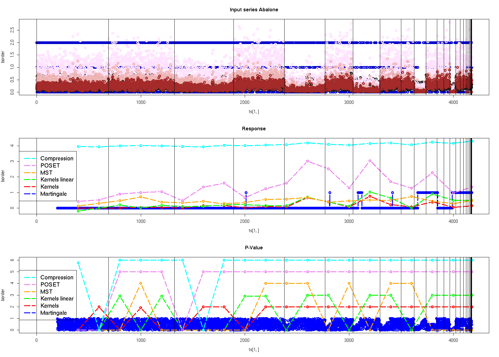
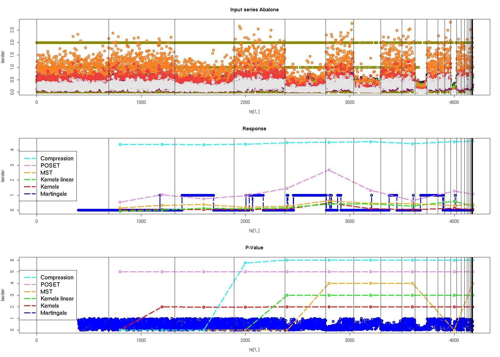
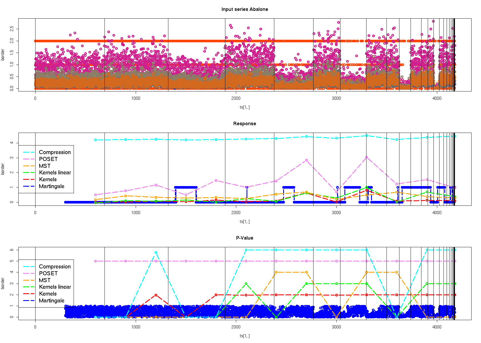
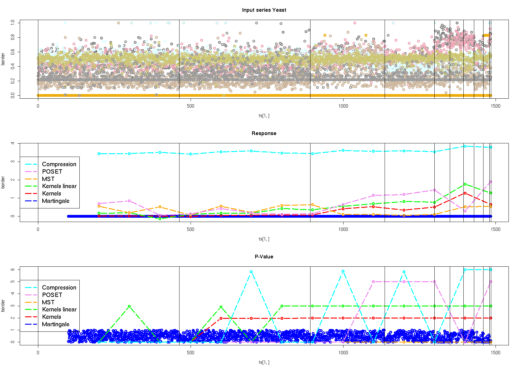
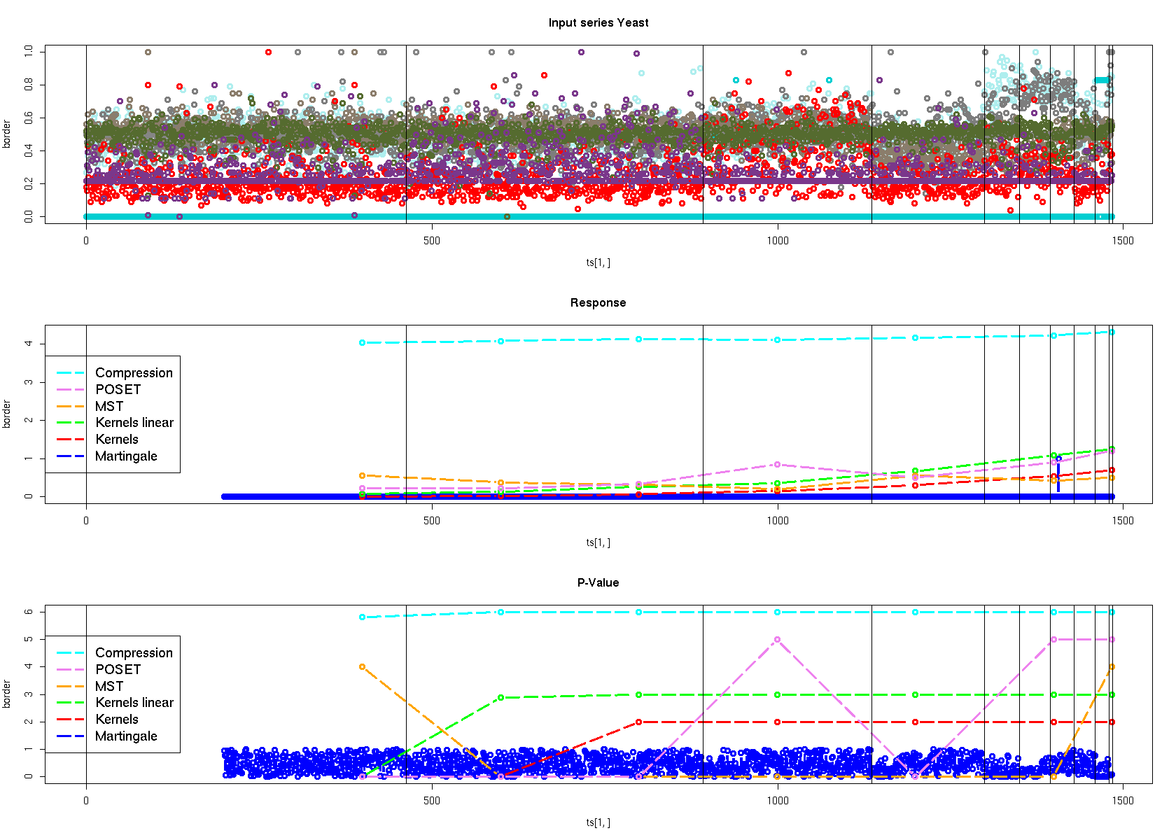
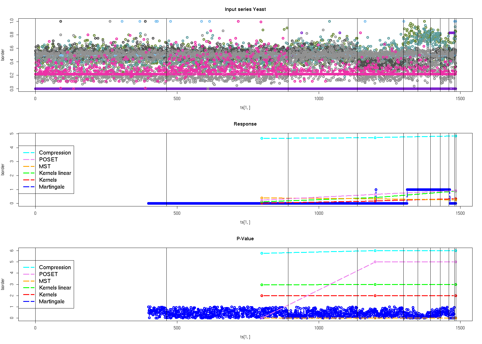
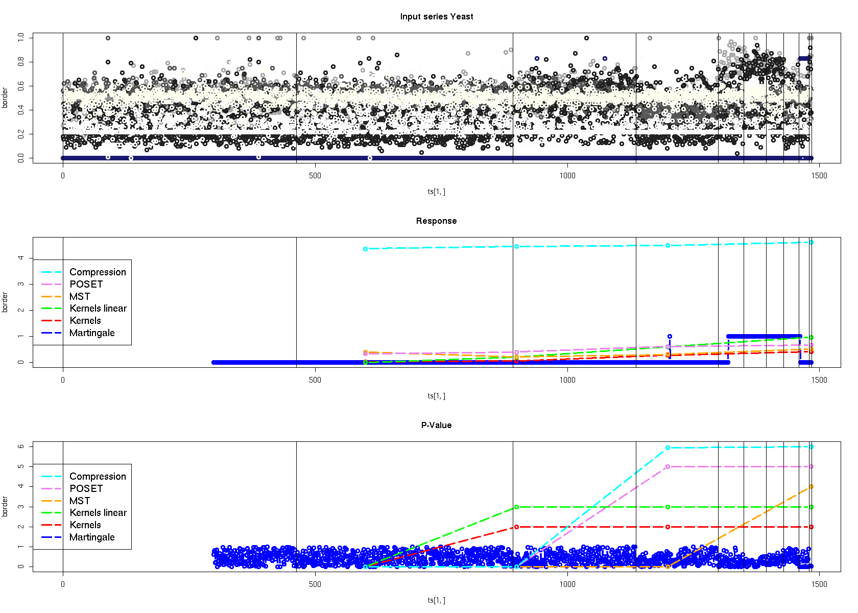
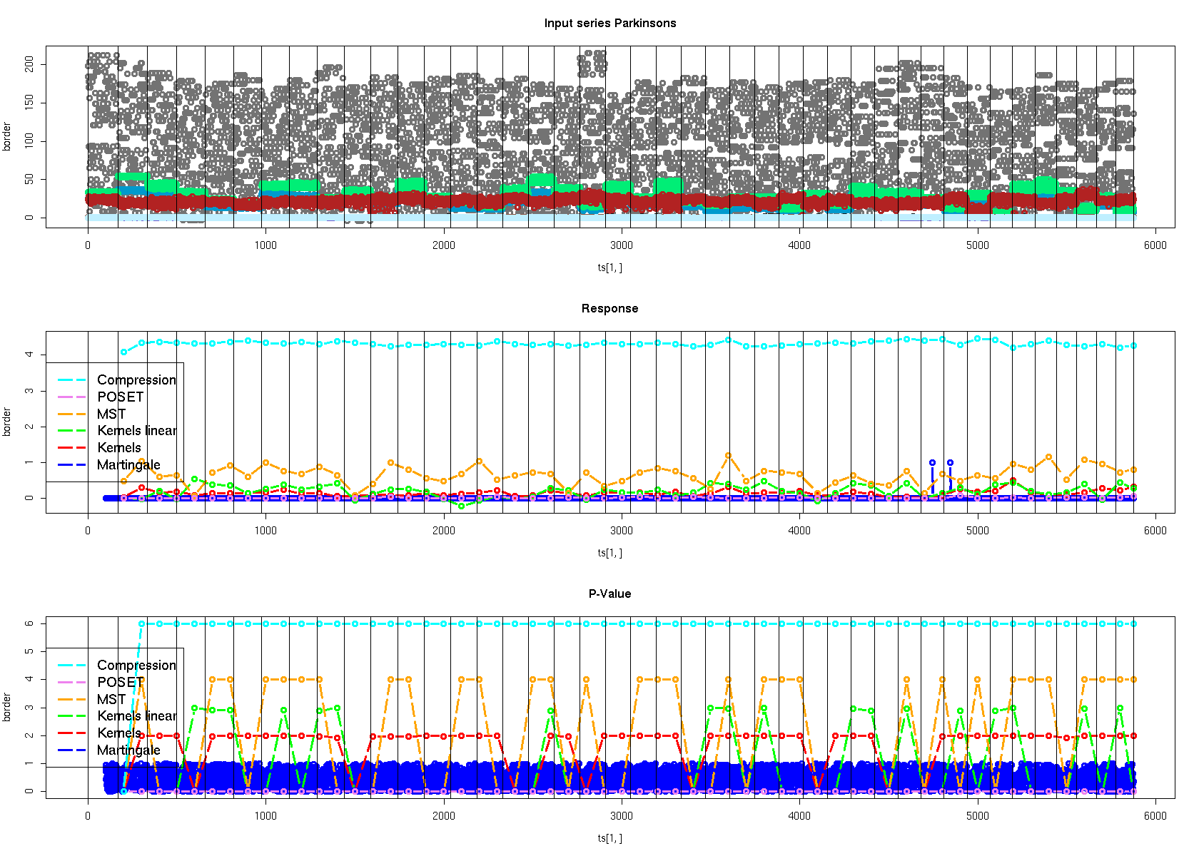
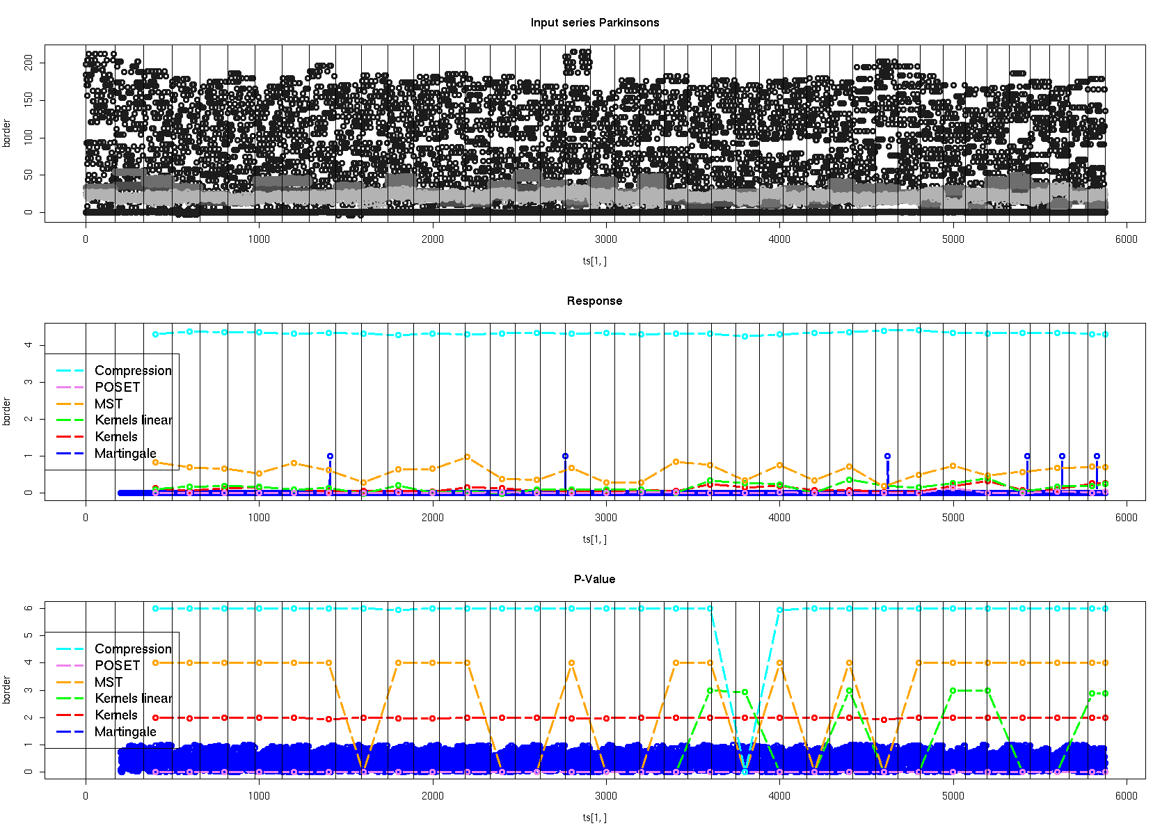
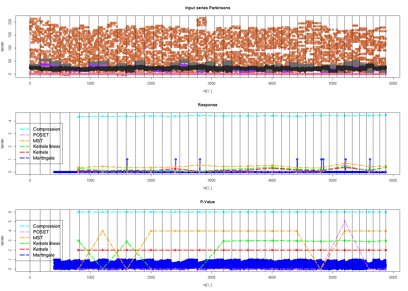
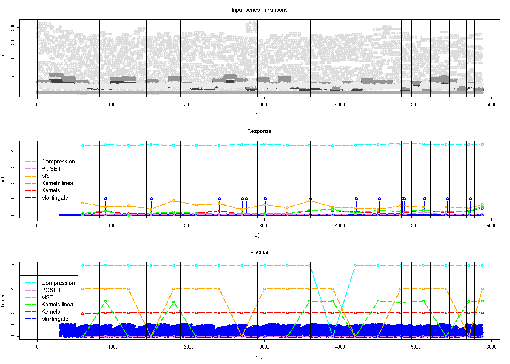
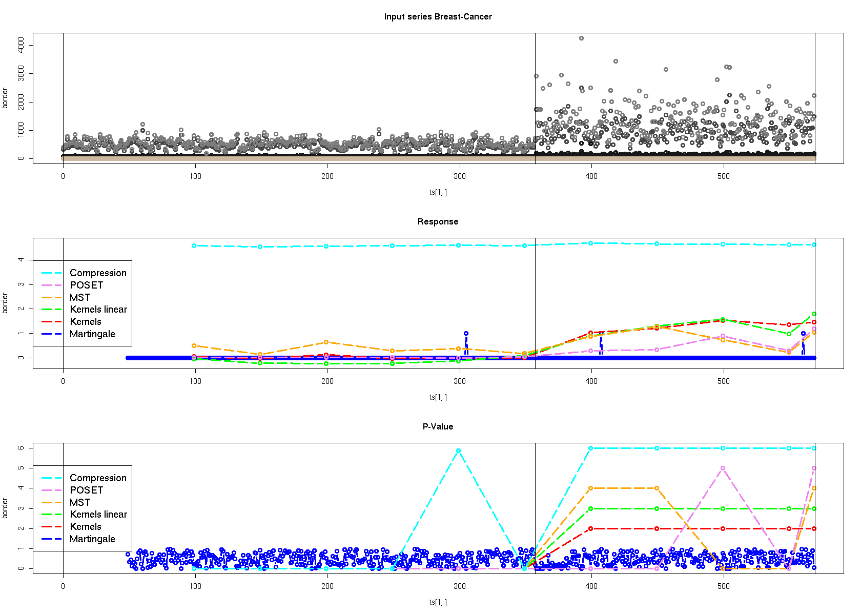
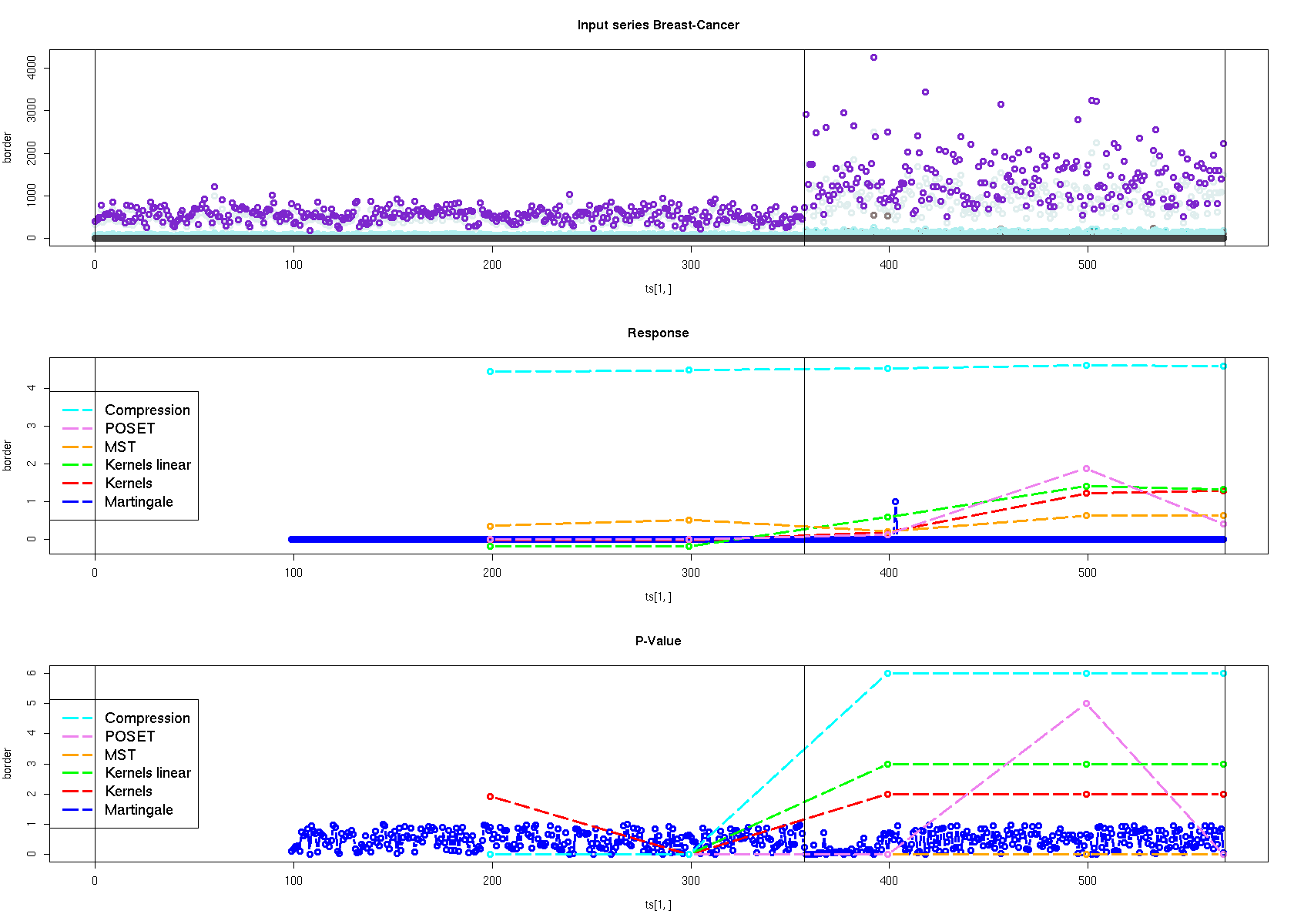
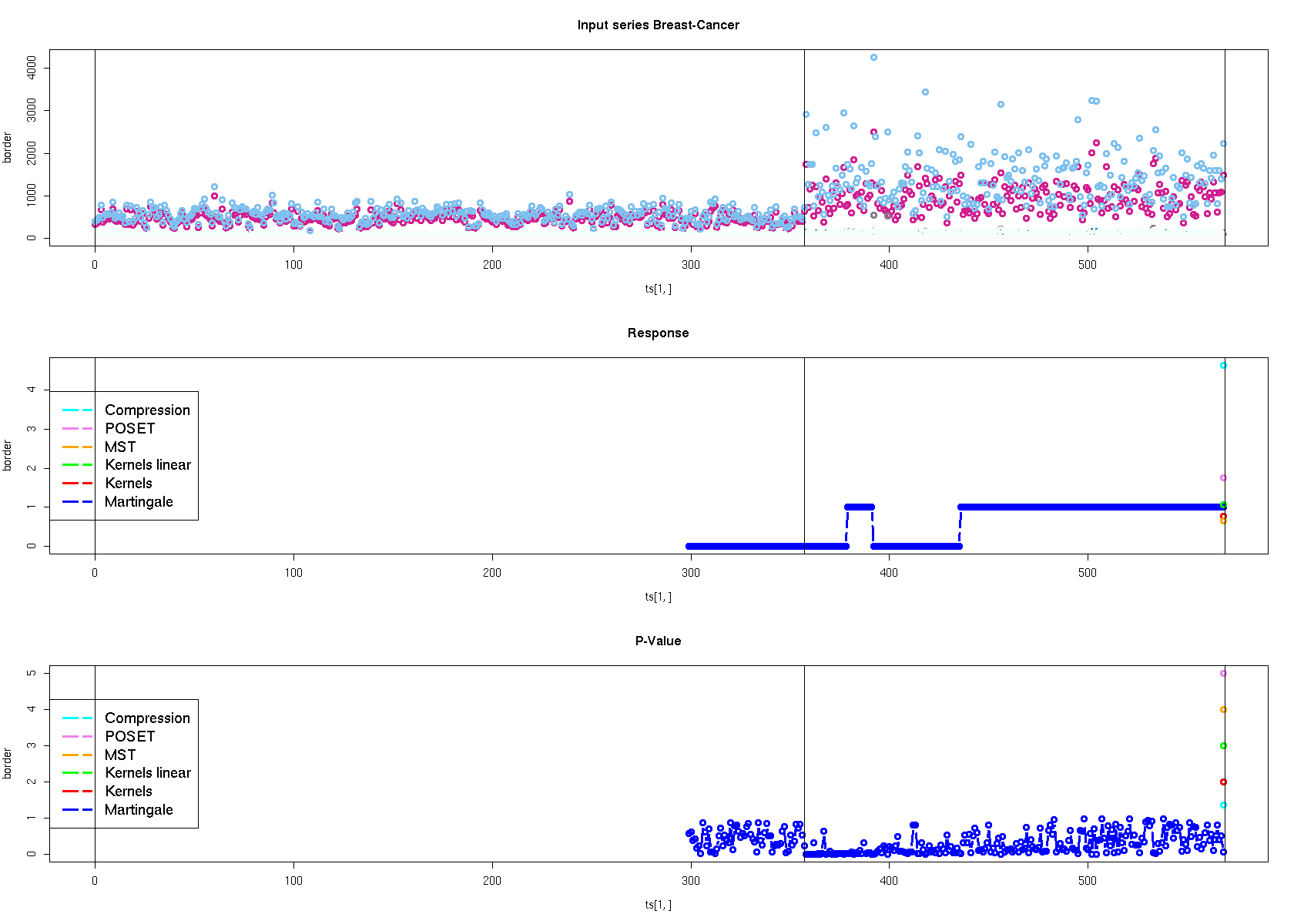
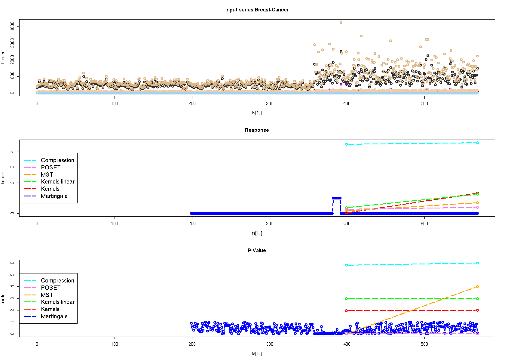
Abalone Data Set, 8 Dimensions. In Figure 11, we identify an interval based on the age of the abalone. The series is generated by concatenating the intervals in decreasing order of the number of points. The sex attribute is transformed into an integer value of 0, 1, or 2, where the mapping is arbitrary but fixed across the tests. The first interval contains enough points to perform bootstrapping for the Compression method. We present the responses for different window lengths of : 100, 200, 300 and 400. When , the moving window is able to cover almost every interval. We notice that, aside from a single false negative, the poset method always successfully detects the changes. The Martingale method performs well on the larger intervals, for which the moving window covers the interval, because it is able to capture the -value distribution change. The Kernel method performs well and the Compression method is consistent as well. As the and increase to 400 points, the discriminative powers of the methods also increase, particularly the Kernel method.
We discuss further the results we observed by putting them in the context of the properties of the methods that we presented in previous sections: this series presents a change of variance.
Yeast Data Set, 9 Dimensions. We created the intervals in the same manner as described previously; however, we excluded the database identification number and used the yeast type as the partitioning key. Notice that, for any moving window size, the linear kernel method is the fastest at identifying changes, even faster than the regular kernel method. The Compression method does well, while the MST method did not perform well, and the poset method required a window size of at least 300 to be able to consistently identify changes.
This series presents an average change.
Parkinson’s Disease Data Set, 26 Dimensions. We kept only the telemetry and motor-skill data, and excluded the age and sex attributes when using this data set. Each patient has 200 data points, see Figure 13. Note: A hierarchical classification of the patients into classes of the disease stage would provide a better/more-appropriate test.
Due to the number of dimensions, the poset method did not work and it does not find any distinction; however, the Compression, MST and Kernel methods worked well. Notice that the Compression response should be taken literally only for the interval which contains 100 points (the top left figure), because the bootstrap is built within a single class. For larger window sizes we considered a reference window of at most two patients. The Kernel method and the Compression method are the most consistent measures. The MST method’s rejection rate increases as the number of points in each interval increases. The Martingale method does not work well on this data for two reasons; the series is built on intervals that are relatively short, and the Martingale moving window will encounter -value changes often enough that it will become a normal behavior. In other words, we found that the -value distribution was indistinguishable from the stochastic measure on the -value, resulting in the Martingale value being reset to 1 at regular intervals. In this case, a more time sensitive approach should be deployed for the -value change to let the Martingale value fluctuate naturally.
One final note about the Parkinson’s disease data set. If we were interested in finding similarity among patients, such as identifying progression groups for the disease, such as early, advanced, and final, we would not use a method that always finds differences between the intervals above —i.e., because each interval represent a patient.
Breast Cancer Data Set, 30 Dimensions. We consider two types of breast cancer, benign and malignant, and sort the data by the number of cases in each class. Visual inspection of the data in Figure 14 shows that the series contains changes in both the average and variance. We should expect all methods to catch one type of change or the other. Despite the number of dimensions, the poset method was able to identify the two classes with as few points as 50. Notice that the Compression method has a single false negative for the smallest window (of 50 points), because there was not enough data for bootstrapping to allow the method to identify a difference in the largest window.
Summary. For series built from pre-classified data, we showed that our methods provide a set of powerful tools. The changes in the series are captured by the methods in a consistent manner for a different number of window sizes and a different number of dimensions. Furthermore, we can classify the changes of the series by noticing which methods find the changes.
7.3 Application to Hardware/Software Performance.
In this and the following section, we present examples of series for which we want to find similarities, when there is neither a priori classification nor known properties for the data.
Let us consider an application and an architecture . Assuming that we are interested in collecting a set of measures, such as processor stalls due to cache misses or cycles per instruction, that are aimed at measuring the execution times of . If we sample these measures during the execution of on , then we are generating a multi-dimensional time series. In this paper, we consider the six measures described in [Cammarota et al. (2011)], and generate 6-dimensional series. These measures account for the cycles spent waiting for resources, and directly account for performance losses.
Consider an application which is a property of Yahoo! We would like to find another application, which exhibits similar performance characteristics on the hardware architecture . In this experiment we used SPEC INT 2006, SPECINT, which is part of a larger application set [Henning (2006)]. We generate multiple series by concatenating the series generated by each application onto . We reduce the problem to one of verifying that a change exists in the series.
Designing a Series. The set of applications that we run consist of the Yahoo! application and the set of SPECINT applications . We run each application on the architecture with a representative set of inputs, and collect performance statistics by sampling the hardware counters. This process generates a series where each point is an average result in an interval that is close to the sample point. The series is the result of a deterministic, albeit complex, process. The fact that there is a random component to the series means that, although two series should be similar, it is extremely unlikely that two series will be the same.
A search property and a comparison with SPECINT: h264ref and perlbench are always different. Method/App astar bzip2 gcc gobmk hmmer libquantum mcf omnetpp sjeng xalancbmk Compression diff diff diff diff diff diff diff diff diff diff MST diff equiv equiv equiv equiv diff equiv diff equiv diff POSET equiv diff equiv equiv equiv diff diff equiv diff equiv Martingale diff diff equiv equiv diff equiv equiv diff equiv equiv Kernel Lin. diff diff diff diff diff diff diff diff diff diff Kernel diff diff diff diff diff diff diff diff diff diff
Value of Identifying Similar Series. If we can find an application that is similar to the application for the architecture , we may consider as being representative of in general. When another architecture is introduced that improves the performance of , we may conjecture that will also improve , and vice versa. Notice that it is not necessary to run either or on a prospective new architecture, because manufacturers will provide results for SPECINT.
As a pruning device, if does not improve , then will not improve either —i.e., very likely will not improve either.
Constructing the Series. To facilitate the tuning of the tools, we followed the same process described in Section 7.1. That is, and produce two series and , we create a new series (or in case has fewer points than ), where signifies concatenation.
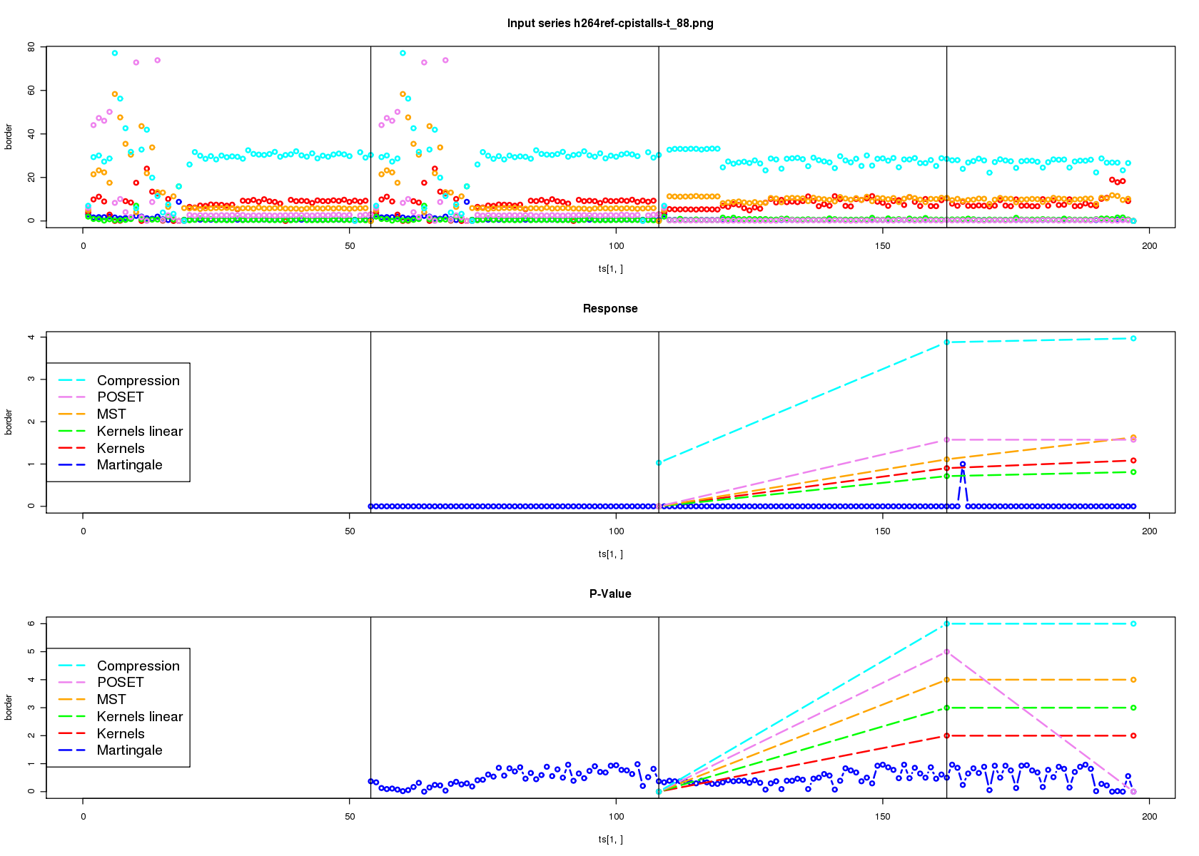
In Figure 15, we present an analysis using our methods where we compare our application (the tail of the series) with the applications (the head of the series), identified in the literature as h264ref. All the methods identified the two series as different.
In Table 7.3, we present the final comparison results for all the benchmarks. For this paper, we attach no specific importance to the application , as long as it is not from . In principle, we know that a discriminative method would differentiate from any application in SPECINT. In fact, the Kernel method and the Compression method, which take into account the evolution of the series over time, find no similarity (see Section 3.3.2 for a reminder of the linear Kernel method).
For the Martingale, MST, and poset methods, the evolution of the series over time is relative; and by contrast these methods are more sensitive to the frequency of the events. As a result, these methods find similarities that may not be apparent in the series. From our observations, we find that our application is similar to gcc, gobmk, and less similar to mcf, sjeng, and xalancbmk, because at least two different methods suggests a close similarity.
Summary. In this section, we introduced series that represent the performance of software applications and the interaction with the hardware that runs them. If we are interested in identifying the evolution of the series over time, then we should consider the Kernel method or the Compression method as candidates. If we are interested in identifying the similarity of distributions, then we should consider the MST or poset method. If we are interested in interchangeability, then the Martingale method is more appropriate. Here we used all the methods and a quorum to infer similarity among series.
7.4 Stock Market Quotes
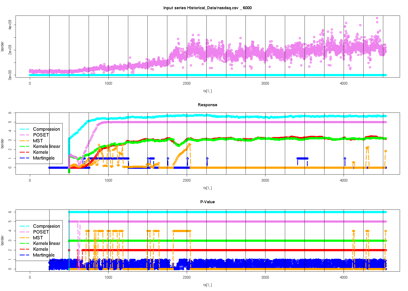
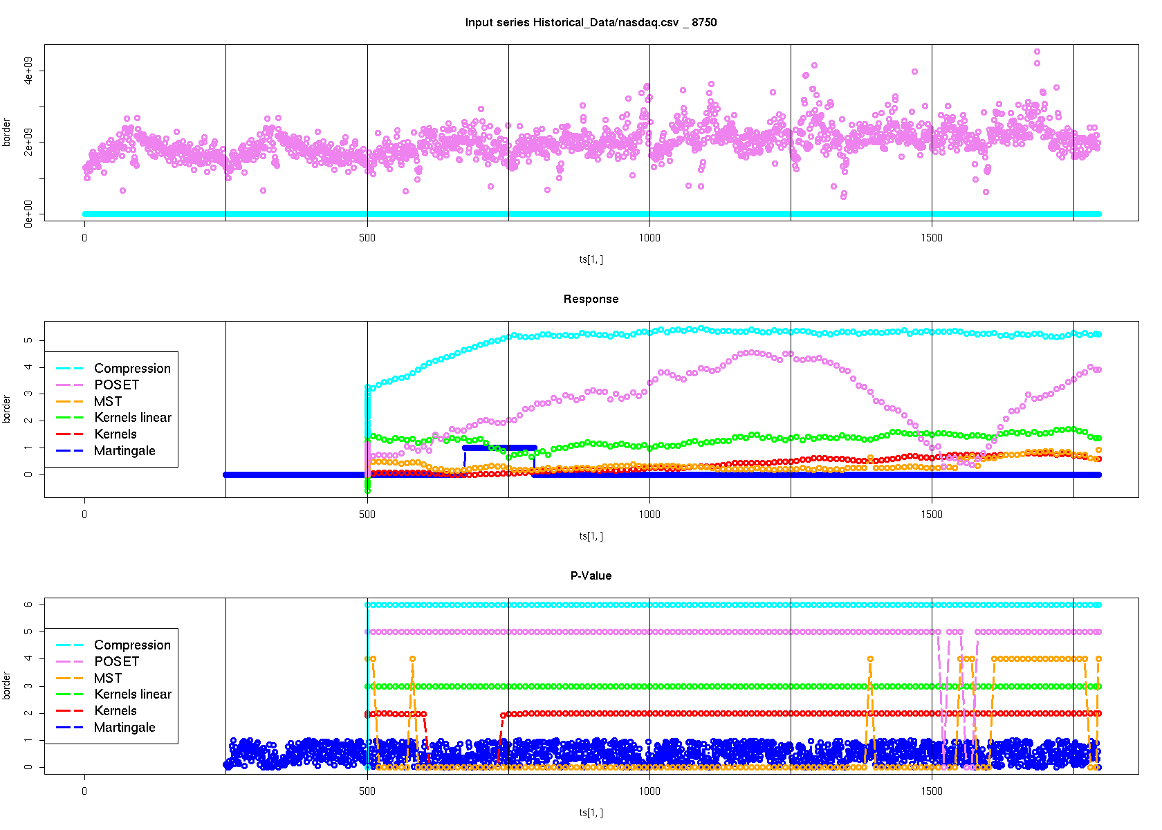
In this section, we consider historical stock quote data as a series generated by a stochastic process. A series of quotes is a 6-dimensional series with the following components: open price, high price, low price, close price, volume, and adjusted price. Each point in the series represents a single trading day (ignoring holidays and weekends), and we consider it a continuous series.
We considered four ticker symbols: YHOO (Yahoo!), AAPL (Apple), GOOG (Google), and NASDAQ (index). The first three provide a historical picture of companies in the technology sector, and the last one is an index, which contains these companies. We are interested in exploring whether a stock’s performance has a repeating pattern, and then whether a year can repeat itself.
In the previous examples, we performed the interval analysis by specifying the window length and and shifted the moving window in steps of size . In this experiment we performed a scan analysis. We consider the full historical series, and use the first year as the reference window and for tuning purposes. The moving window has the same length as , and is shifted by small increments of ten points to scan the series. This results in scanning the series by two-week interval steps. Once the scan is completed, we remove the first year and, repeat the process for the cropped series. In this way, we tested the entire series. Notice that the Martingale method always performs a scan of the series one point at a time.

Our goal is to find similarity in order to prove that there is a repeating pattern or at least identical years. We replace the exact dates in favor of referring to the number of years since the first stock offering was traded. Due to the small number of dimensions, the poset method should provide a reasonable set of similar years. We do not normalize the series in order to take account of inflation or other dollar valuations. Thus, we can identify recession years, when a quote drops to previous values, and recovering years. For example, an index such a NASDAQ is bound to increase during its lifetime as a result of adding new stocks or accounting for the value of the dollar. For such a quote, we are most likely to find only recession years. By contrast, a quote such as AAPL may exhibit periods of growth after a recession.
IXIC NASDAQ. The NASDAQ index presents two pairs of years with similarity that coincide with recessions. We have found one period of no growth between the 24–25-th years and another similar recession between the 45-th and the 50-th years. These two findings indeed match two weak market periods. In fact, the 50-th interval coincides with the 2008 fiscal year. In Figure 16, we present the experimental results.
APPL. We found at least two similar years, both representing a period before growth of the company (9-th and 21-th). In Figure 17, we present the experimental results.
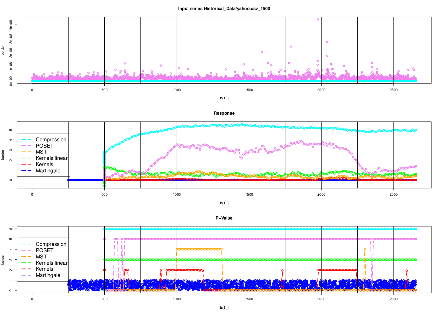
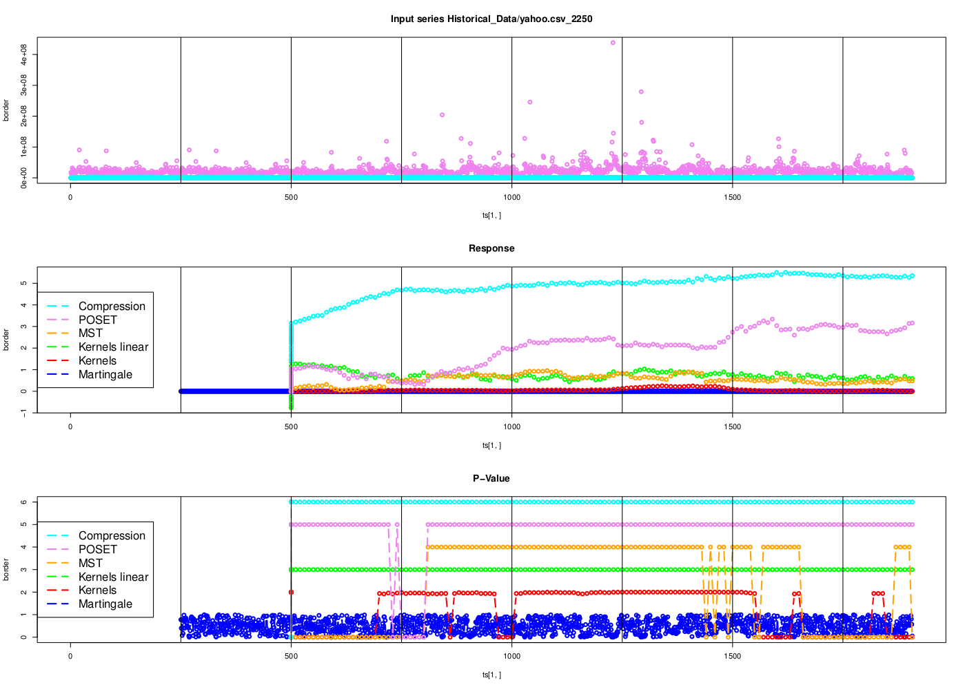
YHOO. We found two similar years. The 6-th and the 14-th years represent a rebound of the quote right after the so called tech bubble and housing bubble burst. The 9-th and the 10-th represent a stable period for the company. We present the results for both these time series in Figure 18.
GOOG. As a result of a constant growth pattern, we were not able to find similar years.
8 Single-Dimensional Experimental Results
In this section, we validate the power of our CDF-based measures and compare with the state of the art methods. The comparison is based upon the performance on single-dimension series. For comparison purpose, the measures are organized into two sets:
-
Standard:
This set consists of the following five measures: Wilcoxon–Mann–Whitney, t–test, Kolmogorov–Smirnov, , and .
-
Extension:
This set consists of the following nine measures: Kullback–Leibler (symmetric), Jin-L, Jensen–Shannon, , Hellinger, Variational, Cramér–von Mises, Minkowsky, and Euclid. Among these methods, the Cramér–von Mises has been previously used in the literature; however, to the best of our knowledge, none of the methods have been used for series in the continuous domain .
We shall show that our extension measures are comparable to the standard measures, and they may be used separately or together. The overall measure will permit a more effective statistical test for series with real values.
8.1 Setup
We apply the standard and extension measures, separately and together, on a set of series. The series are generated by repeating the following process 1000 times:
-
•
The time series is composed by a set of consecutive windows. The number of windows is randomly chosen as . The series is composed of at least two windows and at most twenty.
-
•
The window size is randomly chosen as , without any bias to a particular window size. That is, a series is composed of windows of equal size; where every windows has a minimum size of 100 points and a maximum of 1,000.
-
•
A window with the same distribution as the first window is embedded into the series in randomly.
The goal of the tests is to find in the time series and to reject every other window, by scanning the created series using a moving window . Three types of series are generated to reflect changes in the average, changes in the variance, and changes in both the average and the variance.
Change in Average. Using a normal distribution generator , we determine the reference average and variance . We generated two windows and using either a normal distribution or a uniform distribution . For every other window, we selected at random where , switching its sign with equal probability. Therefore, as increases, the series becomes longer, the tailing window of the series tends to be closer to the reference . Using a 20% disagreement threshold, the system recognized the similarity with a sharp positive pulse, correctly flagging all the other intervals as different.
Change in Variance. We generated two windows and using either a normal distribution or a uniform distribution, as described previously, using and . For every other window, we selected at random where , switching its sign with equal probability. Therefore, as increases, the series becomes longer, the tailing window of the series tends to be closer to the reference . Using a 20% disagreement threshold, the system recognized the similarity with a rather slow positive pulse; however, it also recognized other intervals as similar, resulting in false positives.
Changing Both Average and Variance. We generated two windows and using either a normal distribution or a uniform distribution . For every other window, we selected at random and from . Using a 20% disagreement threshold, the system recognized the similarity with a sharp positive pulse, correctly flagging all the other intervals as different.
For the experiments where we changed only the average or the variance, the test series converged to the reference window. For large enough , the measures would find it harder and harder to distinguish them. Yet, there was only one window in the series that had the same attributes as the reference.
Moving Window. The moving window scans the series. The moves by a fixed size step of 100 epochs/points. Note that 100 is the smallest windows size possible, thus the sliding window is always contained into a classified window with a well defined statistical properties.
Disagreement. We quantified the number of times the system recognized two windows as the same for different level of disagreement (0.1, 0.2, 0.3, 0.4., 0.5., 0.6., 0.7, 0.8, 0.9, 1). That is, with a disagreement of 0.1, two windows are recognized as equal if, at most, 1 out of 10 measures does not say so, while the remaining measures do.
Matching and Found. We define a match as having occurred when the system produces a positive response for two windows and , which we know are equal. The golden standard for matches is 1000, which is equal to the number of windows that were drawn from the same distribution when the series was generated. We define found as having occurred when the system produces a positive response independent of the position in the series, because the sliding window has a fixed step of 100 epochs instead of the effective window size. For example, if , thus the series is composed of widows of size 1,000, there could be one match and 19 founds, because will lie on top of once, but it will overlap with about 19 times.
8.2 Summary Results
We define the number of times an error was committed as . That is, the combination of false positives and false negatives, where false positives are when the system identifies two windows as being equal minus the golden standard, and false negatives are the number of misses made by the system.
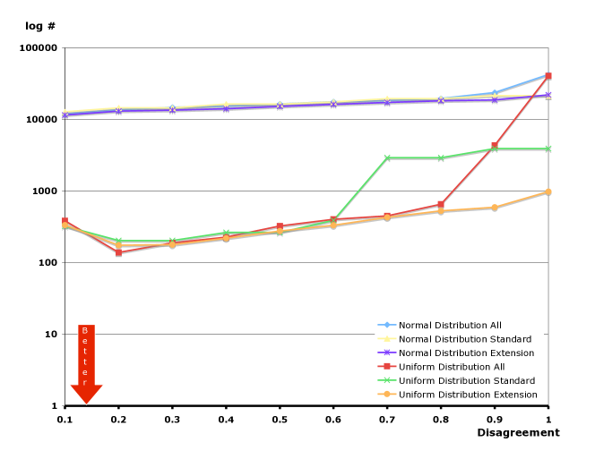
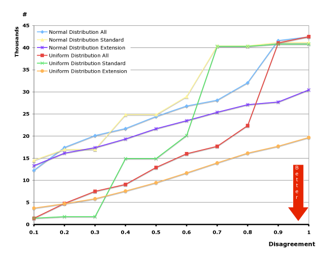
In Figure 19, we present the error for change in average only and change in variance only. Notice that for a change in average only, the combination of both standard and extension measures produces the smallest error, resulting in a Gestalt effect. This effect alone justifies the addition of our methods.
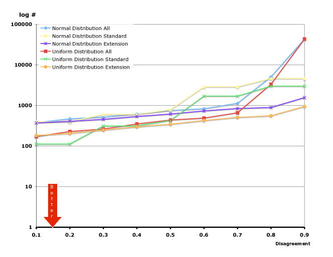
In Figure 20, we present the error for changes in both the average and variance. Notice that the standard approach has a smaller error over the range of 0.1 and 0.2 for uniformly distributed series. However it has the same error as our extension methods for series using normal distributions. Overall, our extensions work well, performing consistently as a function of the disagreement factor.
Note: our new CDF based methods are a simple to deploy and a good addition to the standard measures. As we showed for multidimensional series, we present methods that add on top of the existing methods without replacing them or be overshadowed by them. These methods are a contribution to the field.
8.3 Results for Change in Average
In Figure 21, we show that our extension methods perform better than the standard methods, which means our methods are more sensitive to detecting changes in the average.
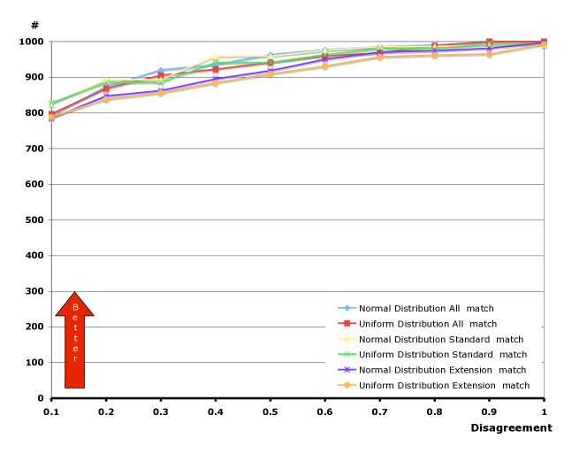
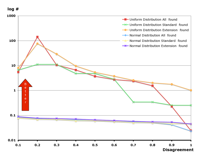
8.4 Results for Change in Variance
In Figure 22, we find that the standard measures offer a more sensitive tool for detecting true similarity (or conversely an anomaly).
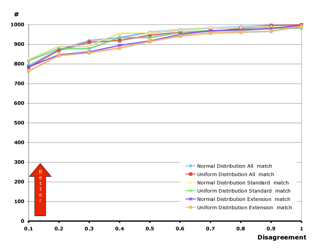
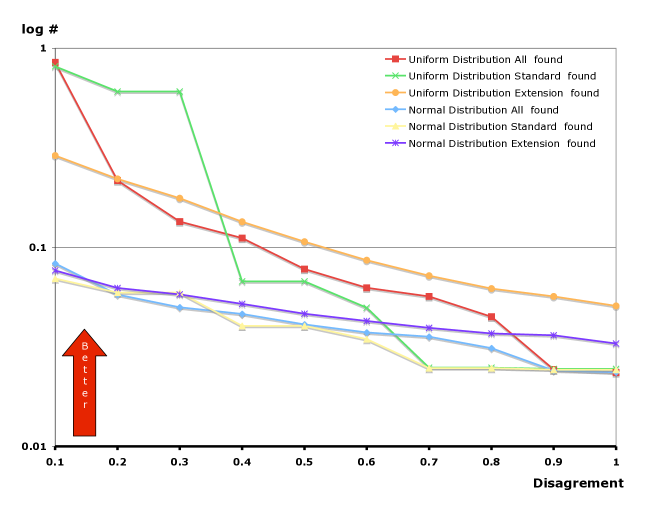
8.5 Results for Change in Average and Variance
In Figure 23, we present the number of perfect matches and the number of found matches by all approaches. The standard methods appear to out-perform the extensions when using the right balance of consensus and disagreement for series built using a uniform distribution. However, our extension methods deliver a predictable and ultimately better performance for inputs drawn from a normal stochastic process.
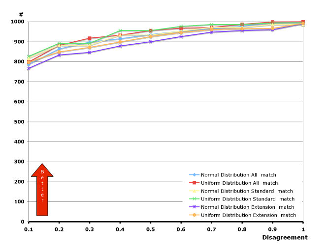
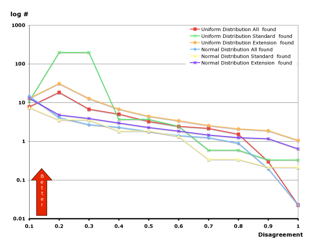
9 Conclusions
We have presented a survey of the different methods for detecting stochastic change in multi-dimensional series. This included a detailed examination of four types of promising methods: Kolmogorov’s information measure, the Martingale measure in conjunction with conformal prediction, kernel methods for the computation of the maximum mean discrepancy measure, and topological-order based methods that are built on the comparison of empirical distribution functions. To complete this work, we proposed new measures for the comparison of empirical distributions previously applied only to single-dimension series, and applied them to multi-dimensional series.
We have shown that each measure is different and exploits different properties of the data. As a result, each measure provides valuable information about the data. Although the measures range in computational complexity, there are measures which are relatively fast, such as the linear kernel method at , the poset-based method and compression method at , and finally the Martingale, kernel, and MST methods at . Furthermore, we show that this variety of methods and their inherent capabilities is also apparent for one–dimensional-series methods, which have a much longer history.
This paper is intended to be a self-contained work that includes a survey of existing methods and an original contribution. The authors would like to emphasize that although this is long standing research field, mature and widely used–applied, it is far from being solved having a never ending, always interesting research depth and still offering surprising new results.
The authors would like to thank: Prof. Daniel Kifer of the Department of Computer Science and Engineering Penn State University for the discussions about single-dimension series stochastic distances, Prof. Vladimir Vovk of the Department of Computer Science University of London for the discussions about conformal prediction, Prof. Paul Vitanyi of University of Amsterdam and Rudi Cilibrasi Ph.D. for the discussions about compression distance, Alexander Smola Ph.D. principal research scientist Yahoo! and Prof. Australian National University for discussions about kernel methods, Arun Kejariwal Ph.D. (now at Netflix) and Rosario Cammarota (Ph.D. Candidate ICS UCI) for the discussions and data about the SPEC hardware/software performance.
The authors thank Yahoo! Inc. for the resources, the support given, and the understanding for this research that spanned about 4 years. The final result of this work is a stochastic library that the authors will provide to interested affiliations.
References
- Ali and Silvey (1966) Ali, S. and Silvey, S. 1966. A general class of coefficients of divergence of one distribution from another. Journal of the Royal Statistical Society. Series B 28, 1, 131–142.
- Anderson (1962) Anderson, T. 1962. On the distribution of the two-sample Cramer–von Mises criterion. Annals of Mathematics Statistics 33, 3, 1148–1159.
- Aronszajn (1950) Aronszajn, N. 1950. Theory of reproducing kernels. Transactions of the American Mathematical Society 68, 3, 337–404.
- Batchelor (1978) Batchelor, B. 1978. Pattern Recognition: Idea and Practice. New York: Plenum Press.
- Bennett et al. (1998) Bennett, C. H., Gács, P., Li, M., Vitányi, P. M. B., and Zurek, W. H. 1998. Information distance. IEEE Transactions on Information Theory 44, 4, 1407–1423.
- Bhattacharyya (1943) Bhattacharyya, A. 1943. On a measure of divergence between two statistical populations defined by probability distributions. Bulletin Calcutta of Mathematics Society 35, 99–109.
- Biau and Gyorfi (2005) Biau, G. and Gyorfi, L. 2005. On the asymptotic properties of a nonparametric l1-test statistic of homogeneity. IEEE Transactions on Information Theory 51, 11, 3965 – 3973.
- Bickel et al. (2006) Bickel, P., Ritov, Y., and Stoker, T. 2006. Tailor-made tests for goodness-of-fit to semiparametric hypotheses. Annals Of Statistics 34, 2, 721–741.
- Bickel (1969) Bickel, P. J. 1969. A distribution free version of the smirnov two sample test in the p-variate case. The Annals of Mathematical Statistics 40, 1, 1–23.
- Borgwardt et al. (2006) Borgwardt, K. M., Gretton, A., Rasch, M. J., Kriegel, H.-P., Schölkopf, B., and Smola, A. J. 2006. Integrating structured biological data by kernel maximum mean discrepancy. In ISMB (Supplement of Bioinformatics). 49–57.
- Cammarota et al. (2011) Cammarota, R., Kejariwal, A., D’Alberto, P., Panigrahi, S., Veidenbaum, A., and A.Nicolau. 2011. Pruning hardaware evaluation space via causality-driven application similarity analysis. In ACM International Conference on Computer Frontiers.
- Chakrabarti et al. (1998) Chakrabarti, S., Sarawagi, S., and Dom, B. 1998. Mining surprising patterns using temporal description length. In VLDB ’98: Proceedings of the 24rd International Conference on Very Large Data Bases. Morgan Kaufmann Publishers Inc., San Francisco, CA, USA, 606–617.
- Chernoff (1952) Chernoff, H. 1952. A measure of asymptotic efficiency for tests of a hypothesis based on the sum of observations. The Annals of Mathematical Statistics 23, 4, 493–507.
- Cilibrasi and Vitányi (2005) Cilibrasi, R. and Vitányi, P. M. B. 2005. Clustering by compression. IEEE Transactions on Information Theory 51, 4, 1523–1545.
- D’Alberto and Dasdan (2009) D’Alberto, P. and Dasdan, A. 2009. Non-parametric information-theoretic measures of one-dimensional distribution functions from continuous time series. In Proceedings of the Ninth SIAM International Conference on Data Mining, SIAM, Ed. Sparks, NV.
- Daskalakis et al. (2009) Daskalakis, C., Karp, R. M., Mossel, E., Riesenfeld, S., and Verbin, E. 2009. Sorting and selection in posets. In SODA ’09: Proceedings of the twentieth Annual ACM-SIAM Symposium on Discrete Algorithms. Society for Industrial and Applied Mathematics, Philadelphia, PA, USA, 392–401.
- Dasu et al. (2006) Dasu, T., Krishnan, S., Venkatasubramanian, S., and Yi, K. 2006. An information-theoretic approach to detecting changes in multi-dimensional data streams. In In Proc. Symp. on the Interface of Statistics, Computing Science, and Applications.
- Diday (1974) Diday, E. 1974. Recent progress in distance and similarity measures in pattern recognition. In Second International Joint Conference on Pattern Recognition. 534–539.
- Einmahl and Khmaladze (2001) Einmahl, J. and Khmaladze, E. 2001. The two-sample problem in rm and measure-valued martingales. Open access publications from tilburg university, Tilburg University.
- Faigle and Turán (1988) Faigle, U. and Turán, G. 1988. Sorting and recognition problems for ordered sets. SIAM Journal on Computing 17, 1, 100–113.
- Feller (1948) Feller, W. 1948. On the kolmogorov-smirnov limit theorems for empirical distributions. The Annals of Mathematical Statistics 19, 2, 177–189.
- Feller (1971) Feller, W. 1971. An Introduction to Probability Theory and its Applications 2 Ed. Vol. 2. John Wiley & Sons.
- Frank and Asuncion (2010) Frank, A. and Asuncion, A. 2010. UCI machine learning repository.
- Friedman and Rafsky (1979) Friedman, J. and Rafsky, L. 1979. Multivariate generalizations of the wald-wolfowitz and smirnov two-sample tests. The Annals of Statistics 7, 4, 697–717.
- Fuglede and Topsoe (2004) Fuglede, B. and Topsoe, F. 2004. Jensen-Shannon divergence and Hilbert space embedding. In IEEE International Symposium on Information Theory. 31–31.
- Glaz et al. (2001) Glaz, J., Naus, J., and Walleenstein, S. 2001. Scan Statistics. Springer series in statistics. Springer-Verlag.
- Golub and Loan (1996) Golub, G. and Loan, C. V. 1996. Matrix Computations 3 Ed. The Johns Hopkins Univ. Press (Oct. 15, 1996).
- Gretton et al. (2006) Gretton, A., Borgwardt, K. M., Rasch, M. J., Schölkopf, B., and Smola, A. J. 2006. A kernel method for the two-sample-problem. In NIPS, B. Schölkopf, J. C. Platt, and T. Hoffman, Eds. MIT Press, 513–520.
- Gretton et al. (2008) Gretton, A., Borgwardt, K. M., Rasch, M. J., Schölkopf, B., and Smola, A. J. 2008. A kernel method for the two-sample-problem. Extended Version of the NIPS2006.
- Gretton et al. (2007) Gretton, A., Fukumizu, K., Teo, C. H., Song, L., Schölkopf, B., and Smola, A. J. 2007. A kernel statistical test of independence. In NIPS, J. C. Platt, D. Koller, Y. Singer, and S. T. Roweis, Eds. MIT Press.
- Hahn (1912) Hahn, H. 1912. Über die integrale des herrn Hellinger und die orthogonalinvarianten der quadratischen formen von unendlich vielen veränderlichen. Journal Monatshefte für Mathematik 23, 1, 161–224.
- Hall and Tajvidi (2002) Hall, P. and Tajvidi, N. 2002. Permutation tests for equality of distributions in high-dimensional settings. Biometrika 89, 2, 359–374.
- Harel (1993) Harel, A. 1993. Random walk and the area below its path. Mathematics of Operations Research 18, 3, 566–577.
- Henning (2006) Henning, J. L. 2006. Spec cpu2006 benchmark descriptions. SIGARCH Comput. Archit. News 34, 4, 1–17.
- Ho (2005) Ho, S.-S. 2005. A martingale framework for concept change detection in time-varying data streams. In Proceedings International Conference on Machine Learning (ICML). Bonn, Germany.
- Ho and Wechsler (2005) Ho, S.-S. and Wechsler, H. 2005. On the detection of concept change in time-varying data streams by testing exchangeability. In Proceedings Conference on Uncertainty in Artificial Intelligence (UAI). Edinburgh, Scotland.
- Ho and Wechsler (2010) Ho, S.-S. and Wechsler, H. 2010. A martingale framework for detecting changes in data streams by testing exchangeability. IEEE Transactions on Pattern Analysis and Machine Intelligence 99, PrePrints.
- Hope (1968) Hope, A. A. 1968. A simplified Monte Carlo significance test procedure. Journal of the Royal Statistical Society. Series B (Methodological) 30, 3, 582–598.
- Horton and Nakai (1996) Horton, P. and Nakai, K. 1996. A probabilistic classification system for predicting the cellular localization sites of proteins. In Proceedings of the Fourth International Conference on Intelligent Systems for Molecular Biology. AAAI Press, 109–115.
- Jensen (1906) Jensen, J. 1906. Sur les fonctions convexes et les in galit s entre les valeurs moyennes. Acta Mathematique 30, 175–193.
- (41) Johnson, D. and Sinanovic, S. Symmetrizing the Kullback–Leibler distance.
- Jones and Furnas (1987) Jones, W. and Furnas, G. 1987. Pictures of relevance: A geometric analysis of similarity measures. Journal of American Society for Information Science 38, 6, 420–442.
- Kagan (1963) Kagan, A. 1963. Towards the theory of Fisher’s amount of information. Doklady Akademii nauk SSSR. 151, 277–278. (in Russian).
- Kailath (1967) Kailath, T. 1967. The divergence and Bhattacharyya distance measures in signal selection. IEEE Transactions on Communications 15, 1, 52–60.
- Kendall (1991) Kendall, D. 1991. Andrei Nikolaevich Kolmogorov. 25 april 1903-20 october 1987. Biographical Memoirs of Fellows of the Royal Society, 37, 301–319.
- Keogh et al. (2004) Keogh, E., Lonardi, S., and Ratanamahatana, C. A. 2004. Towards parameter-free data mining. In KDD ’04: Proceedings of the tenth ACM SIGKDD international conference on Knowledge discovery and data mining. ACM, New York, NY, USA, 206–215.
- Kifer et al. (2004) Kifer, D., Ben-David, S., and Gehrke, J. 2004. Detecting change in data streams. In Proceedings International Conference on Very Large Data Bases (VLDB). Morgan Kaufmann, Elsevier, Toronto, Canada, 180–191.
- Kim and Foutz (1987) Kim, K.-K. and Foutz, R. V. 1987. Tests for the multivariate two-sample problem based on empirical probability measures. The Canadian Journal of Statistic 15, 1, 41–51.
- Kolmogorov (1933) Kolmogorov, A. 1933. Sulla determinazione empririca di una legge di distribuzione. Giornale Istituzioni Italiane Attuari 4.
- Kolmogorov and Uspenskii (1987) Kolmogorov, A. N. and Uspenskii, V. A. 1987. Algorithms and randomness. Theory of Probability and its Applications 32, 3, 389–412.
- Kullback and Leibler (1951) Kullback, S. and Leibler, R. A. 1951. On information and sufficiency. The Annals of Mathematical Statistics 22, 1, 79–86.
- Kulldorf (1997) Kulldorf, M. 1997. A spatial scan statistic. Communications In Statistics Theory And Methods 26, 6, 1481–1496.
- Kulldorff et al. (2007) Kulldorff, M., Mostashari, F., Duczmal, L., Yih, K., Kleinman, K., and Platt, R. 2007. Multivariate spatial scan statistics for disease surveillance. Statistics in Medicine 26, 1824–1833.
- Lee (1999) Lee, L. 1999. Measures of distributional similarity. In Proceedings of the 37th annual meeting of the Association for Computational Linguistics on Computational Linguistics. Morristown, NJ, USA, 25–32.
- Li et al. (2004) Li, M., Chen, X., Li, X., Ma, B., and Vitányi, P. M. B. 2004. The similarity metric. IEEE Transactions on Information Theory 50, 12, 3250–3264.
- Lin (1991) Lin, J. 1991. Divergence measures based on the Shannon entropy. IEEE Transactions on Information Theory 37, 1, 145–151.
- Magel and Wibowo (1997) Magel, R. C. and Wibowo, S. H. 1997. Comparing the powers of the wald-wolfowitz and kolmogorov-smirnov tests. Biometrical Journal 39, 6, 665–675.
- Mann and Whitney (1947) Mann, H. B. and Whitney, D. R. 1947. On a test of whether one of two random variables is stochastically larger than the other. The Annals of Mathematical Statistics 18, 1, 50–60.
- Martin-Lof (1969) Martin-Lof, P. 1969. Algorithms and randomness. Review of the International Statistical Institute 37, 3, 265–272.
- Meintanis and Iliopoulos (2008) Meintanis, S. G. and Iliopoulos, G. 2008. Fourier methods for testing multivariate independence. Computational Statistics and Data Analysis 52, 4, 1884–1895.
- Melucci (2007) Melucci, M. 2007. On rank correlation in information retrieval evaluation. SIGIR Forum 41, 1, 18–33.
- Müller (1997) Müller, A. 1997. Integral probability metrics and their generating classes of functions. Advances in Applied Probability 29, 2, 429–443.
- Nash et al. (1994) Nash, W. J., Sellers, T. L., Cawthorn, S. R. T. A. J., and Ford, W. B. 1994. The population biology of abalone (haliotis species) in tasmania i. blacklip abalone (h. rubra) from the north coast and islands of bass strait. Tech. Rep. 48, Sea Fisheries Division.
- Pinsker (1960) Pinsker, M. 1960. Information and information stability of random variables and processes. Probl. Peredachi Inf. 7.
- Schölkopf and Smola (2002) Schölkopf, B. and Smola, A. 2002. Learning with Kernels. MIT Press.
- Shafer and Vovk (2008) Shafer, G. and Vovk, V. 2008. A tutorial on conformal prediction. J. Mach. Learn. Res. 9, 371–421.
- Shannon (1948) Shannon, C. 1948. A mathematical theory of communication. The Bell System Technical Journal 27, 379–423 and 623–656.
- Shivakumar and García-Molina (1995) Shivakumar, N. and García-Molina, H. 1995. SCAM: A copy detection mechanism for digital documents. In Proceedings 2nd Conference on the Theory and Practice of Digital Libraries.
- Siegel (1959) Siegel, S. 1959. Nonparametric statistics, for the behavioral sciences. Series in Psychology. McGraw-Hill book company.
- Song et al. (2007) Song, X., Wu, M., Jermaine, C., and Ranka, S. 2007. Statistical change detection for multi-dimensional data. In KDD ’07: Proceedings of the 13th ACM SIGKDD international conference on Knowledge discovery and data mining. ACM, New York, NY, USA, 667–676.
- Sriperumbudur et al. (2009) Sriperumbudur, B. K., Gretton, A., Fukumizu, K., Lanckriet, G. R. G., and Schölkopf, B. 2009. A note on integral probability metrics and -divergences. CoRR abs/0901.2698.
- Street et al. (1993) Street, W., Wolberg, W., and Mangasarian, O. 1993. Nuclear feature extraction for breast tumor diagnosis. In IS&T/SPIE 1993 International Symposium on Electronic Imaging: Science and Technology. Vol. 1905. San Jose, CA, 861–870.
- Takács (1991) Takács, L. 1991. A bernoulli excursion and its various applications. Advances in Applied Probability 23, 3, 557–585.
- Taneja and Kumar (2004) Taneja, I. J. and Kumar, P. 2004. Relative information of type s, Csiszár’s f-divergence, and information inequalities. Information Sciences 166, 105–125.
- Terwijn et al. (2010) Terwijn, S. A., Torenvliet, L., and Vitányi, P. M. 2010. Nonapproximability of the normalized information distance. Journal of Computer and System Sciences In Press, Corrected Proof, –.
- Tsanas et al. (2010) Tsanas, A., Little, M., McSharry, P., and Ramig, L. 2010. Accurate telemonitoring of parkinson.s disease progression by non-invasive speech tests. Biomedical Engineering, IEEE Transactions on.
- Vajda (1972) Vajda, I. 1972. On the -divergence and singularity of probability measures. Journal Periodica Mathematica Hungarica 2, 1–4, 223–234.
- Vovk (1993) Vovk, V. 1993. A logic of probability, with application to the foundations of statistics. Journal of the Royal Statistics Society 55, 2, 317–351.
- Vovk et al. (2005) Vovk, V., Gammerman, A., and Shafer, G. 2005. Vovk, Vladimir, Gammerman, Alex, Shafer, Glenn. Springer.
- Vovk et al. (2003) Vovk, V., Nouretdinov, I., and Gammerman, A. 2003. Testing exchangeability on-line. In Proceedings International Conference on Machine Learning (ICML).
- Wald (1947) Wald, A. 1947. Sequential Analysis. Dover Publications Inc, N.Y.
- Wang et al. (2005) Wang, Q., Kulkarni, S. R., and Verd , S. 2005. Divergence estimation of continuous distributions based on data-dependent partitions. IEEE Transactions on Information Theory 51, 9, 3064 – 3074.
- Wang et al. (1992) Wang, Z., Wong, S., and Yao, Y. 1992. An analysis of vector space models based on computational geometry. In Proceedings International Conference on Research and Development in Information Retrieval (SIGIR). ACM, New York, NY, USA, 152–160.
- Wilcoxon (1945) Wilcoxon, F. 1945. Individual comparisons by ranking methods. Biometrics Bulletin 1, 80–83.
- Wilson and Martinez (1997) Wilson, D. R. and Martinez, T. R. 1997. Improved heterogeneous distance functions. Journal of Artificial Intelligence Research 6, 1–34.
- Zhang et al. (2008) Zhang, X., Song, L., Gretton, A., and Smola, A. J. 2008. Kernel measures of independence for non-iid data. In NIPS, D. Koller, D. Schuurmans, Y. Bengio, and L. Bottou, Eds. MIT Press, 1937–1944.
10 Review 1
This paper reviews 4 different families of non-parametric methods to
 detect anomalies in time series, more specifically a change in the
 distribution of points which are sampled sequentially and
 independently. This task is usually referred to as change point
 detection. Of all 4 techniques, part of the 1st one and the 4th one
 are original contributions. The 4th method aims at comparing two
 sub-series R and W by estimating their respective Cumulative Density
 Functions (CDF) F_R and F_W, and then computing many distances
 D(F_R,F_W) to evaluate how dissimilar they are. A change is detected
 whenever a "quorum" of alarms/flags are raised, that is a sufficient
 number of distances go above a given threshold. These distances are
 presented in Section 4. Section 5 follows with experimental results
 with 3 simulated sets of time series (toy data, classification data,
 applications calls) and 1 real-life dataset (quote history for 4
 stocks).

Regardless of the interest of its contribution, I think the paper has
 many problems with its current form. I think this paper would have
 greatly benefitted from further polishing, rewriting and
 proofreading. In particular, I have the feeling that the authors have
 settled for a paper structure and notations that could looks sloppy,
 which contrasts with their self advocated goal of proposing new tools
 but also proposing a unified framework (footnote 1, p.2 or bottom of
 p.2). Here are few items that illustrate these impressions, and which
 the authors need to take care:

- bibliographic pointers are most often given at the end of the
 sections (e.g middle of p.15, bottom of p.22, p.30 etc.) instead of
 being provided right next to the introduction of important concepts
 as is common practice in ML. This makes it particularly difficult to
 understand on which literature the methods which are presented here
 are based upon.  Nothing is more important for a reader interested in
 a review paper than being able to frequently check references exactly
 at the moment when they are introduced, with page and section
 numbers.

- Overall, mathematical statements and notations are loose and lack
 clarity. Mathematical terms are overloaded. Overall, there are very
 few equations and a lot of text, which makes it difficult to check or
 understand exactly the authors’ claims. Here are a few examples: **
 The title "Non-parametric methods applied to time series comparison"
 is not well chosen. The authors only handle time series of
 independent measurements. This is a *very* restrictive case when
 studying time series, which is known as change point detection. I
 would suggest something along the lines of "Non-parametric methods
 for Change Point Detection"

** The crux of the problem, is not well posed. In particular, the
 authors use the following sentence (p.5, before 2.2) to introduce
 change point detection: "A change occurs any time that W is different
 from R". What do you mean by "different"? if taken literally, then I
 guess that unless a series is constant there are always changes. Do
 the authors mean in distribution? Then why are not any of the
 standard definitions of change given here? The authors may want to
 refer to "Detection of Abrupt Changes: Theory and Application",
 M. Basseville, I. Nikiforov for such definitions.

**Since the authors kick out their methodological section without
 actually defining the problem, it is extremely difficult for the
 reader to understand their perspective. The introduction of Section 3
 is, for instance, quite disorganized. For instance, I do not
 understand what the authors mean by "What distinguishes our work from
 others is the focus on the computational aspects of implementing each
 method in a context of a set of statistical tools" nor think that the
 "we feel that we have taken the works of Bickel [8] and
 Friedman-Rafsky [24] and succeeded in extracting the common features"
 is particularly convincing, specially in the introduction of this
 section.

** Section 3.3 is the most problematic, mathematically speaking, and
 has to be entirely rewritten by following standard conventions,
 e.g. being careful with the notation for f, the function, and f(x), a
 number. Non-exhaustive list of examples

--- "Assume that F is a Hilbert space defined in E; that is f(x) with
 x \in E" ??

--- "First, for every fixed y=y0, then K(x,y0)\in F". K(x,y0) is a
 number, not a function. "x -> K(x,y0)" would be a function, or
 K(.,y0) using the dot notation.

--- "found the existence of a mapping phi(x)", again, the mapping is
 phi or x -> phi(x) but not phi(x).  Since this paragraph is really
 standard, it is annoying to stumble every other line on these
 confusions.


** The main contribution of the authors, Section 3.4, is extremely
 difficult to parse, with no formal definition/proposition/algorithm
 box nor figure. The structure is very sloppy here: there are 7
 (non-numbered) remarks over 4 pages which are provided one after the
 other with very little context. Since this should be the strongest /
 best motivated part of the paper, this section is disappointing.

** Results in the experimental section are not well presented. The
 axis and/or legends of figures 2,3, 5, 8, 9, 10, 11, 12, 13 of
 section 5 are impossible to read, which is to say most figures are
 hardly of any use at this point. When readable, most of the times the
 text on the axis is not clear (e.g. "Result[[XVAL]][x]")

** minor issues which break the reading flow:

--- the authors use the word "measure" without a formal explanation
 from the beginning of section 3. I think what the authors call a
 measure is widely known as a divergence, or possibly a dissimilarity
 or a distance in some cases. A measure is usually a map from a
 sigma-algebra to real numbers that satisfies sigma-additivity, as
 defined in "measure theory". The words "similarity measure" is
 sometimes used to denote a similarity, but "measure" in itself is not
 used as a synonym of divergence in the machine learning
 literature. The authors also use "measure" for both a distance or a
 similarities (or a kernel actually), e.g. p.36 Bhattacharyya section.

--- Why separate references to seminal works of Jensen [40] and
 Shannon [67] to mention the Jensen-Shannon divergence? I do not think
 either of these authors actually proposed it, and certainly not in
 either of these papers.

--- The statement that follows, on "commonality" of phi-divergences
 and RKHS as illustrated by the "embedability" of the Jensen-Shannon
 divergence is enigmatic. The Jensen-Shannon divergence is a negative
 definite distance between probability measures.  It can be shown that
 probability measures can thus be embedded in a Hilbert space where
 the regular norm of that RKHS coincides with the distance,
 i.e. JS(p,q)= || phi(p) - phi(q) ||_K . What is the relation with
 using phi-divergences between measures mapped in a RKHS (induced by
 any kernel) as advocated by [71]?

--- in p.5 the authors distinguish epochs and timestamps in a not so
 clear way but then resolve to only focus on timestamps in the
 paper. this discussion is not needed.

--- p.11 section 3.1.2: transducers are introduced as f_A, but the
 authors never use that notation again. a transducer is defined as a
 function (S^*) -> [0,1], but the authors use a conditional form to
 define it right below, that takes at least 2 parameters - m and N -
 that do not fit your definition of a function from (S^*).

--- p.13 section 3.1.3 has three properties. I am not sure what the
 authors mean by "Property".

--- p.15 the introduction of section 3.2 needs to be rewritten, and
 key notations like Y properly defined.

--- is the normalized compression distance a distance (definite,
 triangle inequality)?

--- the definition of completeness and cauchy sequences at the bottom
 of p. 18 is wrong.

--- p.20 footnote 3: referring to "choosing a kernel" as an "art" is
 not particularly convincing, given that there have been hundreds of
 papers that try to select kernels adaptively (MKL) and a few more for
 the MMS case in particular.

--- I do not understand the motivation of the authors to refer to "red
 points" and "white points" without illustrating their ideas with a
 figure.

--- p.32, bottom: the definition of the 0 norm is pretty much
 standardized in the literature, and is the natural limit of the p
 norm when p goes to 0. I have never seen it defined as the algebraic
 sum of all terms of a vector as proposed by the authors (which would
 violate the fact that a norm needs to be non-negative anyway).

--- p.34 the authors should use italics more sparingly in this
 section, specially on subjective calls like "*more* trustworthy"
 etc..

--- p.36 Hellinger: "component-wise comparison is less biased", biased
 in what sense? the statement "components near the extremes (0 or 1)
 are moved closer to 1/2 [by the square root]" is wrong.

--- section 4.1.3 mentions a few other "measures" but only quotes
 Wilcoxon-Mann-Whitney.

Now, on the content itself. First, I have to say that is has been
 relatively difficult for me to read the paper because of the problems
 highlighted above. Yet, on the content itself, I have been puzzled by
 the following points:

##### no reference to classics in the change point detection
 literature

"Detection of Abrupt Changes: Theory and Application", M. Basseville,
 I. Nikiforov

nor on the recent literature on change point detection with kernels,

"Kernel Change-point Analysis", Harchaoui, Bach, Moulines, NIPS 2008

which is, in the context of this paper, more relevant that the MMS
 family of papers [71 etc.], which is a more general tool. The
 reference above discusses specifically the problem considered by the
 authors. Multiple change points have also been considered for
 instance.  "Fast detection of multiple change-points shared by many
 signals using group LARS" Jean-Philippe Vert and Kevin Bleakley
 . NIPS 2010.


##### I do not understand section 4. Why apply divergences that have
 been explicitly designed for probability measures (or probability
 densities) to CDF’s? The authors mention "In this spirit, we can
 extend the measures commonly used for vectors [...] and apply them to
 CDF’s as inputs". I may have missed some additional motivation, but
 at this point the whole idea behind this section does not make sense,
 looks like a hack, and is not supported by any theory in statistics,
 information theory, or information geometry ( e.g. "Methods of
 Information Geometry" Amari Nagaoka).

##### Inadequacy of the datasets. None of the experiments is truly
 convincing for a machine learning application:

-- The experiments with stocks dataset makes very little sense from a
 financial perspective.  No one in the financial industry studies
 stock prices as i.i.d. datasets.  Financial econometrics is the
 discipline that studies financial time series. What do you mean by
 "For example an index such a(sic) Nasdaq is bound to increase during
 its lifetime as a result of adding new stocks". indices are simply
 reweighted when they contain new stocks, not increased.

-- Using (low dimensional) classification datasets to generate time
 series is a nice toy example but not really convincing.

-- The hardware/software application would deserve more information
 and quantitative (dimensions, sample size etc..) description of the
 dataset.

##### The techniques that are proposed (section 3.4) do not work with
 high dimensional data, because of the need for constructing a partial
 order to estimate CDF’s. Isn’t high dimensions one of the most
 obvious challenges in machine learning today?

To summarize, I think the authors need to spend considerably more time
 on this paper to make it fit for a submission. At the moment the
 contribution (3.4) is poorly presented, one of the key ideas (using
 divergences for probability densities directly on CDF’s) makes no
 sense in my opinion, the experimental section needs significant
 rewriting and the datasets are not particularly interesting nor
 relevant to the problem.
11 Review 2
A Review on Non-parametric Methods Applied to Series Comparison.


Contributions of the paper: The paper contains a comprehensive survey
 about non-parametric methods applied to series comparison, and two
 new non-parametric cumulative distribution function comparison
 methods, which are extensions of the work of Bickel [8] and
 Friedman-Rafksy [24].

The papers studies very interesting problems. In my opinion, however,
 the presentation needs considerable improvement before the paper can
 be published. I am especially worried about the technical details;
 the mathematical notations are confusing sometimes, and at many
 places the authors used verbose sentences instead of concise
 mathematical expressions.

The authors intended to write a self-contained review, but
 unfortunately I do not think that readers who are not familiar with
 the topic can fully understand the discussed ideas because the
 mathematical details are not presented with enough care. At many
 places in the paper the explanations are simply vague but verbose
 sentences instead of precisely formulated mathematical expressions.


It is not clear in the paper what those conditions are when the
 discussed methods can be used. Many of the methods in the paper are
 developed only for i.i.d. series, but the authors use them for more
 complex time series without discussing these issues.

My detailed comments are below.

Section 2.2. Examples of Series and Change: In some of these examples
 I would explain the roles of the mathematical terms introduced in
 Section 2.1 such as s_i, x_i, y_i, S, R, W, etc. Currently, the
 mathematical expressions are defined in section 2.1, and examples are
 given in Section 2.2, but Section 2.2 does not use the notations
 introduced in Section 2.1.

Section 3.

I found it very confusing that the authors talk about ?methods for
 multidimensional series? and later they talk about processes, while
 clearly many of the papers cited here are applicable only for
 i.i.d. series of random variables, but they cannot be used for more
 general time series and stochastic processes. Section 3.1 talks only
 about i.i.d. sequences. Section 3.2 is about Kolomogorov?s
 information and discusses general series again.  The author should
 help the readers and explain which tools can be used for
 i.i.d. series only, and how they are going to use these methods for
 more general series, e.g. stock prices.

The are a couple of other nonparametric divergence estimators that the
 authors might want to cite:

?A Nearest-Neighbor Approach to Estimating Divergence between
 Continuous Random Vectors, Qing Wang, Sanjeev R. Kulkarni, Sergio
 Verdu, IEEE International Symposium on Information Theory (ISIT),
 2006.?

?Estimating divergence functionals and the likelihood ratio by convex
 risk minimization. X. Nguyen, M. J. Wainwright and M. I. Jordan. IEEE
 Transactions on Information Theory, 56, 5847-5861, 2010.?


?On the Estimation of alpha-divergences, B. Poczos and J. Schneider,
 International Conference on AI and Statistics (AISTATS), JMLR
 Workshop and Conference Proceedings (15), 609-617,2011.?

Please cite the PhD thesis of Bharath K Sriperumbudur too:
 ?Reproducing kernel space embeddings and metrics on probability
 measures B. K. Sriperumbudur Ph. D. Dissertation, UC San Diego,
 2010?. This work contains many important and interesting results on
 RKHS based divergences estimators.


Page 11: Could you provide a specific example for A_j?

Page 12: ?Although we have implemented a few transducers?. Which ones?

Page 13, Equation 3.5: Please do not use * for multiplication in
 equations (just simply omit the ?*?). Similarly fix this problem in
 the other equations of the paper.

Page 13: Please define p_i again, or reference where it has been
 defined earlier.

Page 13: Section 3.1.3 is called Martingale methods, but it is not
 explained why and which random variables form a martingale.

Page 15: I do not like that authors simple list references at the end
 of sections instead of citing them in the sections where the results
 are used.

Page 15: Please cite those papers where ?similarity metric?,
 ?universal nature of the measure?, ?the algorithmic information
 distance?, and the ?information distance? have been introduced.

Section 3.2, Normalized Compression Distance: The notations should be
 improved here. For example, it is not explained formally with
 mathematical terms what this sentence means: ?y can be described by a
 chain of descriptions xs?.


Page 18: I could not find where the bound M has been defined.

Page 19: <,> is not a vector norm; it is a square of the vector norm
 <,>^{1/2}.

Page 19: The notation needs to be revised: For example, technically
 this sentence does not make sense, although it is clear what the
 authors wanted to write: ?Assume that $\mathcal{F}$ is a Hilbert
 space defined in $E$; that is, f(x) with $x \in E$.? Please change
 this sentence to something like ?Let $\mathcal{F}=\{f: E\to \Real\}$
 be a Hilbert space?.

Furthermore, $K$ kernel has not been defined, and $K(x,y_0)\in
 \mathcal{F}$ is not true either, since $K(x,y_0)\in \Real$! Please
 use the $K(\cdot,y_0)\in \mathcal{F}$ notation instead.

Similarly, use $f(y)=<f,K(\cdot,y)>$ instead of $f(y)=<f(x),K(x,y)>$!
  The not precise enough notation is especially confusing for the
 feature functions phi, because here $\phi(x)(\cdot)\in
 \mathcal{F}$. Therefore, $f(x)=<f,phi(x)>$ is correct, but
 $phi(x)=<phi(y),K(y,x)>$ is not correct. Please use
 $phi(x)=<phi,K(\cdot,x)>$ instead.

Page 19: ?This is a single dimensional space?. What is a single
 dimensional space?

Page 20: E.q. 3.15: Note that ?U? stands for the U statistic and for
 the unbiased estimation of MMD^2. Sometimes capital U, sometimes
 lower case u is used for the same quantity. Please fix it.

Page 21: ?matrix $\Sigma$ is a semi-definite ...? -> ?matrix $\Sigma$
 is a positive semi-definite ...?

Page 22: Section 3.3.2. Please emphasize more that MMD has been
 defined only for i.i.d. series.

Page 23: The description of the statistical tests is very confusing
 because the authors use the same notations for both the empirical and
 the true cumulative distribution functions! So from the text
 currently it seems the authors want to build a test to decide if the
 two empirical distribution functions are the same, which does not
 make sense, since the empirical distribution functions can be
 computed. The goal of the tests should be to decide if the true
 distribution functions are the same or not.

Page 25: A figure would help to show the meaning of $vdash$ and
 $dashv$.

Page 26: $\vdash_i=\min x_i$, $\dashv_i=\max x_i$. This notation is
 again a bit confusing, because one might think that in the $\max x_i$
 the maximum is taken over $i$, so the r.h.s. does not depend on $i$,
 but the l.h.s. still depends on $i$.


Section 4:

Page 31: This section has the same problem as the previous. $H0: F_R
 \sim F_W$ means that we want to test if the empirical distributions
 F_R and F_W are the same. Instead, we should test if the true
 underlying distributions are the same.

Page 32: Please provide a better explanation of the quantities in
 E.q. (4.1).

Page 32: Definiton of \|x_0\|. This quantity can be negative? There is
 no absolute value here...

Page 35: Is it true that JS=J_{in}L/2 ?

Page 36: The authors might want to mention which measures are
 distances too, i.e. which ones are nonnegative where the triangle
 inequality also holds.

Page 37: It would be also important to mention Csiszar?s f divergence.
  http://en.wikipedia.org/wiki/F-divergence

Page 38: I do not like the ?*? symbols in Eq 4.15. Please omit them.

Page 39: Section 4.1.3. For completeness, the Wilcoxon test should be
 more detailed.

Page 39: Section 4.2. ?The distribution of the measure values is well
 studied? Please provide some references here.

Page 42 and the other figures in Section 5: Please increase the font
 size! I had very hard time trying to read the labels of the
 figures. Also, the colors cannot be distinguished when the paper is
 printed in black and white!

Page 42: Why are these experimental results presented here and not in
 section 5 among the other experimental results?

Page 48: It is a bit weird to read sentences like this ?stochastic
 process, which has the normal distribution?, because technically a
 stochastic process is a series of random variables. In this case I
 believe the authors wanted to write that this stochastic process is a
 series of i.i.d. N(0,1) random variables.

Page 50: ?W slides through the series?, ?W shifts by a full interval
 window size?, etc

In my opinion, the process generation should be explained with
 mathematical expressions too. This could help readers understand the
 paper better. Similarly, the text on Page 54: ?With successive
 intervals we mix points? could also be improved by extending it with
 mathematical formulae.


The paper also needs a complete English grammar checking. I collected
 a few typos and grammatical errors below.


Some Typos, Grammar, Wording problems:

page 4: ?We present out? [our?]
page 4: ?notations is used?
page 5: ?occurs any time that? [that -> when?]
page 9: ?the the?
page 11: ?... and a new data point, for which a measure of strangeness, and it returns??
page 12: ?has not effect?
page 14: ?Lets? [Let us]
page 14: ?and, in the work by Vovk? [fix the commas]
page 23: ?these pairs allows? [allow]
page 24: ?introduced the definition distribution functions? [definition of]
page 27: ?X_i, in the topological ordering, should? [fix the commas]
page 31: ?In the literature are available methods? [there are available methods?]
page 31: ?a similarity measures?
page 59: ?every methods?