Hierarchical Schur complement preconditioner for the stochastic Galerkin finite element methods Dedicated to Professor Ivo Marek on the occasion of his 80th birthday.

Abstract

Use of the stochastic Galerkin finite element methods leads to large systems of linear equations obtained by the discretization of tensor product solution spaces along their spatial and stochastic dimensions. These systems are typically solved iteratively by a Krylov subspace method. We propose a preconditioner which takes an advantage of the recursive hierarchy in the structure of the global matrices. In particular, the matrices posses a recursive hierarchical two-by-two structure, with one of the submatrices block diagonal. Each one of the diagonal blocks in this submatrix is closely related to the deterministic mean-value problem, and the action of its inverse is in the implementation approximated by inner loops of Krylov iterations. Thus our hierarchical Schur complement preconditioner combines, on each level in the approximation of the hierarchical structure of the global matrix, the idea of Schur complement with loops for a number of mutually independent inner Krylov iterations, and several matrix-vector multiplications for the off-diagonal blocks. Neither the global matrix, nor the matrix of the preconditioner need to be formed explicitly. The ingredients include only the number of stiffness matrices from the truncated Karhunen-Loève expansion and a good preconditioned for the mean-value deterministic problem. We provide a condition number bound for a model elliptic problem and the performance of the method is illustrated by numerical experiments.

1 Introduction

A set-up of mathematical models requires information about input data. When using partial differential equations (PDEs), the exact values of boundary and initial conditions along with the equation coefficients are often not known exactly and instead they need to be treated with uncertainty. In this study we consider the coefficients as random parameters. The most straightforward technique of solution is the famous Monte Carlo method. More advanced techniques, which have became quite popular recently, include stochastic finite element methods. There are two main variants of stochastic finite elements: collocation methods [1, 2] and stochastic Galerkin methods [3, 4, 5]. Both methods are defined using tensor product spaces for the spatial and stochastic discretizations. Collocation methods sample the stochastic PDE at a set of collocation points, which yields a set of mutually independent deterministic problems. Because one can use existing software to solve this set of problems, collocation methods are often referred to as non-intrusive. However, the number of collocation points can be quite prohibitive when high accuracy is required or when the stochastic problem is described by a large number of random variables.

On the other hand, the stochastic Galerkin method is intrusive. It uses the spectral finite element approach to transform a stochastic PDE into a coupled set of deterministic PDEs, and because of this coupling, specialized solvers are required. The design of iterative solvers for systems of linear algebraic equations obtained from discretizations by stochastic Galerkin finite element methods has received significant attention recently. It is well known that suitable preconditioning can significantly improve convergence of Krylov subspace iterative methods. Among the most simple, yet quite powerful methods, belongs the mean-based preconditioner by Powell and Elman [6], cf. also [7]. Further improvements include, e.g., the Kronecker product preconditioner by Ullmann [8]. We refer to Rosseel and Vandewalle [9] for a more complete overview and comparison of various iterative methods and preconditioners, including matrix splitting and multigrid techniques. Also, an interesting approach to solver parallelization can be found in the work of Keese and Matthies [10].

Schur complements are historically well known from substructuring and, in particular, from the iterative substructuring class of the domain decomposition methods cf., e.g., monographs [11, 12]. However they have also shown to posses interesting mathematical properties, and they have been studied independently [13, 14]. The basic idea is to partition the problem and reorder its matrix representation such that a direct elimination of a part of the problem becomes straightforward. This reordering can be also performed recursively, which leads to the recursive Schur complement methods [15, 16, 17]. The multilevel Schur complement preconditioning in multigrid framework can be, to the best of our knowledge, traced back to Axelsson and Vassilevski [18, 19]. The Algebraic Recursive Multilevel Solver (ARMS) by Saad and Suchomel [20] and its parallel version (pARMS) by Li et al. [21] use variants of incomplete LU decompositions, and they are also closely related to the Hierarchical Iterative Parallel Solver (HIPS) by Gaidamour and Hénon [22]. We also note that a remarkable idea for preconditioning non-symmetric systems using an approximate Schur complement has been proposed by Murphy, Golub and Wathen [23].

In this paper, we propose a symmetric preconditioner which takes advantage of the recursive hierarchy in the structure of the global system matrices. This structure is obtained directly from the stochastic formulation. In particular, the matrices posses a recursive hierarchical two-by-two structure, cf. [24, 25], where one of the submatrices is block diagonal and therefore its inverse can be computed by inverting each of the blocks independently. Moreover, each of the diagonal blocks is closely related to the deterministic mean-value problem. In fact, the diagonal blocks are obtained simply by rescaling the mean-value matrix in the case of linear Karhunen-Loève expansion. So, assuming that we have a good preconditioner for the mean available, each block can be solved iteratively by an inner loop of Krylov iterations. Doing so, our hierarchical Schur complement preconditioner becomes variable because it combines, on each level in the approximation of the hierarchical structure of the global matrix, the idea of the Schur complement with loops for a number of mutually independent inner Krylov iterations, and several matrix-vector multiplications for the off-diagonal blocks. Due to variable preconditioning one has to make a careful choice of Krylov subspace methods, and their variants such as flexible conjugate gradients [26], FGMRES [27], or GMRESR [28] are preferred. However, in our numerical experiments, we have obtained the same convergence with the flexible and the standard versions of conjugate gradients. It is important to note that neither the global matrix, nor the preconditioner need to be formed explicitly, and we can use the so called MAT-VEC operations from [25] in both matrix-vector multiplications: by a global system matrix in the loop of outer iterations and in the action of the preconditioner. The ingredients of our method thus include only the number of stiffness matrices from the truncated Karhunen-Loève expansion and a good preconditioner for the mean-value deterministic problem. Therefore the method can be regarded as minimally intrusive because it can be built as a wrapper around an existing solver for the corresponding mean-value problem. Nevertheless in this contribution we neither address the parallelization nor the choice of the preconditioner for the mean-value problem. These two topics would not change the convergence in terms of outer iterations, and they will be studied elsewhere.

The paper is organized as follows. In Section 2 we introduce the model problem, in Section 3 we discuss the structure of the stochastic matrices, in Section 4 we formulate the hierarchical Schur complement preconditioner and provide a condition number bound under suitable assumptions, in Section 5 we outline possible variants of the method and provide details of our implementation, and finally, in Section 6 we illustrate the performance of the algorithm by numerical experiments, and in Section 7 we provide a short summary and a conclusion of the work presented in this paper.

2 Model problem and its discretization

Let $D$ be a domain in $\mathbb{R}^{d}$, $d=2$, and let $\left(\Omega,\mathcal{F},\mu\right)$ be a complete probability space, where $\Omega$ is the sample space, $\mathcal{F}$ is the $\sigma-$algebra generated by $\Omega$ and $\mu:\mathcal{F}\rightarrow\left[0,1\right]$ is the probability measure. We are interested in a solution of the following elliptic boundary value problem: find a random function $u\left(x,\omega\right):\overline{D}\times\Omega\rightarrow\mathbb{R}$ which almost surely (a.s.) satisfies the equation

$$-\nabla\cdot\left(k\left(x,\omega\right)\,\nabla u\left(x,\omega\right)\right) =f\left(x\right)\qquad\text{in}\ D\times\Omega,$$ (1)

$$u\left(x,\omega\right) =0\qquad\text{on}\ \partial D\times\Omega,$$ (2)

where $f\in L^{2}\left(D\right)$, and $k\left(x,\omega\right)$ is a random scalar field with a probability density function$~{}d\mu\left(\omega\right).$ We note that the gradient symbol $\nabla$ denotes the differentiation with respect to the spatial variables. Also, we will assume that there exist two constants $0<k_{\min}\leq k_{\max}$ such that

$$\mu\left(\omega\in\Omega:k_{\min}\leq k\left(x,\omega\right)\leq k_{\max}\;\forall x\in\overline{D}\right)=1.$$

In the weak formulation of problem (1)-(2), we would like to solve

$$u\in U:\ a\left(u,v\right)=\left\langle f,v\right\rangle,\qquad\forall v\in U.$$ (3)

Here $f\in U^{\prime}$ with $U^{\prime}$ denoting the dual of $U$ and $\left\langle\cdot,\cdot\right\rangle$ the duality pairing. The space $U$ and its norm are defined, using a tensor product and expectation $\mathbb{E}$ with respect to the measure$~{}\mu$, as

$$U=H_{0}^{1}\left(D\right)\otimes L_{\mu}^{2}\left(\Omega\right),\qquad\left\|u\right\|_{U}=\sqrt{\mathbb{E}\left[\int_{D}\left|\nabla u\right|^{2}dx\right]}.$$

The bilinear form $a$ and right-hand side are

$$a\left(u,v\right)=\mathbb{E}\left[\int_{D}k\left(x,\omega\right)\,\nabla u\cdot\nabla v\,dx\right],\qquad\left\langle f,v\right\rangle=\mathbb{E}\left[\int_{D}f\,v\,dx\right].$$

Next, let us define the stochastic operator $K_{\omega}:U\rightarrow U^{\prime}$ by

$$a\left(u,v\right)=\left\langle K_{\omega}u,v\right\rangle,\qquad\forall u,v\in U.$$ (4)

So the problem (3) can be now equivalently written as the stochastic operator equation

$$\left\langle K_{\omega}\,u,v\right\rangle=\left\langle f,v\right\rangle,\qquad\forall v\in U.$$ (5)

The operator $K_{\omega}$ is stochastic via the random parameter$~{}k\left(x,\omega\right)$. Assuming that its covariance function $C\left(x_{1},x_{2}\right)$ is known, we will further assume that it has the linear Karhunen-Loève (KL) expansion truncated after $N$ terms as

$$k\left(x,\omega\right)=\sum_{i=0}^{N}k_{i}\left(x\right)\xi_{i}\left(\omega\right),\quad\xi_{0}=1,\quad\xi_{i}\sim\text{U}\left[0,1\right]\quad i=1,\dots,N,$$ (6)

such that $\xi_{i}\left(\omega\right)$, $i>0$ are identically distributed, independent random variables. Here $k_{0}$ is the mean of the random field, and $k_{i}\left(x\right)=\sqrt{\lambda_{i}}v_{i}\left(x\right)$ where $\left(\lambda_{i},v_{i}\left(x\right)\right)_{i\geq 1}$ are the solutions of the integral eigenvalue problem

$$\int_{D}C\left(x_{1},x_{2}\right)v_{i}\left(x_{2}\right)dx_{2}=\lambda_{i}v_{i}\left(x_{1}\right),$$ (7)

see [5] for details. For the numerical experiments in this paper, we made a specific choice

$$C\left(x_{1},x_{2}\right)=\sigma^{2}\exp\left(-\left\|x_{1}-x_{2}\right\|_{1}/L\right),$$ (8)

with $\sigma^{2}$ denoting the variance, and $L$ the correlation length of the random variables$~{}\xi_{i}\left(\omega\right)$. Efficient computational methods for solution of the eigenvalue problem (7) are described, e.g., in [29].

Using the KL expansion of $k$ in the definition of the operator $K_{\omega}$ in (4), we obtain

$$\left\langle K_{\omega}u,v\right\rangle=\left\langle\sum_{i=0}^{N}\xi_{i}\left(\omega\right)k_{i}\left(x\right)u\left(x,\omega\right),v\left(x,\omega\right)\right\rangle.$$ (9)

Remark 1.

More generally than (6), we can consider the generalized polynomial chaos (gPC) expansion of $k$ as

$$k\left(x,\omega\right)=\sum_{i=0}^{M^{\prime}}k_{i}\left(x\right)\psi_{i}\left(\mathbb{\xi(\omega)}\right).$$

In both cases, we write

$$k\left(x,\omega\right)=\sum_{i=0}^{L}k_{i}\left(x\right)\psi_{i}\left(\mathbb{\xi(\omega)}\right),$$

for $L=N$ in the KL case and $L=M^{\prime}$ in the gPC case.

We will consider discrete approximations to the solution to (5) given by finite element discretizations of $H_{0}^{1}\left(D\right)$ and generalized polynomial chaos (gPC) discretizations of $L_{\mu}^{2}\left(\Omega\right)$, namely

$$u=\sum_{i=1}^{N_{dof}}\sum_{j=0}^{M}u_{ij}\phi_{i}(x)\psi_{j}\left(\xi_{0},\dots,\xi_{N}\right),$$ (10)

where $\left\{\phi_{i}(x)\right\}_{i=1}^{N_{dof}}$ are suitable finite element basis functions, the gPC basis $\left\{\psi_{j}(\xi)\right\}_{j=0}^{M}$ is obtained as the the tensor product of Legendre polynomials of total order at most $P$ and $\xi=\left(\xi_{0},\dots,\xi_{N}\right)$. The choice of Legendre polynomials is motivated by the fact that these are orthogonal with respect to the probability measure associated with the uniform random variables $\xi_{0},\dots,\xi_{N}$. The total number of gPC polynomials is thus $M+1=\frac{(N+P)!}{N!P!}$, cf. also [5, p. 87].

Substituting the expansions (9) and (10) into (5) yields a deterministic linear system of equations

$$\sum_{j=0}^{M}\sum_{i=0}^{L}c_{ijk}K_{i}u_{j}=f_{k},\qquad k=0,\dots,M,$$ (11)

where $(f_{k})_{l}=\mathbb{E}\left[\int_{D}f\left(x\right)\phi_{l}\left(x\right)\psi_{k}\,dx\right]$, $\left(K_{i}\right)_{lm}=\int_{D}k_{i}(x)\phi_{l}(x)\phi_{m}(x)\,dx$, and the coefficients $c_{ijk}=\mathbb{E}\left[\psi_{i}\psi_{j}\psi_{k}\right]$. Each one of the blocks $K_{i}$ is thus a deterministic stiffness matrix given by$~{}k_{i}\left(x\right)$, cf. (9), of size $\left(N_{dof}\times N_{dof}\right)$, where $N_{dof}$ is the number of spatial degrees of freedom. The system (11) is then given by a global matrix of size $\left(\left(M+1\right)N_{dof}\times\left(M+1\right)N_{dof}\right)$, consisting of $N_{dof}\times N_{dof}$ blocks $K^{\left(j,k\right)}$, and it can be written as

$$\left[\begin{array}[c]{ccccc}K^{\left(0,0\right)}&K^{\left(0,1\right)}&\cdots&&K^{\left(0,M\right)}\\ &\ddots&&&\\ \vdots&&K^{\left(k,k\right)}&&\vdots\\ &&&\ddots&\\ K^{\left(M,0\right)}&K^{\left(M,1\right)}&\cdots&&K^{\left(M,M\right)}\end{array}\right]\left[\begin{array}[c]{c}u_{0}\\ \vdots\\ u_{k}\\ \vdots\\ u_{M}\end{array}\right]=\left[\begin{array}[c]{c}f_{0}\\ \vdots\\ f_{k}\\ \vdots\\ f_{M}\end{array}\right],$$ (12)

where each of the blocks $K^{\left(j,k\right)}$ is in the KL case obtained as

$$K^{\left(j,k\right)}=\sum_{i=0}^{N}c_{ijk}K_{i}.$$ (13)

Remark 2.

With an iterative solution of (12) in mind, one needs to store only the constants$~{}c_{ijk}$, the blocks $K_{i}$ and use the formula (13) for matrix-vector multiplication, see MAT-VEC operations in [25].

It is important to note that the first diagonal block is obtained by the $0-$th order polynomial chaos expansion and therefore it corresponds to the deterministic problem obtained using the mean value of the coefficient$~{}k$, in particular

$$K^{\left(0,0\right)}=K_{0}.$$

The sparsity structure of the matrix in (12) will in general depend on the type of the gPC polynomial basis, on the number of terms retained in the expansions (9) and (10), and also on the number of stochastic dimensions. Nevertheless, due to the orthogonality of the gPC basis functions, the constants$~{}c_{ijk}$ will vanish for many combinations of the indices $i$, $j$, and $k.$ The block sparsity structure of the global stochastic Galerkin matrix in (12), with the blocks given by (13), will depend on a matrix$~{}c_{P}$ with entries $c^{\left(j,k\right)}=\sum_{i=0}^{N}c_{ijk}$, where$~{}j,k=0,\dots,M$. The typical structure of$~{}c_{P}$ is illustrated by Figure 1. Looking carefully at the figures, we can observe a block hierarchical structure of the matrices. In the next section, we will study this structure in somewhat more detail.

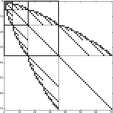
(a) $N=4$, $P=4$ gives $350$ blocks

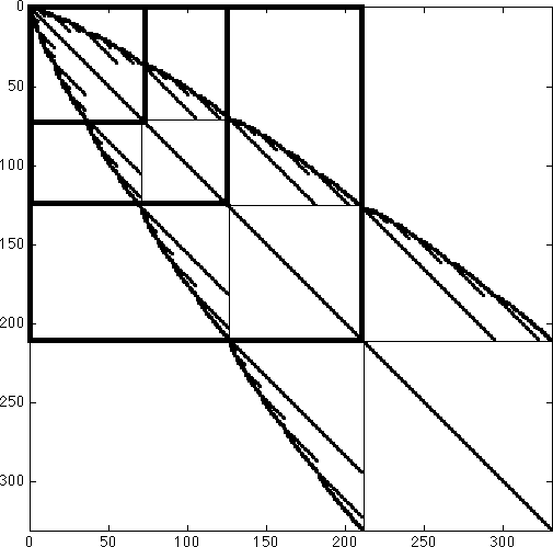
(b) $N=4$, $P=7$ gives $2010$ blocks

Figure 1: Hierarchical structure of the matrix $c_{P}$ which determines the block sparsity of the global stochastic Galerkin matrix with $N=4$ stochastic dimensions using 1(a) $P=4$, or 1(b) $P=7$ order of polynomial expansion. The sub-blocks correspond to the polynomials of order 1(a) $P=1,2,3$ and 1(b) $P=4,5,6$.

3 Structure of the model matrices

Let us begin by an illustration. Figure 1(a) shows the structure of the stochastic Galerkin matrix based on the fourth order polynomial chaos expansion in four stochastic dimensions. The schematic matrix in the picture is$~{}c_{P}$ (here $P=4$), so in the global stochastic Galerkin matrix as it is written in eq. (12) each tile corresponds to a block of a stiffness matrix with the same sparsity pattern as the original finite element problem. Now, let us denote the corresponding global Galerkin matrix by$~{}A_{4}$ , and by $A_{3}$, $B_{4}$, $C_{4}$ and $D_{4}$ its four submatrices, cf. (15). We see that$~{}D_{4}$ is block diagonal and the structure of$~{}A_{3}$ resembles the structure of$~{}A_{4}$ and this hierarchy is repeated all the way to the $1\times 1$ block$~{}A_{0}$ and a block diagonal matrix$~{}D_{1}$. The number in the subscript indicates that the entries in the block correspond to the polynomial expansion in the case of (a) $A_{3}$ of order three or less, and (b) $B_{3},\ C_{3}\$and$\ D_{3}$ of order three. Clearly, the sparsity and hierarchical structure follows from orthogonality of the polynomials as was pointed out in [25]. More specifically, let us consider a two-by-two block structure of a (square) coefficient matrix $c_{P}$ with dimensions $\frac{\left(N+P\right)!}{N!P!}$ as

$$c_{P}=\left[\begin{array}[c]{cc}c_{P-1}&b_{P}^{T}\\ b_{P}&d_{P}\end{array}\right],$$

where $c_{P-1}$ is the first principal submatrix with dimensions $\frac{\left(N+P-1\right)!}{N!\left(P-1\right)!}$, and the remaining blocks are defined accordingly. Generally, let us consider a recursive hierarchy in the spliting of $c_{P}$ as

$$c_{\ell}=\left[\begin{array}[c]{cc}c_{\ell-1}&b_{\ell}^{T}\\ b_{\ell}&d_{\ell}\end{array}\right],\qquad\ell=P,\dots,1,$$

where the dimensions of$~{}c_{\ell}$ are given by $\frac{\left(N+\ell\right)!}{N!\ell!}$, the dimensions of the first principal submatrices$~{}c_{\ell-1}$ are given by $\frac{\left(N+\ell-1\right)!}{N!\left(\ell-1\right)!}$, and the remaining blocks are defined accordingly. We note that even though the matrices$~{}c_{\ell}$ are symmetric, the stochastic Galerkin matrix will be symmetric only if each one of the matrices$~{}K_{i}$ is itself symmetric. We refer, e.g., to [9, 30] for further details and discussion, and state here only the essential observation for our approach:

Lemma 3 ([9, Corollary 2.6]).

The block $d_{\ell}$ is a diagonal matrix for all $\ell=1,\dots,P$.

The global problem (12) can be equivalently written as

$$A_{P}u_{P}=f_{P},$$ (14)

with the matrix $A_{P}$ having a hierarchical structure

$$A_{\ell}=\left[\begin{array}[c]{cc}A_{\ell-1}&B_{\ell}\\ C_{\ell}&D_{\ell}\end{array}\right],\qquad\ell=P,\dots,1,$$ (15)

where the subscript$~{}\ell$ stands for the blocks obtained by an approximation by the $\ell-$th degree stochastic polynomial (or lower), and all of the blocks $D_{\ell}$ are block diagonal. In particular the smallest case is given by the finite element approximation with the mean values of the coefficients, and therefore the mean-value problem is

$$A_{0}u_{0}=f_{0},$$ (16)

and in particular $A_{0}=K_{0}$. In this paper, we will assume that the inverse of $A_{0}$ is known, or at least that we have a good preconditioner $M_{0}$ readily available.

Remark 4.

Clearly, if all of the matrices$~{}K_{i}$ are symmetric, the global matrix$~{}A_{P}$ and all of its submatrices$~{}A_{\ell}$ will be symmetric as well, i.e.,

$$A_{\ell}=\left[\begin{array}[c]{cc}A_{\ell-1}&B_{\ell}\\ B_{\ell}^{T}&D_{\ell}\end{array}\right],\qquad\ell=P,\dots,1.$$

However, for the sake of generality, we will use the non-symmetric notation (15). We note that a question under what conditions is the global problem positive definite is far more delicate, in general depends on the type of the polynomial expansion and also on the choice of the covariance function.

In the next section we introduce our preconditioner, taking advantage of the hierarchical structure and of the fact that the matrices $D_{\ell}$, where $\ell=P,\dots,1$, are block diagonal.

4 Schur complement preconditioner

Let us find an inverse of a general block matrix given as

$$\left[\begin{array}[c]{cc}A&B\\ C&D\end{array}\right],$$ (17)

assuming that we can easily compute the inverse of $D$. By block LU decomposition, we can derive

$$\left[\begin{array}[c]{cc}A&B\\ C&D\end{array}\right]=\left[\begin{array}[c]{cc}I_{A}&BD^{-1}\\ 0&I_{D}\end{array}\right]\left[\begin{array}[c]{cc}S&0\\ 0&D\end{array}\right]\left[\begin{array}[c]{cc}I_{A}&0\\ D^{-1}C&I_{D}\end{array}\right],$$ (18)

where $S=A-BD^{-1}C$ is the Schur complement of$~{}D$ in (17). Inverting the three blocks, we obtain

$$\left[\begin{array}[c]{cc}A&B\\ C&D\end{array}\right]^{-1}=\left[\begin{array}[c]{cc}I_{A}&0\\ -D^{-1}C&I_{D}\end{array}\right]\left[\begin{array}[c]{cc}S^{-1}&0\\ 0&D^{-1}\end{array}\right]\left[\begin{array}[c]{cc}I_{A}&-BD^{-1}\\ 0&I_{D}\end{array}\right].$$ (19)

The hierarchical Schur complement preconditioner is based on the block inverse (19). In the action of the preconditioner, application of the three blocks on the right-hand side of (19) will be called (in the order in which they are performed) as pre-correction, correction and post-correction.

So, in the action of the preconditioner we would like to approximate problem (14) which with respect to (15) can be written as

$$\left[\begin{array}[c]{cc}A_{P-1}&B_{P}\\ C_{P}&D_{P}\end{array}\right]\left[\begin{array}[c]{c}u_{P}^{P-1}\\ u_{P}^{P}\end{array}\right]=\left[\begin{array}[c]{c}f_{P}^{P-1}\\ f_{P}^{P}\end{array}\right].$$ (20)

The matrix inverse can be with respect to (19) written as

$$\left[\begin{array}[c]{cc}A_{P-1}&B_{P}\\ C_{P}&D_{P}\end{array}\right]^{-1}=\left[\begin{array}[c]{cc}I_{A}&0\\ -D_{P}^{-1}C_{P}&I_{D}\end{array}\right]\left[\begin{array}[c]{cc}S_{P-1}^{-1}&0\\ 0&D_{P}^{-1}\end{array}\right]\left[\begin{array}[c]{cc}I_{A}&-B_{P}D_{P}^{-1}\\ 0&I_{D}\end{array}\right],$$

where

$$S_{P-1}=A_{P-1}-B_{P}D_{P}^{-1}C_{P}.$$

Because computing (and inverting) the Schur complement $S_{P-1}$ explicitly is computationally prohibitive, we suggest to replace the inverse of $S_{P-1}$ by the inverse of $A_{P-1}$. Since $A_{P-1}$ has the hierarchical structure as described by (15), i.e.,

$$A_{P-1}=\left[\begin{array}[c]{cc}A_{P-2}&B_{P-1}\\ C_{P-1}&D_{P-1}\end{array}\right],$$

we can approximate its inverse again using the idea of (19) and so on. Eventually, we arrive at the Schur complement of the mean-value problem$~{}S_{0}$ which we replace by$~{}A_{0}$. Thus the action of this hierarchical preconditioner$~{}M_{P}$ consists of a number of pre-correction steps performed on the levels$~{}\ell=P,\dots,1$, solving the “mean-value” problem with$~{}A_{0}$ on the lowest level, and performing a number of the post-processing steps sweeping up the levels. We now formulate the preconditioner for the iterative solution of the global problem (14) more concisely as:

Algorithm 5 (Hierarchical Schur complement preconditioner).

The preconditioner $M_{P}:r_{P}\longmapsto u_{P}$ is defined as follows:

for $\ell=P,\ldots 1$,

split the residual, based on the hierarchical structure of matrices, as

$$r_{\ell}=\left[\begin{array}[c]{c}r_{\ell}^{\ell-1}\\ r_{\ell}^{\ell}\end{array}\right],$$

compute the pre-correction as

$$g_{\ell-1}=r_{\ell}^{\ell-1}-B_{\ell}D_{\ell}^{-1}r_{\ell}^{\ell}.$$

If $\ell>1$, set

$$r_{\ell-1}=g_{\ell-1}.$$

Else (if $\ell=1)$, solve the system $A_{0}u_{0}=g_{0}$.

end

for $\ell=1,\ldots P$,

compute the post-correction, i.e., set $u_{\ell}^{\ell-1}=u_{\ell-1}$, solve

$$u_{\ell}^{\ell}=D_{\ell}^{-1}\left(r_{\ell}^{\ell}-C_{\ell}u_{\ell}^{\ell-1}\right),$$

and concatenate

$$u_{\ell}=\left[\begin{array}[c]{c}u_{\ell}^{\ell-1}\\ u_{\ell}^{\ell}\end{array}\right].$$

If $\ell<P,$ set $u_{\ell+1}^{\ell}=u_{\ell}$.

end

We will now restrict our considerations to the case when all of the matrices  $A_{\ell}$, $\ell=P,\dots,1$ are symmetric, positive definite. In this case, the decomposition (18) can be written for all levels $\ell$ as

$$A_{\ell}=\left[\begin{array}[c]{cc}A_{\ell-1}&B_{\ell}\\ B_{\ell}^{T}&D_{\ell}\end{array}\right]=\left[\begin{array}[c]{cc}I_{A}&B_{\ell}D_{\ell}^{-1}\\ 0&I_{D}\end{array}\right]\left[\begin{array}[c]{cc}S_{\ell-1}&0\\ 0&D_{\ell}\end{array}\right]\left[\begin{array}[c]{cc}I_{A}&0\\ D_{\ell}^{-1}B_{\ell}^{T}&I_{D}\end{array}\right].$$

Because all of the matrices $A_{\ell}$, $\ell=P,\dots,1$ are positive definite, the above becomes a set of congruence transformations and by the Sylvester law of inertia, all of the Schur complements$~{}S_{\ell}$, $\ell=P-1,\dots,0$ are also symmetric positive definite. Thus, we can establish for appropriate vectors $u$ the next set of inequalities,

$$c_{\ell,1}\left\|u\right\|_{A_{\ell}}^{2}\leq\left\|u\right\|_{S_{\ell}}^{2}\leq c_{\ell,2}\left\|u\right\|_{A_{\ell}}^{2},\qquad\ell=0,\dots,P-1,$$ (21)

where $\left\|u\right\|_{A}^{2}=u^{T}Au$ denotes the energy norm, and use it in the following:

Theorem 6.

For the symmetric, positive definite matrix$~{}A_{P}$ the preconditioner$~{}M_{P}$ defined by Algorithm 5 is also positive definite, and the condition number $\kappa$ of the preconditioned system is bounded by

$$\kappa=\frac{\lambda_{\max}\left(M_{P}A_{P}\right)}{\lambda_{\min}\left(M_{P}A_{P}\right)}\leq C,\qquad\text{where }C=\Pi_{\ell=0}^{P-1}\frac{c_{\ell,2}}{c_{\ell,1}}.$$

Proof.

The bound follows directly from the sequential replacement of the Schur complement operators $S_{\ell}$ by the hierarchical matrices $A_{\ell}$ in Algorithm 5, and the bounds in the equivalence (21). ∎

Hence, the convergence rate can be established from the spectral equivalence (21).

Remark 7.

Despite the multiplicative growth of the condition number bound as predicted by Theorem 6 from our numerical experiments (Table 2) it appears that, at least in the case of uniform random variables and Legendre polynomials, the ratio of the constants in (21) is close to one and hence the convergence of conjugate gradients is not as pessimistic as predicted by the bound.

In the next section, we discuss several modifications of the method and the preconditioner.

5 Variants and implementation remarks

Clearly, there are many other ways of setting up a hierarchical preconditioner. These possibilities follow by considering the block inverse (19) and writing it in a more general form, which can be subsequently used in the approximation of the preconditioner from Algorithm 5, as

$$M=\left[\begin{array}[c]{cc}I_{A}&0\\ -M_{D}^{3}C&I_{D}\end{array}\right]\left[\begin{array}[c]{cc}M_{S}&0\\ 0&M_{D}^{2}\end{array}\right]\left[\begin{array}[c]{cc}I_{A}&-BM_{D}^{1}\\ 0&I_{D}\end{array}\right],$$ (22)

so that $M_{D}^{i}$ , $i=1,2,3$, approximate $D^{-1}$ and$~{}M_{S}$ approximates$~{}S^{-1}$. Our main approximation in Algorithm 5 is in using the hierarchy of matrices $A_{\ell}$, $\ell=P-1,\dots,0$ in place of$~{}M_{S}$ on each level. Next, in our case$~{}D$ is block-diagonal. Thus computing its inverse means solving independently a number of systems, where each one of them has the same size (and sparsity structure) as the deterministic problem for the mean. In fact, the diagonal blocks are just scalar multiples of the “mean-value” matrix$~{}K_{0}(=A_{0})$. In our implementation, we have replaced the exact solves of$~{}D$ by independent loops of preconditioned Krylov subspace iterations for each diagonal block of$~{}D$ using the mean-value preconditioner$~{}M_{0}$. In the numerical experiments we have tested convergence with the following choices of$~{}M_{0}$: no preconditioner, simple diagonal preconditioner, and the exact LU decomposition of the block$~{}A_{0}$ (which converges in one iteration). So this variant of the hierarchical Schur complement preconditioner involves multiple loops of inner iterations and thus possibly changes in every outer iteration. In order to accommodate such variable preconditioner, it is generally recommended to use a flexible Krylov subspace method such as flexible CG [26], FGMRES [27], or GMRESR [28]. Nevertheless, we have observed essentially the same convergence in terms of outer iterations with both variants of the conjugate gradients, the flexible and the standard one as well. The convergence seems also to be independent of the choice of$~{}M_{0}$ and in this contribution we do not advocate any specific choice. Next, one can in general replace the action of any$~{}M_{D}^{i}$, $i=1,2,3$, by the action of just$~{}M_{0}$ itself. However it is well-known from iterative substructuring cf., e.g., [11, Section 4.4], that even if $M_{D}$ is spectrally equivalent to$~{}D^{-1}$, the resulting preconditioner might not be spectrally equivalent to the original problem.

It also appears that one can modify not only the preconditioner, but also the set up of the method itself. Namely, inspired by the iterative substructuring cf., e.g., [12], one can reduce the system given by$~{}A_{P}$ to the system given by the Schur complement $S_{P-1}$ used subsequently in the iterations. So, in the first step, cf. (20), we eliminate $u_{P}^{P}$ and define $u_{P-1}\equiv u_{P}^{P-1}$, which yields

$$S_{P-1}u_{P-1}=g_{P-1},$$ (23)

where

$$S_{P-1}=A_{P-1}-B_{P}D_{P}^{-1}C_{P},\quad\text{and}\quad g_{P-1}=f_{P}^{P-1}-B_{P}D_{P}^{-1}f_{P}^{P}.$$

After convergence, the variables $u_{P}^{P}$ are recovered from

$$u_{P}^{P}=D_{P}^{-1}\left(f_{P}^{P}-C_{P}u_{P-1}\right).$$

There are two advantages of the a-priori elimination of the second block: first, because the system (23) will be solved iteratively, the iterations can be performed on a much smaller system and also, at least for symmetric, positive definite problems, the condition number of the Schur complement cannot be higher than the one of the original problem [11] even if one uses a diagonal preconditioning [31]. The preconditioner $M_{P-1}$ for the system (23) is then the same as in Algorithm 5 except that the for-loops are performed only for all levels$~{}\ell=1,\dots,P-1$. However, this reduction is theoretically justified only when exact solves for the block diagonal matrix $D_{P}$ are available. In general, if one uses only approximate solves, e.g., by performing inner/outer Krylov iterations for $D_{P}$ and $S_{P-1}$ respectively, the global system matrix becomes variable as well, this might lead to the loss of orthogonality and poor performance of the method. Our numerical experiments indicated that the preconditioned iterations for $A_{P}$ and $S_{P-1}$ perform identically, but we do not advocate to use a-priori reduction to the Schur complement in general.

6 Numerical examples

We have implemented the stochastic Galerkin finite element method for the model elliptic problem (1)-(2) on a square domain $\left[0,1\right]\times\left[0,1\right]$ uniformly discretized by $10\times 10$ Lagrangean bilinear finite elements. The mean value of the coefficient$~{}k$ was set to $k_{0}=1$. The coefficients in the covariance function $C$ defined by eq. (8) were set to $L=0.5$ and $\sigma=0.5$, so the coefficient of variation is given as $CoV=\sigma/k_{0}=\sigma=50\%$. The $15$ dominant eigenvalues of the discretized eigenvalue problem (7) are shown in Figure 2. We have studied convergence of the flexible version of the conjugate gradient method (FCG) without a preconditioner, with a global mean-based preconditioner$~{}M_{\mathrm{m}}$ by Powell and Elman [6], with the block symmetric Gauss-Seidel preconditioner $M_{\mathrm{bGS}}$ (with zero initial guess) and with the hierarchical Schur complement preconditioner$~{}M_{\mathrm{HS}}$. The convergence results are summarized in Tables 1-4. We have observed essentially the same convergence of the standard conjugate gradients compared to the flexible version, which is reported in the tables. Also, in our experience, the convergence rates were independent of the choice of the mean-value preconditioner$~{}M_{0}$ (no preconditioner, diagonal preconditioner and the LU-decomposition of the “mean-value” block$~{}A_{0}$) used in inner iterations of the preconditioner for the diagonal block solves with the same relative residual tolerance as in the outer iterations. From Tables 1 and 2 it appears that the convergence depends only mildly on the stochastic dimension$~{}N$ and the order of polynomial expansion$~{}P$, respectively. Table 3 indicates a modest dependence on the value of the standard deviation $\sigma$, and finally Table 4 indicates that the convergence is independent of the mesh size$~{}h$. We note that for $CoV>55\%$ the problem is no longer guaranteed to be elliptic, and the global matrix$~{}A$ is not positive definite.

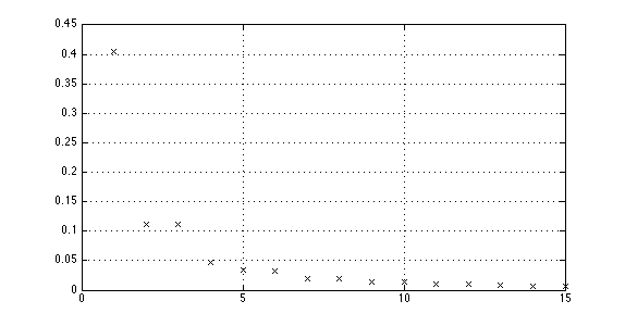
Figure 2: The $15$ dominant eigenvalues with the covariance kernel (8) (in this plot $\sigma=1)$.

Table 1: Convergence of (flexible) conjugate gradients for the full system matrix $A$, for $A$ preconditioned by the mean-based preconditioner $M_{\mathrm{m}}$, by the block Gauss-Seidel preconditioner $M_{\mathrm{bGS}}$, and by the hierarchical Schur complement preconditioner $M_{\mathrm{HS}}$. The coefficient of variation of the uniform random field is $CoV=50\%$, polynomial degree is $P=4$, and the stochastic dimension $N$ is variable. Here, $ndof$ is the dimension of $A$, $iter$ is the number of iterations with the relative residual tolerance $10^{-8}$, and $\kappa$ is the condition number estimate from the Lánczos sequence in conjugate gradients.

setup		$A$		$M_{\mathrm{m}}A$		$M_{\mathrm{bGS}}A$		$M_{\mathrm{HS}}A$
$N$	$ndof$	$iter$	$\kappa$	$iter$	$\kappa$	$iter$	$\kappa$	$iter$	$\kappa$
1	605	173	1965.4	12	2.0127	5	1.0507	5	1.0465
2	1815	531	5333.3	15	2.7340	6	1.1279	6	1.1236
3	4235	745	9876.9	16	2.9995	7	1.1693	6	1.1514
4	8470	902	17,150.2	17	3.3413	7	1.2131	7	1.2028
5	15,246	1033	17,275.8	18	3.5891	7	1.2447	7	1.2434
6	25,410	1037	17,333.5	18	3.6349	7	1.2501	7	1.2559
7	39,930	1040	17,348.9	19	4.0993	8	1.3202	7	1.3146
8	59,895	1081	17,360.6	19	4.0597	8	1.3198	7	1.3182

Table 2: Convergence of (flexible) conjugate gradients for the full system matrix $A$, for $A$ preconditioned by the mean-based preconditioner $M_{\mathrm{m}}$, by the block Gauss-Seidel preconditioner $M_{\mathrm{bGS}}$, and by the hierarchical Schur complement preconditioner $M_{\mathrm{HS}}$. The stochastic dimension is $N=4$, $CoV=50\%$, and the polynomial degree $P$ is variable. The other headings are same as in Table 1.

setup		$A$		$M_{\mathrm{m}}A$		$M_{\mathrm{bGS}}A$		$M_{\mathrm{{HS}}}A$
$P$	$ndof$	$iter$	$\kappa$	$iter$	$\kappa$	$iter$	$\kappa$	$iter$	$\kappa$
1	605	134	625.6	9	1.6391	5	1.0626	5	1.0624
2	1815	315	1903.2	13	2.2379	6	1.1117	6	1.1109
3	4235	586	5721.1	15	2.8122	7	1.1658	6	1.1559
4	8470	902	17,150.2	17	3.3413	7	1.2131	7	1.2028
5	15,246	1402	29,751.0	18	3.7824	7	1.2538	7	1.2426
6	25,410	1943	49,842.4	19	4.1534	8	1.2921	7	1.2798
7	39,930	2568	83,056.6	20	4.4708	8	1.3219	7	1.3125
8	59,895	3267	136,419.0	20	4.7371	8	1.3472	7	1.3398

Table 3: Convergence of (flexible) conjugate gradients for the full system matrix $A$, its first Schur complement $S$, for $A$ preconditioned by the global mean-based preconditioner $M_{\mathrm{m}}$, by the block Gauss-Seidel preconditioner $M_{\mathrm{bGS}}$, and by the hierarchical Schur complement preconditioner $M_{\mathrm{HS}}$. Here, the size of $A$ is $8470$ $ndof$, the stochastic dimension is $N=4$, the polynomial degree is $P=4$, the mean is $k_{0}=1$, and the coefficient of variation $CoV$ is variable. The other headings are same as in Table 1.

setup	$A$		$M_{\mathrm{m}}A$		$M_{\mathrm{bGS}}A$		$M_{\mathrm{{HS}}}A$
$CoV(\%)$	$iter$	$\kappa$	$iter$	$\kappa$	$iter$	$\kappa$	$iter$	$\kappa$
5	694	15,556.3	6	1.0960	3	1.0008	3	1.0009
15	739	15,673.2	9	1.3514	4	1.0090	4	1.0089
25	804	15,912.5	11	1.7021	5	1.0314	5	1.0304
35	833	16,286.1	13	2.1808	6	1.0770	5	1.0664
45	877	16,815.9	16	2.8773	6	1.1510	6	1.1414
55	926	17,539.6	19	3.9523	8	1.2948	7	1.2830

Table 4: Convergence of (flexible) conjugate gradients for the full system matrix $A$, for $A$ preconditioned by the global mean-based preconditioner $M_{\mathrm{m}}$, by the block Gauss-Seidel preconditioner $M_{\mathrm{bGS}}$, and by the hierarchical Schur complement preconditioner $M_{\mathrm{HS}}$. Here, the stochastic dimension is $N=4$, the polynomial degree is $P=4$, the mean is $k_{0}=1$, the coefficient of variation is $CoV=50\%$, and the size of the finite element mesh $h$ is variable. The other headings are same as in Table 1.

setup		$A$		$M_{\mathrm{m}}A$		$M_{\mathrm{bGS}}A$		$M_{\mathrm{{HS}}}A$
$h$	$ndof$	$iter$	$\kappa$	$iter$	$\kappa$	$iter$	$\kappa$	$iter$	$\kappa$
$1/5$	2520	404	4847.5	16	3.2484	7	1.2022	6	1.1790
$1/10$	8470	902	17,150.2	17	3.3413	7	1.2131	7	1.2028
$1/15$	17,920	1386	36,716.6	17	3.3145	7	1.2063	7	1.2047
$1/20$	30,870	1883	63,535.2	17	3.3463	7	1.2110	7	1.2032
$1/25$	47,320	2383	97,605.6	17	3.3473	7	1.2112	7	1.2032
$1/30$	67,270	2872	138,929.0	17	3.3190	7	1.2070	7	1.2054

Table 5: Numbers of blocks in the full system matrix and the “work-count” in the application of the preconditioner $M$, when one of the parameters $N$ or $P$ is changing and the other one is set to $4$, cf. Figure 1. Here $n_{b}$ is the total number of blocks, $n_{db}$ is the number of diagonal blocks, which is the same as the number of solves in the application of the mean-based preconditioner $M_{m}$, $n_{m}$ is the number of block matrix-vector multiplications in the action of the preconditioner $M$, and $n_{ds}$ is the number of its block diagonal solves.

$N$ or $P$	$n_{b}$	$n_{db}$	$n_{m}$	$n_{ds}$
1	13	5	8	9
2	55	15	40	29
3	155	35	120	69
4	350	70	280	139
5	686	126	560	251
6	1218	210	1008	419
7	2010	330	1680	659
8	3135	495	2640	989

Table 5 summarizes the block count in the structure of the global Galerkin matrix$~{}A$ obtained using the KL expansion, cf. Figure 1, when either of the parameters $N$ or $P$ changes and the other one is set to be equal to four. The two choices lead to slightly different block sparsity structures of $A$, however the numbers of blocks are the same. Let us denote by $n_{b}$ the total number of blocks in$~{}A$ and by $n_{db}$ the number of its diagonal blocks. Note that one application of the mean-based preconditioner requires $n_{db}$ solves of the diagonal blocks. The columns three and four in Table 5 contain the numbers of block matrix-vector multiplications$~{}n_{m}$ and block diagonal solves$~{}n_{ds}$ performed in one action of the hierarchical Schur preconditioner. From Algorithm 5 we obtain that

$$n_{m}=n_{b}-n_{db},$$

where half of multiplications is performed in the first for-loop and the other half in the second, and

$$n_{ds}=2(n_{db}-1)+1,$$

which follows from the two for-loops and one solve of the first block$~{}A_{0}$. Hence one action of the hierarchical Schur preconditioner requires nearly the same number of computations as one global Galerkin matrix-vector multiplications, $n_{m}\approx n_{b}$, and two applications of the mean-based preconditioner, $n_{ds}\approx 2n_{db}$. It is important to note that whereas the application of the mean-based preconditioner can be performed fully in parallel, the two for-loops in Algorithm 5 are sequential, and thus the eventual parallelization can be performed only within each step of these for-loops. The work count of  $M_{\mathrm{bGS}}$, which is block sequential, is given by $2n_{db}$ diagonal solves, and $1.5$ (or $2$, if the initial guess of GS is nonzero) times of block matrix-vector multiplications compared to $M_{\mathrm{HS}}$.

In the second set of experiments, we have tested convergence of the preconditioner with the same physical domain and parameter setting, except assuming that the random coefficient$~{}k$ has lognormal distribution with the coefficient of variation being set to $CoV=\sigma_{\log}/\mu_{\log}=100\%$. We note that in order to guarantee existence and uniqueness of the solution, we have used twice the order of polynomial expansion of the coefficient$~{}k$ than of the solution, cf. [32]. Such discretization is done within the gPC framework, see Remark 1, using Hermite polynomials [33], and leads to a fully block dense structure of the global Galerkin matrix$~{}A$. Therefore the solves involving submatrices$~{}D_{\ell}$, $\ell=1,\dots,P$, in the pre- and post-correction steps are no longer block diagonal. Our numerical tests using both, direct and iterative solves with the$~{}D_{\ell}$, and using the same tolerance as for the outer iterations, lead to the same count of outer iterations. The performance results are summarized in Tables 6-9. The convergence rate reported in Table 6 indicates a mild dependence on the stochastic dimension$~{}N$, Table 7 indicates a modest dependence on the order of the polynomial expansion$~{}P$, and Table 8 indicates also a modest dependence on the coefficient of variation$~{}CoV$. From Table 9 we see that the convergence is nearly independent of the mesh size$~{}h$. The performance of both preconditioners $M_{\mathrm{bGS}}$ and $M_{\mathrm{HS}}$ is significantlly better compared to the mean-based preconditioner $M_{\mathrm{m}}$. Also, we see that $M_{\mathrm{HS}}$ performs a bit better than $M_{\mathrm{bGS}}$. However, we must note that  $M_{\mathrm{HS}}$ is also more computationally intensive because it requires solves with larger diagonal submatrices$~{}D_{\ell}$, for all levels $\ell=1,\dots,P$, and a work count comparison with $M_{\mathrm{bGS}}$ is not straightforward. As before, the two for-loops corresponding to Algorithm 5 are sequential, and thus the eventual paralelisation can be performed only within each step in the for-loop.

Table 6: Convergence of (flexible) conjugate gradients for the full system matrix $A$ obtained by the gPC expansion of the lognormal field, for $A$ preconditioned by the mean-based preconditioner $M_{\mathrm{m}}$, by the block Gauss-Seidel preconditioner $M_{\mathrm{bGS}}$, and by the hierarchical Schur complement preconditioner $M_{\mathrm{HS}}$. Polynomial degree is fixed to $P=4$, the coefficient of variation of the lognormal random field is $CoV=100\%$, and the stochastic dimension $N$ is variable. The other headings are same as in Table 1.

setup		$A$		$M_{\mathrm{m}}A$		$M_{\mathrm{bGS}}A$		$M_{\mathrm{{HS}}}A$
$N$	$ndof$	$iter$	$\kappa$	$iter$	$\kappa$	$iter$	$\kappa$	$iter$	$\kappa$
1	605	585	51,376.4	48	28.7589	15	3.4192	15	3.4000
2	1815	1396	58,718.8	61	37.1593	17	3.7490	16	3.6244
3	4235	1770	69,054.8	62	38.0715	17	3.7380	16	3.7632
4	8470	2016	70,143.6	66	43.6525	19	4.2935	16	4.1669

Table 7: Convergence of (flexible) conjugate gradients for the full system matrix $A$ obtained by the gPC expansion of the lognormal field, for $A$ preconditioned by the mean-based preconditioner $M_{\mathrm{m}}$, by the block Gauss-Seidel preconditioner $M_{\mathrm{bGS}}$, and by the hierarchical Schur complement preconditioner $M_{\mathrm{HS}}$. Stochastic dimension is fixed to $N=4$, the coefficient of variation of the lognormal random field is $CoV=100\%$, and the polynomial degree $P$ is variable. The other headings are same as in Table 1.

setup		$A$		$M_{\mathrm{m}}A$		$M_{\mathrm{bGS}}A$		$M_{\mathrm{{HS}}}A$
$P$	$ndof$	$iter$	$\kappa$	$iter$	$\kappa$	$iter$	$\kappa$	$iter$	$\kappa$
1	605	134	578.2	15	3.4954	8	1.3910	7	1.3856
2	1815	329	2027.3	28	8.9450	12	1.9742	10	1.9289
3	4235	804	10,048.4	44	20.0366	15	2.8670	13	2.7955
4	8470	2016	70,143.6	66	43.6525	19	4.2935	16	4.1669

Table 8: Convergence of (flexible) conjugate gradients for the full system matrix $A$ obtained by the gPC expansion of the lognormal field, for $A$ preconditioned by the mean-based preconditioner $M_{\mathrm{m}}$, by the block Gauss-Seidel preconditioner $M_{\mathrm{bGS}}$, and by the hierarchical Schur complement preconditioner $M_{\mathrm{HS}}$. Here, the size of $A$ is $8470$ $ndof$, the stochastic dimension is $N=4$, the polynomial degree is $P=4$, and the coefficient of variation of the lognormal field $CoV$ is variable. The other headings are same as in Table 1.

setup	$A$		$M_{\mathrm{m}}A$		$M_{\mathrm{bGS}}A$		$M_{\mathrm{{HS}}}A$
$CoV\,(\%)$	$iter$	$\kappa$	$iter$	$\kappa$	$iter$	$\kappa$	$iter$	$\kappa$
25	719	7378.4	16	3.2356	7	1.1761	7	1.1776
50	1039	16,014.8	29	9.3553	11	1.7685	10	1.7836
75	1511	35,317.3	46	22.2147	15	2.8198	13	2.8454
100	2016	70,143.6	66	43.6525	19	4.2935	16	4.1669
125	2591	116,678.0	85	72.7584	23	5.9776	19	5.5362
150	3209	178,890.0	103	107.0670	26	7.7459	21	6.8507

Table 9: Convergence of (flexible) conjugate gradients for the full system matrix $A$ obtained by the gPC expansion of the lognormal field, for $A$ preconditioned by the mean-based preconditioner $M_{\mathrm{m}}$, by the block Gauss-Seidel preconditioner $M_{\mathrm{bGS}}$, and by the hierarchical Schur complement preconditioner $M_{\mathrm{HS}}$. Here, the stochastic dimension is $N=4$, the polynomial degree is $P=4$, the coefficient of variation of the lognormal random field is $CoV=100\%$, and the size of the finite element mesh $h$ is variable. The other headings are same as in Table 1.

setup		$A$		$M_{\mathrm{m}}A$		$M_{\mathrm{bGS}}A$		$M_{\mathrm{{HS}}}A$
$h$	$ndof$	$iter$	$\kappa$	$iter$	$\kappa$	$iter$	$\kappa$	$iter$	$\kappa$
$1/5$	2520	831	17,695.3	59	40.6232	18	3.9885	15	3.8361
$1/10$	8470	2016	70,143.6	66	43.6525	19	4.2935	16	4.1669
$1/15$	17,920	3377	158,334.0	68	44.4170	19	4.3764	16	4.2394
$1/20$	30,870	4395	275,686.0	69	44.8882	19	4.3742	17	4.2510
$1/25$	47,320	5600	429,551.0	69	44.9413	20	4.3986	17	4.2592
$1/30$	67,270	7180	626,475.0	71	45.1100	19	4.3732	17	4.2630

The numerical experiments presented here were implemented using a sequential code in Matlab, version 7.12.0.635 (R2011a), and therefore we do not report on computational times.

7 Conclusion

We have presented a hierarchical Schur complement preconditioner for the iterative solution of the systems of linear algebraic equations obtained from the stochastic Galerkin finite element discretizations. The preconditioner takes an advantage of the recursive hierarchical two-by-two structure of the global matrix, with one of the submatrices block diagonal. We have compared its convergence using (flexible) conjugate gradients without any preconditioner, with the mean-based preconditioner which requires one block diagonal solve per iteration, and with the block version of the well-known symmetric Gauss-Seidel method used as a preconditioner. The algorithm of our preconditioner consists of a loop of diagonal block solves and a multiplication by the upper block triangle in the pre-correction loop, and of another loop of diagonal block solves and a multiplication by the lower block triangle in the post-correction loop. The loops are sequential throughout the hierarchy of the global matrix, but the block solves are independent within each level. We have also succesfully tested the preconditioner in the case of the random coefficient with lognormal distribution. However, in this case the algorithm involves solves (either direct or of preconditioned inner iterations) with larger submatrices than just the diagonal blocks, and a direct comparison to the symmetric block Gauss-Seidel preconditioner in terms of work count is not straightforward.

In conclusion, our algorithm appears to be more effective in terms of iterations and work count compared to the block version of the symmetric Gauss-Seidel method. Our method also allows for the same degree of parallelism as the Gauss-Seidel method, since both involve solving the block diagonal matrices $D_{\ell}$. It is important to note that the discussed preconditioners in general rely only on (block-by-block) matrix-vector multiplies, and their performance will also depend on the choice of preconditioner$~{}M_{0}$ for the solves with the diagonal blocks. Clearly, one can use such solver for each one of the diagonal blocks that might introduce another level of parallelism, e.g., similarly as recently proposed in [34, 35, 36]. However such extensions will be studied elsewhere.

References

- [1] Babuška I, Nobile F, Tempone R. A stochastic collocation method for elliptic partial differential equations with random input data. SIAM Review 2010; 52(2):317–355, 10.1137/100786356. (The paper originally appeared in SIAM Journal on Numerical Analysis, Volume 45, Number 3, 2007, pages 1005–1034.).
- [2] Xiu D, Hesthaven JS. High-order collocation methods for differential equations with random inputs. SIAM Journal on Scientific Computing 2005; 27(3):1118–1139, 10.1137/040615201.
- [3] Babuška I, Tempone R, Zouraris GE. Galerkin finite element approximations of stochastic elliptic partial differential equations. SIAM Journal on Numerical Analysis 2005; 42(2):800–825, 10.1137/S0036142902418680.
- [4] Babuška I, Tempone R, Zouraris G. Solving elliptic boundary value problems with uncertain coefficients by the finite element method: the stochastic formulation. Computer Methods in Applied Mechanics and Engineering 2005; 194(12-16):1251–1294, 10.1016/j.cma.2004.02.026.
- [5] Ghanem RG, Spanos PD. Stochastic Finite Elements: A Spectral Approach. Springer-Verlag New York, Inc.: New York, NY, USA, 1991. (Revised edition by Dover Publications, 2003).
- [6] Powell CE, Elman HC. Block-diagonal preconditioning for spectral stochastic finite-element systems. IMA Journal of Numerical Analysis 2009; 29(2):350–375, 10.1093/imanum/drn014.
- [7] Ernst OG, Powell CE, Silvester DJ, Ullmann E. Efficient solvers for a linear stochastic Galerkin mixed formulation of diffusion problems with random data. SIAM Journal on Scientific Computing 2009; 31(2):1424–1447, 10.1137/070705817.
- [8] Ullmann E, Elman H, Ernst O. Efficient iterative solvers for stochastic galerkin discretizations of log-transformed random diffusion problems. SIAM Journal on Scientific Computing 2012; 34(2):A659–A682, 10.1137/110836675.
- [9] Rosseel E, Vandewalle S. Iterative solvers for the stochastic finite element method. SIAM Journal on Scientific Computing 2010; 32(1):372–397, 10.1137/080727026.
- [10] Keese A, Matthies HG. Hierarchical parallelisation for the solution of stochastic finite element equations. Computers and Structures 2005; 83(14):1033–1047, 10.1016/j.compstruc.2004.11.014.
- [11] Smith BF, Bjørstad PE, Gropp WD. Domain decomposition: parallel multilevel methods for elliptic partial differential equations. Cambridge University Press: Cambridge, 1996.
- [12] Toselli A, Widlund OB. Domain Decomposition Methods—Algorithms and Theory, Springer Series in Computational Mathematics, vol. 34. Springer-Verlag: Berlin, 2005.
- [13] Axelsson O. Iterative Solution Methods. Cambridge University Press, 1994.
- [14] Vassilevski PS. Multilevel block factorization preconditioners: matrix-based analysis and algorithms for solving finite element equations. Springer, 2008.
- [15] Chen K. Matrix Preconditioning Techniques and Applications. Cambridge University Press, 2005.
- [16] Kraus J. Additive Schur complement approximation and application to multilevel preconditioning. SIAM Journal on Scientific Computing 2012; 34(6):A2872–A2895, 10.1137/110845082.
- [17] Zhang J. On preconditioning Schur complement and Schur complement preconditioning. Electronic Transactions on Numerical Analysis 2000; 10:115–130.
- [18] Axelsson O, Vassilevski PS. Algebraic multilevel preconditioning methods. I. Numerische Mathematik 1989; 56(2-3):157–177, 10.1007/BF01409783.
- [19] Axelsson O, Vassilevski PS. Algebraic multilevel preconditioning methods, II. SIAM Journal on Numerical Analysis 1990; 27(6):1569–1590, 10.1137/0727092.
- [20] Saad Y, Suchomel B. ARMS: an algebraic recursive multilevel solver for general sparse linear systems. Numerical Linear Algebra with Applications 2002; 9(5):359–378, 10.1002/nla.279.
- [21] Li Z, Saad Y, Sosonkina M. pARMS: a parallel version of the algebraic recursive multilevel solver. Numerical Linear Algebra with Applications 2003; 10(5-6):485–509, 10.1002/nla.325.
- [22] Gaidamour J, Hénon P. A parallel direct/iterative solver based on a Schur complement approach. Proceedings of the 2008 11th IEEE International Conference on Computational Science and Engineering, IEEE Computer Society: Washington, DC, USA, 2008; 98–105, 10.1109/CSE.2008.36.
- [23] Murphy MF, Golub GH, Wathen AJ. A note on preconditioning for indefinite linear systems. SIAM Journal on Scientific Computing 2000; 21(6):1969–1972, 10.1137/S1064827599355153.
- [24] Ghanem RG, Kruger RM. Numerical solution of spectral stochastic finite element systems. Computer Methods in Applied Mechanics and Engineering 1996; 129(3):289–303, 10.1016/0045-7825(95)00909-4.
- [25] Pellissetti MF, Ghanem RG. Iterative solution of systems of linear equations arising in the context of stochastic finite elements. Advances in Engineering Software 2000; 31(8-9):607–616, 10.1016/S0965-9978(00)00034-X.
- [26] Notay Y. Flexible Conjugate Gradients. SIAM Journal on Scientific Computing 2000; 22(4):1444–1460, 10.1137/S1064827599362314.
- [27] Saad Y. A flexible inner-outer preconditioned GMRES algorithm. SIAM Journal on Scientific Computing 1993; 14(2):461–469, 10.1137/0914028.
- [28] van der Vorst HA, Vuik C. GMRESR: a family of nested GMRES methods. Numerical Linear Algebra with Applications 1994; 1(4):369–386, 10.1002/nla.1680010404.
- [29] Schwab C, Todor RA. Karhunen-Loève approximation of random fields by generalized fast multipole methods. Journal of Computational Physics 2006; 217(1):100–122, 10.1016/j.jcp.2006.01.048.
- [30] Ernst OG, Ullmann E. Stochastic Galerkin matrices. SIAM Journal on Matrix Analysis and Applications 2010; 31(4):1848–1872, 10.1137/080742282.
- [31] Mandel J. On block diagonal and Schur complement preconditioning. Numerische Mathematik 1990; 58:79–93, 10.1007/BF01385611.
- [32] Matthies HG, Keese A. Galerkin methods for linear and nonlinear elliptic stochastic partial differential equations. Computer Methods in Applied Mechanics and Engineering 2005; 194(12–16):1295–1331, 10.1016/j.cma.2004.05.027. Special Issue on Computational Methods in Stochastic Mechanics and Reliability Analysis.
- [33] Ghanem R. The nonlinear Gaussian spectrum of log-normal stochastic processes and variables. Journal of Applied Mechanics 1999; 66(4):964–973, 10.1115/1.2791806.
- [34] Mandel J, Sousedík B, Šístek J. Adaptive BDDC in three dimensions. Mathematics and Computers in Simulation 2012; 82(10):1812–1831, 10.1016/j.matcom.2011.03.014.
- [35] Sousedík B. Adaptive-Multilevel BDDC. PhD Thesis, University of Colorado Denver, Department of Mathematical and Statistical Sciences 2010. http://www.ucdenver.edu/academics/colleges/CLAS/Departments/math/students/alumni/Documents/Student%20Theses/Sousedik_Thesis.pdf.
- [36] Sousedík B, Mandel J. On Adaptive-Multilevel BDDC. Domain Decomposition Methods in Science and Engineering XIX, Lecture Notes in Computational Science and Engineering 78, Part 1, Huang Y, Kornhuber R, Widlund O, Xu J (eds.), Springer-Verlag, 2011; 39–50, 10.1007/978-3-642-11304-8_4.