Imaginary-time quantum many-body theory out of equilibrium I: Formal equivalence to Keldysh real-time theory and calculation of static properties

Abstract

We discuss the formal relationship between the real-time Keldysh and imaginary-time theory for nonequilibrium in quantum dot systems. The latter can be reformulated using the recently proposed Matsubara voltage approach. We establish general conditions for correct analytic continuation procedure on physical observables, and apply the technique to the calculation of static quantities in steady-state non-equilibrium for a quantum dot subject to a finite bias voltage and external magnetic field. Limitations of the Matsubara voltage approach are also pointed out.

I Introduction

Experimental investigation of solids is in most cases concerned with observation of static or dynamic properties in a weakly perturbed macroscopic system. Therefore, standard techniques from equilibrium statistical mechanics are usually sufficient, possibly supplemented by linear-response theories to account for transport. Equilibrium statistical mechanics is based on the Gibbsian approach where the statistical density matrix of a state at energy $E_{s}$ is given by the Boltzmann factor $e^{-\beta(\hat{H}-\mu\hat{N})}$ with inverse temperature $\beta=1/k_{\rm B}T$ and the chemical potential $\mu$. The big success in the theoretical description of quantum systems in thermal equilibrium is based on the fact that both the thermal average and time evolution are based on the same operator, and one can use the concept of Wick rotation to formulate a theory which actually condenses both type of dynamics into a single complex Matsubara frequency theory.

The advances in experimental methods over the past two decades have however opened the access to studies, where time dependencies on the scale of internal time-scales become visible,kirchmann or where mesoscopic systems can be driven out of thermal equilibrium in a controlled way and various properties can be experimentally observed, both in steady- and time-dependent states. Therefore, one pressing question to modern quantum many-body theory is how one can describe generic non-equilibrium situations in macroscopic or mesoscopic systems. For the latter the paradigms are the single-electron quantum dot and nano-wires, where a tremendous amount of data on transport or transient response has been collected over the past ten years.datta_book ; hanson

Out-of-equilibrium many-body theory is an emerging field which poses an extreme challenge. There are many attempts to use existing theoretical approaches, the most popular being the ones based on the Keldysh formulation of perturbation theory.rammer In particular, the growing interest in transport through mesoscopic systems triggered a variety of applications of this technique; for example direct perturbation theory with respect to different zeroth order Hamiltonians,hershfield ; meir ; ueda functional renormalization group methods or their derivativesschoeller ; rosch ; gezzi or direct numerical evaluation of the real-time propagators.andersschiller ; thorwart ; werner_rtqmc ; boulat ; feiguin There are many other ideas, for example based on the concept of infinitesimal unitary transformations.hackl_et_al A comprehensive overview can for example be found in Ref. eckstein_review, .

An early attempt to formulate an out-of-equilibrium version of statistical mechanics for steady-state properties of general quantum many-body systems is due to Zubarev,zubarev who tried to construct a time-independent density matrix formalism by solving the equation of motion within the scattering state formalism. This approach has later been revisited by Hershfield in the context of transport through quantum dot systems.hershfield_Y The main problem with these, in principle exact formulations, is that they cannot be readily applied because they require the solution of the Lippmann-Schwinger equation for the scattering states, which amounts to knowing the full solution itself. There have been attempts to tackle this problem by utilizing advanced tools of quantum many-body theory like Bethe ansatzmehta or an extension of Wilson’s numerical renormalization techniques.anders However, the former approach could only be applied to a very specific model, while the latter may lack a thorough foundation regarding the proper steady-state limit.rosch_critics

In the present manuscript we focus on a different way to extend the theoretical framework of equilibrium quantum mechanics to steady-state nonequilibrium for quantum impurity models via an imaginary-time theory. We especially discuss the possibility to deform the complex time contour for physical observables in equilibrium to the Keldysh contour appropriate for nonequilibrium, as proposed by Doyon and Andrei doyon . One fundamental problem that arises in any such attempt stems from the fact that the non-equilibrium steady-state Boltzmann factor and the time-evolution operator now have a fundamentally different structure, and thus a straight-forward Wick rotation is not possible. As an alternative procedure, we show that, by introduction of Matsubara voltage, the problem of the dual operators can be resolved and a consistent theory for steady-state non equilibrium based on auxiliary statistical mechanical problems formulated.

As the first step we need to properly define in what sense we achieve a steady state in a quantum impurity model. This is done in section II together with a discussion of the general structure for Keldysh perturbation theory, the problem of analytical continuation and the idea of the Matsubara voltage formulation. The equivalence of the Keldysh real-time and the Matsubata voltage perturbation theory for the steady state will be shown in section III for the single-impurity Anderson model. In section IV we derive expressions for calculating static observables on the impurity via an analytical continuation procedure from the Matsubara voltage description. As summary, section V will conclude the paper.

Since many details are rather technical and not really necessary to understand the main line of argument, we included them in a series appendices, which will be referred to when necessary.

II Many-body theory off equilibrium

II.1 Convergence to steady-state nonequilibrium

To establish a steady-state nonequilibrium, one requires the system to be in the infinite-size limit. In mesoscopic systems, such as quantum dots, this requirement means that the size of the reservoirs, $L$, should be the largest scale. In particular, the time $t_{W}$ for the wake of the perturbation occurring in the quantum dot region to reach the edge of the reservoir with the Fermi velocity $v_{F}$ ($t_{W}=L/v_{F}$) should be greater than any time scale used for the turn-on of the perturbation or measurements. This ensures that the reflected wave does not interfere with the formation of the steady-state and its measurements. Alternatively, the reciprocal $v_{F}/L$ also represents the level spacing of the continuum states, which sets the smallest energy scale in the model.

As in conventional many-body theory, we consider a perturbation which we turn on infinitesimally slow with a rate $\eta^{-1}$ as

$$\hat{V}(t)=\hat{V}e^{\eta t}$$ (1)

for the time interval $t\in[-T,0]$, where $T$ is some initial time which eventually will be sent to infinity. For $t>0$, the perturbation remains constant at the full strength, $\hat{V}(t)=\hat{V}$. The above discussions lead to the relation between the three energy scales

$$\frac{v_{F}}{L}\ll\frac{1}{T}\ll\eta.$$ (2)

In his original proposalhershfield , Hershfield assumed the presence of an external relaxation process to derive the time-independent density matrix in the limit $T\to\infty$. Recently Doyon and Andreidoyon have shown that for mesoscopic systems infinite reservoirs provide a relaxation process and any assumption of an additional external relaxation source is not necessary. This suggests that we can do away with the adiabatic factor $e^{\eta t}$ in a time-dependent theory as long as the limit $L\to\infty$ is taken first. Here we show through an explicit calculation that the adiabatic factor $e^{\eta t}$ is not necessary for the steady-state if local measurements are made near the quantum dottaylor , henceforth abbreviated as QD.

Our model system consists of a QD connected to two fermionic reservoirs labeled by $\alpha=L,R$ (or $\pm 1$, respectively, when the reservoir index is taken numerically). We include the single-particle tunneling between the leads and the QD into the non-interacting part of the Hamiltonian, which then becomes the resonant level model (RLM)

$$\hat{H}_{0} = \sum_{\alpha k\sigma}\epsilon_{\alpha k\sigma}c^{\dagger}_{\alpha k\sigma}c_{\alpha k\sigma}+\epsilon_{d}\sum_{\sigma}d^{\dagger}_{\sigma}d_{\sigma}$$ (3)

$$-\sum_{\alpha k\sigma}\frac{t_{\alpha}}{\sqrt{\Omega}}(d^{\dagger}_{\sigma}c_{\alpha k\sigma}+\text{h.c.})\;\;.$$

Here, $c^{\dagger}_{\alpha k\sigma}$ is the creation operator of conduction electrons for the reservoir $\alpha$ with energy $\epsilon_{\alpha k\sigma}$ at the continuum index $k$ and spin $\sigma$; $d^{\dagger}_{\sigma}$ creates an electron on the QD orbital and $t_{\alpha}$ is the tunneling integral. $\Omega$ is the normalization due to the volume of the reservoirs. This Hamiltonian can be diagonalized by the scattering state operators $\psi^{\dagger}_{\alpha k\sigma}$ given by the formal Lippmann-Schwinger operator equation,

$$\psi^{\dagger}_{\alpha k\sigma}=c^{\dagger}_{\alpha k\sigma}-\frac{t_{\alpha}}{\sqrt{\Omega}}\frac{1}{\epsilon_{\alpha k\sigma}-{\cal L}_{0}+i0^{+}}d^{\dagger}_{\sigma},$$ (4)

with the Liouville operator acting on the operator space as ${\cal L}_{0}{\cal O}=[\hat{H}_{0},{\cal O}]$. This equation can be easily solved as

$$\psi^{\dagger}_{\alpha k\sigma} = c^{\dagger}_{\alpha k\sigma}-\frac{t_{\alpha}}{\sqrt{\Omega}}g_{0}(\epsilon_{\alpha k\sigma})d^{\dagger}$$ (5)

$$+ \sum_{\alpha^{\prime}k^{\prime}\sigma}\frac{t_{\alpha}t_{\alpha^{\prime}}}{\Omega}\frac{g_{0}(\epsilon_{\alpha k\sigma})c^{\dagger}_{\alpha^{\prime}k^{\prime}\sigma}}{\epsilon_{\alpha k\sigma}-\epsilon_{\alpha^{\prime}k^{\prime}\sigma}+i0^{+}},$$

with the bare retarded Green’s function for the QD, $g_{0}(\omega)=(\omega-\epsilon_{d}+i\Gamma)^{-1}$. Here, $\Gamma=\pi(t_{L}^{2}+t_{R}^{2})N(0)$ is the hybridization broadening, and we assume for simplicity a flat density of states $N(0)$ for both reservoirs.

According to Hershfield hershfield , the nonequilibrium steady-state created by a shift of chemical potential on the source (drain) reservoir by $\Phi/2$ ($-\Phi/2$) can be described by a density matrix

$$\hat{\rho}_{0}=\frac{\exp[-\beta(\hat{H}_{0}-\Phi\hat{Y}_{0})]}{\Xi},$$ (6)

with the so-called $Y$-operator defined as

$$\hat{Y}_{0}=\frac{1}{2}\sum_{k\sigma}\left(\psi^{\dagger}_{Lk\sigma}\psi_{Lk\sigma}-\psi^{\dagger}_{Rk\sigma}\psi_{Rk\sigma}\right)$$ (7)

and the generalized partition function

$$\Xi=\text{Tr}\exp[-\beta(\hat{H}_{0}-\Phi\hat{Y}_{0})]\;\;.$$

Since $\hat{Y}_{0}$ is diagonal in the eigen-operators, $[\hat{H}_{0},\hat{Y}_{0}]=0$ and $\hat{\rho}_{0}$ is time-independent. It is important to realize that the convergence factor $i0^{+}$ in the denominator of the Lippmann-Schwinger equation determines that the one particle states $c^{\dagger}_{\alpha k\sigma}$ originate from the infinite past inside the reservoir of infinite size. Thus the limit $L\to\infty$ has already been taken implicitly before the perturbation is turned on.

II.2 Real-time theory for open system

In addition to the noninteracting part $H_{0}$, the full Hamiltonian $H$ of the system will in general also contain an interaction we will denote as $\hat{V}$ in the following. For a general observable $\hat{A}$, we define its nonequilibrium expectation value as

$$\lim_{T\to\infty}\langle\hat{A}(T)\rangle=\lim_{T\to\infty}\frac{{\rm Tr}\left(e^{i\hat{H}T}\hat{A}e^{-i\hat{H}T}\hat{\rho}_{0}\right)}{{\rm Tr}\hat{\rho}_{0}},$$ (8)

where $\hat{A}$ has been evolved with the full Hamiltonian $\hat{H}$ during the time interval $-T<t<0$. Unlike Eq. (1), here we take $\hat{V}(t)=\hat{V}$ for $-T<t<0$. Defining the time-dependent operator $\hat{A}(t)$ in the Heisenberg picture, $\hat{A}(t)=e^{i\hat{H}t}\hat{A}e^{-i\hat{H}t}$, $\hat{A}(t)$ satisfies $\frac{d}{dt}\hat{A}(t)=i[\hat{H},\hat{A}(t)]$ and

$$\hat{A}(t)=\hat{A}+i\int_{0}^{t}dt^{\prime}[\hat{H},\hat{A}(t^{\prime})].$$ (9)

One can now form the average with respect to $\hat{\rho}_{0}$, to obtain

$$\langle\hat{A}(T)\rangle = \langle\hat{A}\rangle_{0}+i\int_{-T}^{0}dt^{\prime}\langle[\hat{H},\hat{A}(t^{\prime})]\rangle_{0}$$ (10)

$$= \langle\hat{A}\rangle_{0}+i\int_{-T}^{0}dt^{\prime}\langle[\hat{V},\hat{A}(t^{\prime})]\rangle_{0}.$$

For the existence of a well-defined limit $\langle\hat{A}(\infty)\rangle$, one must show that taylor

$$\int_{-\infty}^{0}dt\langle[\hat{V},\hat{A}(t)]\rangle_{0}<+\infty\;\;.$$ (11)

To this end one argues that as long as $\hat{V}$ and $\hat{A}$ are operators local to the quantum dot,comment1 the time-evolution of $\hat{A}(t)$ will decay as electrons travel away and the integral is finite.

To make the argument concrete, we consider as example the usual on-site Coulomb interaction $\hat{V}=Un_{d\uparrow}n_{d\downarrow}$ and measure the current through the dot, $\hat{A}=\hat{I}$. The occupation number operator can be expressed in terms of $\psi^{\dagger}_{\alpha k\sigma}$ as

$$\hat{n}_{d\sigma}=\sum_{kk^{\prime},\alpha\alpha^{\prime}}\frac{t_{\alpha}t_{\alpha^{\prime}}}{\Omega}g^{*}_{d}(\epsilon_{k})g_{d}(\epsilon_{k}^{\prime})\psi^{\dagger}_{\alpha k\sigma}\psi_{\alpha^{\prime}k^{\prime}\sigma}.$$ (12)

With the requirement that the current through the $L/R$ leads, $I_{L/R}$, is the same, the current operator $\hat{I}$ can be symmetrized as $\hat{I}=(t_{R}^{2}\hat{I}_{L}+t_{L}^{2}\hat{I}_{R})/(t_{L}^{2}+t_{R}^{2})$ and

$$\langle\hat{I}\rangle = \frac{-it_{L}t_{R}}{\sqrt{\Omega}(t_{L}^{2}+t_{R}^{2})}$$ (14)

$$\sum_{k\sigma}[\langle d^{\dagger}_{\sigma}(t_{R}c_{Lk\sigma}-t_{L}c_{Rk\sigma})\rangle-\text{h.c.}]$$

$$= \frac{t_{L}t_{R}}{t_{L}^{2}+t_{R}^{2}}\frac{i}{\Omega}\sum_{kk^{\prime}}(g_{d}^{*}(k)-g_{d}(k^{\prime}))$$

$$\times\left[t_{L}t_{R}\langle\psi^{\dagger}_{Lk}\psi_{Lk^{\prime}}-\psi^{\dagger}_{Rk}\psi_{Rk^{\prime}}\rangle\right.$$

$$\left.-(t_{L}^{2}-t_{R}^{2})\langle\psi^{\dagger}_{Lk}\psi_{Rk^{\prime}}+\psi^{\dagger}_{Rk}\psi_{Lk^{\prime}}\rangle\right].$$

We evaluate Eq. (10) using Wick’s theorem. Due to the commutator inside the expectation value, only connected contractions between any $\hat{V}$ and $\hat{I}(t)$ will contribute. Therefore any non-vanishing Wick’s contractions must have an even number of contractions connecting $\hat{V}$ and $\hat{I}(t)$ and contain a factor $\langle\psi_{\alpha k\sigma}(0)\psi^{\dagger}_{\alpha k\sigma}(t)\rangle_{0}$ or $\langle\psi^{\dagger}_{\alpha k\sigma}(0)\psi_{\alpha k\sigma}(t)\rangle_{0}$. More specifically, the first order perturbation involves factors like

$$\langle[\hat{V},\hat{I}_{0}(t)]\rangle_{0}\propto\frac{1}{\Omega^{2}}\sum_{kk^{\prime}}(g_{d}^{*}(k)-g_{d}(k^{\prime}))g_{d}(k)g_{d}^{*}(k^{\prime})$$

$$\times(f_{Lk}-f_{Lk^{\prime}})e^{-i(\epsilon_{k}-\epsilon_{k}^{\prime})t}+\cdots.$$ (15)

Summation over the continuum variables $k,k^{\prime}$ leads to terms of the form

$$\langle d^{\dagger}(t)d(0)\rangle = \frac{1}{\Omega}\sum_{k}g_{d}(k)f_{\alpha}(k)e^{-i\epsilon_{k}t}$$ (16)

$$\leq \frac{1}{\Omega}\sum_{k}g_{d}(k)e^{-i\epsilon_{k}t}$$

$$\propto e^{-\Gamma|t|}.$$

Note that the inequality holds both for equilibrium and nonequilibrium. Therefore, the following expression

$$\langle[\hat{V}(s_{k}),[\cdots,[\hat{V}(s_{1}),\hat{I}_{0}(t)]\cdots]\rangle_{0}$$

$$\propto e^{-\Gamma\cdot{\rm min}\{|s_{1}-t|,\cdots,|s_{k}-t|\}}$$ (17)

holds to any order of the perturbative expansion in $V$, and the integral over $t$, Eq. (11), becomes convergent. This shows that the steady-state limit of the nonequilibrium is well-defined regardless of the adiabatic rate $\eta$.

However, it should be emphasized that, although the convergence factor $e^{\eta t}$ is not necessary for a time-dependent theory, such adiabatic factor should be treated carefully in a time-independent theory, like the steady-state nonequilibrium. Such situation arises in particular when we perform a Fourier transformation to represent a steady-state quantity in a spectral representation with sinusoidal basis. For instance, let us express a steady-state quantity $A$ as an integral over a time-dependent function $F(t)$,

$$A=\int_{-\infty}^{0}F(t)dt,$$ (18)

where the integral is absolutely convergent without any adiabatic factor $e^{\eta t}$. We write $F(t)$ in a spectral representation as

$$F(t)=\int_{-\infty}^{\infty}\frac{d\omega}{2\pi}\tilde{F}(\omega)e^{-i\omega t}\;,$$ (19)

with the Fourier component $\tilde{F}(\omega)$, and the quantity $A$ becomes

$$A=\int_{-\infty}^{0}dt\left[\int_{-\infty}^{\infty}\frac{d\omega}{2\pi}\tilde{F}(\omega)e^{-i\omega t}\right]\;\;.$$ (20)

If we now want to express $A$ via a spectral representation, we need to change the order of integrals. However, $e^{-i\omega t}$ is an oscillatory function and we have to insert a regularization factor $e^{\eta t}$ to unambiguously allow the integral exchange. Then

$$A = \int_{-\infty}^{\infty}\frac{d\omega}{2\pi}\tilde{F}(\omega)\left[\int_{-\infty}^{0}dte^{-i(\omega+i\eta)t}\right]$$ (21)

$$= \int_{-\infty}^{\infty}\frac{d\omega}{2\pi}\frac{i\tilde{F}(\omega)}{\omega+i\eta}\;\;,$$

where the limit $\eta\to 0$ has to be taken after the integral has been evaluated.

Thus, the regularization factor $i\eta$ appears explicitly in the theory. A possible way to avoid it is to use an imaginary-time formulation, which is built on a finite contour cut off by a finite temperature and therefore does not need such a regularization factor. It is thus one of our goals to clarify under what conditions a regularization is not necessary and justify the use of an imaginary-time theory.

II.3 Conventional analytic continuation

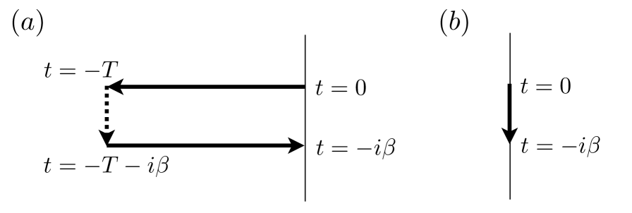
Figure 1: (a) Keldysh contour for real-time diagrammatics. If the time-evolution along the dashed line does not contribute an extra factor, the whole contour can be deformed to one along the imaginary-time from $t=-i\beta$ to $t=0$ as shown in (b).

In this subsection, we discuss conventional arguments of the analytic continuation of a real-time theory to an imaginary-time theory. We furthermore illustrate why such deformation of time-contour fails for a steady-state nonequilibrium, closely following the argument by Doyon and Andrei doyon .

In equilibrium, the thermal average of an observable $\hat{A}$ is given as

$$\langle\hat{A}\rangle=\lim_{T\to\infty}\frac{{\rm Tr}S(0,-T)\hat{\rho}_{0}S(-T,0)\hat{A}}{{\rm Tr}S(0,-T)\hat{\rho}_{0}S(-T,0)},$$ (22)

with the time-evolution operator $S(t_{1},t_{2})=e^{-itH(t_{1}-t_{2})}$ with the full Hamiltonian $\hat{H}$ and the non-interacting density matrix $\hat{\rho}_{0}=e^{-\beta\hat{H}_{0}}$. We consider that the limit $T\to\infty$ exists as discussed in the previous section. In the interaction picture with $\hat{V}_{I}(t)=e^{it\hat{H}_{0}}\hat{V}e^{-it\hat{H}_{0}}$, the above relation can be rewritten as

$$\langle\hat{A}\rangle=\lim_{T\to\infty}\frac{{\rm Tr}S_{I}(0,-T)\hat{\rho}_{0}S_{I}(-T,0)\hat{A}}{{\rm Tr}S_{I}(0,-T)\hat{\rho}_{0}S_{I}(-T,0)},$$ (23)

with

$$S_{I}(t_{1},t_{2})={\cal T}\exp\left[-i\int_{t_{2}}^{t_{1}}ds\hat{V}_{I}(s)\right],$$ (24)

with the time-ordering operator ${\cal T}$ defined as the time moving in the direction $t_{2}\to t_{1}$. Using the relation,

$$S_{I}(b,a)=e^{-icH_{0}}S_{I}(b+c,a+c)e^{icH_{0}},$$ (25)

one can write

$$S_{I}(0,-T)\hat{\rho}_{0}=\hat{\rho}_{0}S_{I}(-i\beta,-i\beta-T),$$ (26)

in the similar manner as Ref. doyon, . Then $\langle\hat{A}\rangle$ is written as

$$\langle\hat{A}\rangle \!\!=\!\! \lim_{T\to\infty}\frac{{\rm Tr}\hat{\rho}_{0}S_{I}(-i\beta,-i\beta-T)S_{I}(-T,0)\hat{A}}{{\rm Tr}\hat{\rho}_{0}S_{I}(-i\beta,-i\beta-T)S_{I}(-T,0)}$$

$$\!\!=\!\! \lim_{T\to\infty}\frac{\langle S_{I}(-i\beta,-i\beta-T)S_{I}(-T,0)\hat{A}\rangle_{0}}{\langle S_{I}(-i\beta,-i\beta-T)S_{I}(-T,0)\rangle_{0}}$$

If we can insert the factor $S_{I}(-i\beta-T,-T)$ [denoted as dashed line in Fig. 1(a)] between $S_{I}(-i\beta,-i\beta-T)$ and $S_{I}(-T,0)$, one can close the time-contour and analytically continue to the contour along the imaginary-time $(0,-i\beta)$ [Fig. 1(b)].

Using the Wick’s theorem and the linked-cluster theorem, the terms contributing to $\langle\hat{A}\rangle$ are of the type

$$\langle V_{I}(s_{1})V_{I}(s_{2})\cdots V_{I}(s_{n})\hat{A}(0)\rangle_{0,{\rm connected}}\;,$$ (28)

where the time $s=0$ and the interaction times $\{s_{1},\cdots,s_{n}\}$ are all interconnected by Wick’s contractions. When the interaction $\hat{V}$ and the observable $\hat{A}$ are operators local to the QD, one can use the relation Eq. (16). We consider a case that one of $s_{k}$ in $\langle V_{I}(s_{1})\cdots V_{I}(s_{n})\hat{A}\rangle_{0,{\rm con}}$ belongs in the interval $[-T,-i\beta-T]$. In its connected Wick’s contractions the operators in $\hat{A}$ may be eventually linked to $s_{k}$ via a forward sequence $\{s^{\prime}_{0}=0,\cdots,s^{\prime}_{p-1},s^{\prime}_{p}=s_{k}\}$ and a backward sequence $\{s^{\prime\prime}_{0}=s_{k},\cdots,s^{\prime\prime}_{q-1},s^{\prime\prime}_{q}=0\}$. For the forward sequence $\{s^{\prime}_{0}=0,\cdots,s^{\prime}_{p-1}\}$ with the times on the real-axis, we can use Eq. (16),

$$e^{-\Gamma\sum_{n=1}^{p-1}|s^{\prime}_{n}-s^{\prime}_{n-1}|}\sim e^{-\Gamma{\rm max}\{|s^{\prime}_{1}|,\cdots,|s^{\prime}_{p-1}|\}}.$$ (29)

Similar expression holds for the backward sequence. For the last term involving $s_{k}\in[-T,-i\beta-T]$, we have a contraction of $\langle d(s^{\prime\prime}_{1})d^{\dagger}(s_{k})\rangle\langle d(s_{k})d^{\dagger}(s^{\prime}_{p-1})\rangle$. For $-\beta<{\rm Im}(s_{k})<0$, the two factors remain finite and give a contribution proportional to $e^{-\Gamma(|T+s^{\prime}_{p-1}|+|T+s^{\prime\prime}_{1}|)}$. Therefore, when one of the interaction events occurs on the contour $[-T,-i\beta-T]$, the corresponding term becomes exponentially small. When traced with local operator $\hat{A}$, the factorization property doyon holds

$$S_{I}(-i\beta,-i\beta-T)S_{I}(-T,0)\to S_{I}(-i\beta,0).$$ (30)

This shows that the Wick rotation between real-time and imaginary-time theory is valid in equilibrium and

$$\langle\hat{A}\rangle=\frac{\langle S_{I}(-i\beta,0)\hat{A}\rangle_{0}}{\langle S_{I}(-i\beta,0)\rangle_{0}}\;\;.$$ (31)

Next we ask whether the same argument can be extended to the steady-state nonequilibrium with the initial density matrix at time $t=-T$ given by $\hat{\rho}_{0}=e^{-\beta(\hat{H}_{0}-\Phi\hat{Y}_{0})}$. In order to move $\hat{\rho}_{0}$ in Eq. (22) to the leftmost position in the trace, we write $\hat{H}=\hat{H}^{\Phi}+\hat{V}^{\Phi}$ with $\hat{H}^{\Phi}_{0}=\hat{H}_{0}-\Phi\hat{Y}_{0}$ and $\hat{V}^{\Phi}=\hat{V}+\Phi\hat{Y}_{0}$. Defining $V^{\Phi}_{I}(t)=e^{it\hat{H}^{\Phi}_{0}}\hat{V}^{\Phi}e^{-it\hat{H}^{\Phi}_{0}}$, we can utilize the same argument as before to write

$$\langle\hat{A}\rangle=\lim_{T\to\infty}\frac{\langle S^{\Phi}_{I}(-i\beta,-i\beta-T)S^{\Phi}_{I}(-T,0)\hat{A}\rangle_{0}}{\langle S^{\Phi}_{I}(-i\beta,-i\beta-T)S^{\Phi}_{I}(-T,0)\rangle_{0}}\;\;.$$ (32)

However, unlike in equilibrium, we cannot use Eq. (16) for a contraction containing $V^{\Phi}_{I}(s)$ since $\hat{V}^{\Phi}=\hat{V}+\Phi\hat{Y}_{0}$ contains spatially extended operators $c^{\dagger}_{\alpha k\sigma}c_{\alpha^{\prime}k^{\prime}\sigma^{\prime}}$ with contributions well away from the QD. Furthermore, $V^{\Phi}_{I}(s)=e^{is\hat{H}^{\Phi}_{0}}\hat{V}e^{-is\hat{H}^{\Phi}_{0}}+\Phi\hat{Y}_{0}$ with a constant of motion $\hat{Y}_{0}$ with respect to $\hat{H}^{\Phi}_{0}$, and $V^{\Phi}_{I}(s)$ would never lead to an exponential decay for the interactions occurring on the dashed contour in FIG. 1(a). This shows that a straightforward analytic continuation of the nonequilibrium Keldysh contour to an imaginary-time one is not possible.

II.4 Matsubara voltage

Recently, one of the authors and Heary prl07 proposed that, by introducing a Matsubara term to the source-drain voltage, one can extend the equilibrium formalism such that the perturbation expansion of the imaginary-time Green function can be mapped to the Keldysh real-time theory. The unperturbed Hamiltonian is written as

$$\hat{K}_{0}(i\varphi_{m})=\hat{H}_{0}+(i\varphi_{m}-\Phi)\hat{Y}_{0},$$ (33)

with the Matsubara voltage $\varphi_{m}=4\pi m/\beta$ with integer $m$. We take the many-body interaction $\hat{V}$ as perturbation.

The non-interacting Hamiltonian appears in the perturbative expansion in two ways: first in the thermal factors $e^{-\beta\hat{K}_{0}}$, and second in the time-evolution $e^{-\tau\hat{K}_{0}}$ for the imaginary-time variable $\tau\in[0,\beta)$. The main trick of this formalism is that in the thermal factor $i\varphi_{m}$-dependence drops out as follows. Since $[\hat{H}_{0},\hat{Y}_{0}]=0$, $e^{-\beta\hat{K}_{0}}=e^{-\beta(\hat{H}_{0}-\Phi\hat{Y}_{0})}e^{-i\varphi_{m}\beta\hat{Y}_{0}}$. Since, with respect to the non-interacting scattering state basis, $\hat{Y}_{0}$ is diagonal and has (half)-integer eigenvalues, $e^{-i\varphi_{m}\beta\hat{Y}_{0}}=1$, and we have the important identity

$$e^{-\beta\hat{K}_{0}(i\varphi_{m})}=e^{-\beta(\hat{H}_{0}-\Phi\hat{Y}_{0})}=\hat{\rho}_{0}\;\;.$$ (34)

Therefore, the equivalence of the imaginary-time and real-time formalism crucially rests on how the double analytic continuation $i\varphi_{m}-\Phi\to 0$ and $\tau\to it$ is performed. Since the $i\varphi_{m}$-dependence in the thermal factor completely drops out, the analytic continuation only concerns the time-evolution. For $\tau\in[0,\beta)$, $e^{-i\varphi_{m}\tau\hat{Y}_{0}}\neq 1$ and $i\varphi_{m}$-dependence does not drop out. Thus, one could argue that as $i\varphi_{m}-\Phi\to 0$ and $\tau\to it$ are taken in that order,

$$e^{-\tau[\hat{H}_{0}+(i\varphi_{m}-\Phi)\hat{Y}_{0}]}\to e^{-\tau\hat{H}_{0}}\to e^{-it\hat{H}_{0}}.$$ (35)

However, as we will point out in detail later, integrals over interaction times may create energy denominators of the type $(K_{n}-K_{m})^{-1}$ in the perturbation expansions, with $K_{n}$ being the $n$-th eigenvalue of $\hat{K}_{0}$. In such cases, the details of the path in the complex plane, along which the analytic continuation $\epsilon_{\varphi}\equiv i\varphi_{m}-\Phi\to\pm i0^{+}$ is taken, become relevant. On the other hand, in the real-time theory, the convergence factor $i\eta$ in the energy denominators determines what poles should be chosen.

III Perturbation expansion

III.1 Real-time expansion

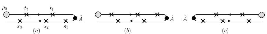
Figure 2: (a) Keldysh contour in forward direction. Crosses mark interaction points $\hat{V}$ and the dot an observable $\hat{A}$. (b) Reversed series of scattering points. (c) Backward Keldysh contour with scattering events equivalent to (a) if $\hat{A}$ is written in terms of QD operators.

In this section, we investigate under what conditions the role of the regularization factor $\eta$ of the time-independent real-time theory becomes unimportant. We assume that a perturbation expansion of Eq. (23) exists. To illustrate the mathematical structure we choose the fifth-order contribution (as shown in FIG. 2) and introduce a spectral representation with respect to the non-interacting scattering state basis. For the particular time-ordering considered in FIG. 2(a), the expression reads

$$S_{a} = (-i)^{5}{\rm Tr}\left[\int_{0}^{-\infty}ds_{3}\int_{0}^{s_{3}}ds_{2}\int_{0}^{s_{2}}ds_{1}\right.$$ (36)

$$\hat{V}_{I}(s_{3})\hat{V}_{I}(s_{2})\hat{V}_{I}(s_{1})\hat{A}$$

$$\left.\int_{-\infty}^{0}dt_{2}\int_{t_{2}}^{0}dt_{1}\hat{V}_{I}(t_{1})\hat{V}_{I}(t_{2})\hat{\rho}_{0}\right].$$

Here we use the notation for intermediate times such that $t_{i}$ are for the forward contour ($-\infty\to 0$, upper time contour) and $s_{i}$ for the backward (lower) contour. We redefine the time as $t_{1}^{\prime}=t_{1}$, $t_{2}^{\prime}=t_{2}-t_{1}$, $t_{i}^{\prime}=t_{i}-t_{i-1}$ etc., and the upper part of the Keldysh contour becomes

$$\int_{-\infty}^{0}dt_{2}\int_{t_{2}}^{0}dt_{1}\hat{V}_{I}(t_{1})\hat{V}_{I}(t_{2})$$

$$= \int_{-\infty}^{0}dt_{2}^{\prime}\int_{-\infty}^{0}dt_{1}^{\prime}\hat{V}_{I}(t_{1}^{\prime})\hat{V}_{I}(t_{1}^{\prime}+t_{2}^{\prime})$$

$$= \int_{-\infty}^{0}dt_{2}^{\prime}\int_{-\infty}^{0}dt_{1}^{\prime}e^{iH_{0}t_{1}^{\prime}}\hat{V}e^{iH_{0}t_{2}^{\prime}}\hat{V}.$$

For a spectral representation with respect to energy eigenstates, we introduce the convergence factor $e^{\eta(t_{1}^{\prime}+t_{2}^{\prime})}$ for the reasons discussed in section IA. Then with respect to the non-interacting Fock basis $|n\rangle$ and $|p\rangle$,

$$(-i)^{2}\langle p|\int_{-\infty}^{0}dt_{2}\int_{t_{2}}^{0}dt_{1}\hat{V}_{I}(t_{1})\hat{V}_{I}(t_{2})|n\rangle=\sum_{q}\frac{V_{pq}V_{qn}}{(E_{n}-E_{p}+i\eta)(E_{n}-E_{q}+i\eta)}\;.$$ (38)

One can do the same for the lower part of the Keldysh contour,

$$(-i)^{3}\langle n|\int_{0}^{-\infty}ds_{3}\int_{0}^{s_{3}}ds_{2}\int_{0}^{s_{2}}ds_{1}\hat{V}_{I}(s_{3})\hat{V}_{I}(s_{2})\hat{V}_{I}(s_{1})|l\rangle =$$ (39)

$$\sum_{mk}\frac{V_{nm}V_{mk}V_{kl}}{(E_{n}-E_{m}-i\eta)(E_{n}-E_{k}-i\eta)(E_{n}-E_{l}-i\eta)}\;.$$

Therefore the above expression $S_{a}$ can be written as

$$S_{a}=\sum_{nmklpq}\frac{V_{nm}V_{mk}V_{kl}}{(E_{n}-E_{m}-i\eta)(E_{n}-E_{k}-i\eta)(E_{n}-E_{l}-i\eta)}A_{lp}\frac{V_{pq}V_{qn}}{(E_{n}-E_{p}+i\eta)(E_{n}-E_{q}+i\eta)}\rho_{n}.$$ (40)

Note that all energy denominators consist of one energy anchored at $|n\rangle$ where $\hat{\rho}_{0}$ acts at $t=-\infty$ and the other energy of intermediate states $|m,k,l,p,q\rangle$. For the forward contour, the state $|n\rangle$ contributes the energy $E_{n}+i\eta$ in the energy denominator, and $E_{n}-i\eta$ for the backward contour.

We now consider a counter-time-ordering as depicted in FIG. 2(b) where the number of scattering events on the lower and upper branches are swapped. After an explicit calculation by applying the same rules as before, one gets

$$S_{b}=\sum_{nmklpq}\frac{V_{nq}V_{qp}}{(E_{n}-E_{q}-i\eta)(E_{n}-E_{p}-i\eta)}A_{pl}\frac{V_{lk}V_{km}V_{mn}}{(E_{n}-E_{l}+i\eta)(E_{n}-E_{k}+i\eta)(E_{n}-E_{m}+i\eta)}\rho_{n}.$$ (41)

Starting with the state $|n\rangle$, the numerator $V_{nq}V_{qp}A_{pl}V_{lk}V_{km}V_{mn}\rho_{n}$ in Eq. (41) represents the reversed process of $\rho_{n}V_{nm}V_{mk}V_{kl}A_{lp}V_{pq}V_{qn}$ in Eq. (40). The factor $\rho_{n}V_{nm}V_{mk}V_{kl}A_{lp}V_{pq}V_{qn}$ is understood as the amplitude of the following process

$$S_{a}: |n\rangle\xrightarrow{\hat{V}}|q\rangle\xrightarrow{\hat{V}}|p\rangle\xrightarrow{\hat{A}}$$ (42)

$$\;\;\;|l\rangle\xrightarrow{\hat{V}}|k\rangle\xrightarrow{\hat{V}}|m\rangle\xrightarrow{\hat{V}}|n\rangle.$$

The many-body interaction can be written in terms of four scattering state operators as $\hat{V}=\sum v_{1234}\psi^{\dagger}_{1}\psi^{\dagger}_{2}\psi_{3}\psi_{4}$. With the on-site Coulomb interaction,

$$\hat{V}=U\sum_{\{\alpha,k\}}t_{1}t_{2}t_{3}t_{4}g^{*}_{1}g_{2}g^{*}_{3}g_{4}\psi^{\dagger}_{1\uparrow}\psi_{2\uparrow}\psi^{\dagger}_{3\downarrow}\psi_{4\downarrow},$$ (43)

where the shorthand notations $t_{i}=t_{\alpha_{i}}/\sqrt{\Omega}$, $g_{i}=g_{d}(k_{i})$ and $\psi^{\dagger}_{i\sigma}=\psi^{\dagger}_{\alpha_{i}k_{i}\sigma}$ have been used. Note that any creation of a particle $\psi^{\dagger}_{i}$ is associated with the factor $t_{i}g^{*}_{i}$, and the annihilation $\psi_{j}$ with $t_{j}g_{j}$. For the observable $\hat{A}$ we consider a one-body operator $\hat{A}=\sum a_{12}\psi^{\dagger}_{1}\psi_{2}$ for simplicity. The operator $\hat{V}$ creates up to two particle-hole pairs of type $\psi$, and for a non-zero matrix element $\langle n|V|m\rangle$, $|n\rangle$ and $|m\rangle$ differ only by up to one particle-hole pair per spin channel. Thus, in the above process Eq. (42), which starts and ends with $|n\rangle$, the product of creation operators $\psi^{\dagger}_{\alpha k\sigma}$ must match the that of annihilation operators $\psi_{\alpha k\sigma}$. Therefore, the matrix element for the process Eq. (42) must be of the form

$$S_{a}:|t_{1}g_{1}|^{2}|t_{2}g_{2}|^{2}\cdots t_{i}g_{i}a_{ij}t_{j}g_{j}^{*}.$$ (44)

Similarly, the process for $S_{b}$-term

$$S_{b} : |n\rangle\xrightarrow{\hat{V}}|m\rangle\xrightarrow{\hat{V}}|k\rangle\xrightarrow{\hat{V}}$$ (45)

$$\;\;\;|l\rangle\xrightarrow{\hat{A}}|p\rangle\xrightarrow{\hat{V}}|q\rangle\xrightarrow{\hat{V}}|n\rangle$$

must contain the same set of $\{\psi^{\dagger},\psi\}$ with the same states, only in the reversed order. The matrix element for the process then becomes

$$S_{b}:|t_{1}g_{1}|^{2}|t_{2}g_{2}|^{2}\cdots t_{j}g_{j}a_{ji}t_{i}g^{*}_{i}.$$ (46)

If the operator $\hat{A}$ satisfies the following property

$$g_{d}(k_{i})a_{ij}[g_{d}(k_{j})]^{*}=g_{d}(k_{j})a_{ji}[g_{d}(k_{i})]^{*},$$ (47)

the matrix elements for counter-contours (a) and (b) match, i.e.

$$V_{nm}V_{mk}V_{kl}A_{lp}V_{pq}V_{qn}=V_{nq}V_{qp}A_{pl}V_{lk}V_{km}V_{mn}.$$ (48)

With this condition, $S_{a}(\eta)=S_{b}(-\eta)$, and $S_{a}+S_{b}$, inside the expression for $\langle\hat{A}\rangle$, is independent of the sign of $\eta$ and has a well-defined limit of $\eta\to\pm 0$. The above argument can be repeated for any order of the perturbation expansion, i.e. the use of a spectral representation is permitted and the result independent of the convergence factor $\eta$ provided that the contour has itself as the counter-contour, $S_{a}(\eta)=S_{a}(-\eta)$.

Which of the physically interesting operators do satisfy the above condition Eq. (47) respectively (48)? It is easy to see that it is true for any operator $\hat{A}$ which is a simple function of $n_{d\sigma}=d^{\dagger}_{\sigma}d_{\sigma}$. A general two-body operator

$$\hat{A}=\sum_{1234}a_{1234}\psi^{\dagger}_{1}\psi^{\dagger}_{2}\psi_{3}\psi_{4}$$

also falls into this class if it satisfies

$$g_{d}(k_{i})g_{d}(k_{j})a_{ijnm}[g_{d}(k_{n})g_{d}(k_{m})]^{*}$$

$$=g_{d}(k_{n})g_{d}(k_{m})a_{nmij}[g_{d}(k_{i})g_{d}(k_{j})]^{*}.$$ (49)

Unfortunately, the current operator Eq. (14) does not satisfy the condition Eq. (47), and a direct analytic continuation is not available, as we will discuss shortly. Therefore, we have to resort to the Meir-Wingreen formula, wingreen which relates the current to the spectral function.

We have so far ignored coinciding energy denominators in the perturbation expansion leading to overlapping $\delta$-functions. For the sake of simplicity we consider a second-order contribution from Eq. (23). By expanding it into different time-orderings, we obtain

$$\int^{T}_{0}dt_{1}\int^{T}_{t_{1}}dt_{2}\hat{\rho}_{0}\hat{V}_{I}(t_{2})\hat{V}_{I}(t_{1})\hat{A}$$

$$+\int_{T}^{0}dt_{1}\int^{T}_{0}dt_{2}\hat{V}_{I}(t_{1})\hat{\rho}_{0}\hat{V}_{I}(t_{2})\hat{A}$$

$$+\int_{T}^{0}dt_{1}\int_{T}^{t_{1}}dt_{2}\hat{V}_{I}(t_{1})\hat{V}_{I}(t_{2})\hat{\rho}_{0}\hat{A}.$$ (50)

We now introduce the convergence factor $e^{\eta t}$ and take $T\to\infty$ to obtain the expression

$$\sum_{nml}\left[\frac{\rho_{n}}{(E_{n}-E_{m}+i\eta)(E_{n}-E_{l}+i\eta)}\right.$$

$$+\frac{\rho_{m}}{(E_{m}-E_{n}+i\eta)(E_{m}-E_{l}-i\eta)}$$

$$\left.+\frac{\rho_{l}}{(E_{l}-E_{n}-i\eta)(E_{l}-E_{m}-i\eta)}\right]V_{nm}V_{ml}A_{ln}.$$

which needs precaution when the two energies in the denominators become equal, because the contribution will be a product of two $\delta$-functions with the same argument. One must be careful when one performs the limit $T\to\infty$. To see this let us go back to the time-dependent description. By keeping $T$ finite, contributions of the form $\delta(E_{n}-E_{m})^{2}$ will actually amount to terms proportional to $T^{2}$ from the integrals. Combining all three integrals we obtain the coefficient to the $T^{2}$-term (i.e. $\delta^{2}$-term) proportional to

$$\begin{array}[b]{ll}\displaystyle\sum_{nml}&(\rho_{n}-2\rho_{m}+\rho_{l})V_{nm}V_{ml}A_{ln}\times\\[8.53581pt] &\displaystyle\delta(E_{n}-E_{m})\delta(E_{m}-E_{l})\end{array}\;\;.$$ (51)

In equilibrium $\rho_{n}=\rho_{m}=\rho_{l}$ for $E_{n}=E_{m}=E_{l}$ and this term vanishes identically. The argument can be easily extended to arbitrary orders in the perturbation expansion.

In the case of nonequilibrium the situation is more complex. Here we discuss in detail what happens to Eq. (51). We consider the case $|n\rangle\neq|m\rangle\neq|l\rangle$, while $E_{n}=E_{m}=E_{l}$. Suppressing the $\delta$-functions, Eq. (51) has the form

$$e^{-\beta E_{n}}(e^{\beta\Phi Y_{0n}}-2e^{\beta\Phi Y_{0m}}+e^{\beta\Phi Y_{0l}})V_{nm}V_{ml}A_{ln}\;.$$

In the matrix element $V_{nm}V_{ml}A_{ln}$, the transition $|n\rangle\to|m\rangle\to|l\rangle\to|n\rangle$ involves a certain series of particle-hole excitations. For instance, $|n\rangle\to|m\rangle$ is given by an exchange of two particle-hole pairs, $\psi^{\dagger}_{\alpha_{1}k_{1}\sigma}\psi_{\alpha_{2}k_{2}\sigma}\psi^{\dagger}_{\alpha_{3}k_{3}\sigma^{\prime}}\psi_{\alpha_{4}k_{4}\sigma^{\prime}}$ in $\hat{V}$, and similarly for $|m\rangle\to|l\rangle$ and $|l\rangle\to|n\rangle$. However, since any creation of $\psi^{\dagger}_{\alpha k\sigma}$ should be matched by $\psi_{\alpha k\sigma}$ only up to 6 indices are independent. Given a particular set of the 6 indices of wave-vectors and spins $\{k_{1}\sigma_{1},k_{2}\sigma_{2},\cdots,k_{6}\sigma_{6}\}$, different permutations of the above 6 pairs of $\{\psi^{\dagger}_{k_{i}\sigma_{i}},\psi_{k_{i}\sigma_{i}}\}$ in $\hat{V}\hat{V}\hat{A}$ determines the matrix element $V_{nm}V_{ml}A_{ln}$. Now, we sum over all possible combinations of reservoir indices $\{\alpha_{1},\cdots,\alpha_{6}\}$ (while keeping the $k$-indices unchanged) for the all twelve $\{\psi^{\dagger},\psi\}$ operators. The matrix element $V_{nm}V_{ml}A_{ln}\propto\prod_{i=1,6}t^{2}_{\alpha_{i}}|g(\epsilon_{k_{i}})|^{2}$. Since the product of $|g(\epsilon_{k_{i}})|^{2}$ are invariant, we collect all possible reservoir weights in $\prod_{i=1,6}t^{2}_{\alpha_{i}}e^{\beta\Phi Y_{0\{n,m,l\}}}$ and each of the three sums in Eq. (51) become the same, i.e. the whole contribution vanishes. A detailed discussion of the mathematics can be found in Appendix A.

In summary, if the observable $\hat{A}$ satisfies Eq. (47), the energy integration in the perturbation expansion can be interpreted as principal-valued, similarly to equilibrium. In Appendix B, we provide as an example the fourth-order contribution to the QD-electrons self-energy and show explicitly that the above properties are satisfied. Since the structures appearing in higher order are of the same type as discussed above, we may actually infer that this property holds in any order of the perturbation expansion.

III.2 Imaginary-time expansion

Unlike the real-time theory, the imaginary-time description is formulated on a finite time interval of $[0,\beta)$, and there is no need for a convergence factor $e^{\eta t}$. Therefore, the energy integrals appearing in the equilibrium theory are always principal-value integrals, which we confirmed in the previous section II.3.

In nonequilibrium, with the imaginary-time effective Hamiltonian $\hat{K}(i\varphi_{m})=\hat{H}_{0}+\epsilon_{\varphi}\hat{Y}_{0}+\hat{V}$ ($\epsilon_{\varphi}=i\varphi_{m}-\Phi$), the thermal average is defined as

$$\langle{\cal A}\rangle=\frac{{\rm Tr}e^{-\beta\hat{K}}{\cal A}}{{\rm Tr}e^{-\beta\hat{K}}}.$$ (52)

The Boltzmann factor can be expanded as

$$e^{-\beta\hat{K}}=e^{-\beta\hat{K}_{0}}{\cal T}_{\tau}\exp\left[-\int_{0}^{\beta}d\tau V_{I}(\tau)\right],$$ (53)

with $V_{I}(\tau)=e^{\tau\hat{K}_{0}}\hat{V}e^{-\tau\hat{K}_{0}}\hat{V}$ and ${\cal T}_{\tau}$ denoting the time-ordering operator for $\tau\in[0\to\beta]$. We consider a second order expansion to understand its mathematical structure,

$${\rm Tr}\,e^{-\beta\hat{K}_{0}}\int_{0}^{\beta}d\tau\int_{0}^{\tau}d\tau^{\prime}V_{I}(\tau)V_{I}(\tau^{\prime})\hat{A}$$ (54)

$$= \int_{0}^{\beta}d\tau\int_{0}^{\tau}d\tau^{\prime}$$

$$\sum_{nml}\rho_{n}e^{\tau(K_{n}-K_{m})}V_{nm}e^{\tau^{\prime}(K_{m}-K_{l})}V_{ml}A_{ln}$$

$$= \sum_{nml}\left[\frac{\rho_{n}}{(K_{n}-K_{m})(K_{n}-K_{l})}\right.$$

$$+\frac{\rho_{m}}{(K_{m}-K_{l})(K_{m}-K_{n})}$$

$$\left.+\frac{\rho_{l}}{(K_{l}-K_{n})(K_{l}-K_{m})}\right]V_{nm}V_{ml}A_{ln}.$$

This expression has the same mathematical structure as in the real-time theory. Even though we considered only one time-ordering in the imaginary-time theory, the upper and lower integral limits in $\int_{0}^{\beta}d\tau\int_{0}^{\tau}d\tau^{\prime}$ combine to create the same permutation of terms as in the real-time theory prl07 .

We have seen earlier that, in the real-time theory, energy denominators can be interpreted as principal-valued since all $\delta$-function contributions from the energy poles vanish. Therefore, if we interpret the energy denominators as principal-valued as $i\varphi_{m}\to\Phi$

$$\frac{1}{K_{n}-K_{m}}\to{\cal P}\left(\frac{1}{E_{n}-E_{m}}\right)$$ (55)

the terms in the imaginary-time theory indeed match those of the real-time approach.

In section IV.1.1, we calculate the double occupancy from continuous-time quantum Monte Carlo method, and numerically verify that the analytic continuation procedure outlined so far works accurately in all orders of perturbation theory as well as for the resummed perturbation series.

III.3 Single-particle self-energy

The analytic properties discussed so far can be used to examine the single-particle self-energy for the Anderson impurity model. The imaginary-time second-order self-energy in the Coulomb interaction $U$ can be written as prl07

$$\Sigma^{(2)}(i\omega_{n},\epsilon_{\varphi})=\sum_{\gamma}\int d\epsilon\frac{\sigma_{\gamma}(\epsilon)}{i\omega_{n}-\frac{\gamma}{2}\epsilon_{\varphi}-\epsilon},$$ (56)

with the spectral function

$$\sigma_{\gamma}(\omega)=U^{2}\left[\prod_{i=1}^{3}\int d\epsilon_{i}A_{0}(\epsilon_{i})\right]\sum_{\alpha_{1}+\alpha_{2}+\alpha_{3}=\gamma}\,\left[f_{1}(1-f_{2})f_{3}+(1-f_{1})f_{2}(1-f_{3})\right]\,\delta(\omega-\epsilon_{1}+\epsilon_{2}-\epsilon_{3})$$ (57)

for the $\gamma$-branch cut ($\gamma=\pm 1,\pm 3$), where

$$A_{0}(\epsilon)=\frac{\Gamma/\pi}{(\epsilon-\epsilon_{0})^{2}+\Gamma^{2}}$$

denotes the non-interacting spectral function of the QD level and $f_{\alpha}=[1+e^{-\beta(\epsilon-\alpha\Phi/2)}]^{-1}$ the Fermi-Dirac factor for the $\alpha$-th reservoir.

Recently, it has been proposed han10 that an inclusion of higher-order contributions will mainly modify the spectral function $\sigma_{\gamma}(\epsilon)$, leading to a $\epsilon_{\varphi}$ dependence like

$$\Sigma(i\omega_{n},\epsilon_{\varphi})=\sum_{\gamma}\int d\epsilon\frac{\sigma_{\gamma}(\epsilon,\epsilon_{\varphi})}{i\omega_{n}-\frac{\gamma}{2}\epsilon_{\varphi}-\epsilon}\;\;.$$ (58)

Based on this expression, one can try to fit $\sigma_{\gamma}(\epsilon,\epsilon_{\varphi})$ to the numerical single-particle self-energy generated from quantum Monte Carlo calculations. However, in order to establish the existence of an analytic continuation limit of the imaginary-time self-energy, one should first show that the real-time self-energy possesses the analytic property discussed in the previous section, namely that the energy poles are principal-valued. The rather lengthy and technical argument is provided in Appendix B for the fourth-order self-energy diagrams. It can be shown explicitly that contributions involving products of $\delta$-functions with identical argument vanish identically, resulting in the necessary analytic properties discussed in the previous section.

Again, investigating the general structures appearing in the perturbation expansion of the self-energy, we are confident that this property indeed holds in any order and also survives the resummation of the series. The latter aspect, however, cannot be proven rigorously, but is strongly supported by the numerical evidence from our Monte-Carlo simulations.

In a recent work by Dirks et al. dirks and a accompanying paper to this work, a general analytic continuation approach based on the multi-variable complex function theory and its double analytic continuation of $(i\omega_{n},i\varphi_{m})$ have been systematically studied.

III.4 Forward and backward steady-state

We have seen in Section III.1 that we need Eq. (48) for any sequence of matrix elements in order to establish the equivalence of the real and imaginary-time theory. In order to close the formal discussions, let us re-examine the complex conjugate of the matrix elements in relation to the forward- and backward-in-time propagation of scattering state density matrix.

Assume that we propagate a non-interacting density matrix $\rho_{0}=\exp[-\beta(H_{0}-\Phi Y_{0})]$ from the initial time $t=-T$ to the present in the forward direction. Then, according to Gell-Mann and Goldberger gellmann , we obtain

$$\hat{\rho}_{out} = \eta\int_{0}^{\infty}e^{-i{\cal L}T}\left(e^{i{\cal L}_{0}T}\hat{\rho}_{0}\right)e^{-\eta T}dT$$ (59)

$$= \eta\int_{0}^{\infty}e^{-i{\cal L}T}\hat{\rho}_{0}e^{-\eta T}dT$$

$$= \frac{\eta}{\eta+i{\cal L}}\hat{\rho}_{0}$$

$$= \hat{\rho}_{0}+\frac{1}{-{\cal L}+i\eta}{\cal L}_{V}\hat{\rho}_{0}\;\;,$$

with ${\cal L}_{V}$ the Liouvillian representing the interaction parts not contained in ${\cal L}_{0}$. $\hat{\rho}_{out}$ is the fully interacting density matrix at $t=0$ and $\hat{\rho}_{0}$ non-interacting density matrix at $t=0$. The meaning of the above equation is that we unwind a non-interacting density matrix to a remote time $t=-T$ and re-evolve it with full interaction to the present time. By taking the average over the remote time $T$, we filter out transient oscillations.

Alternatively, we can also consider a backward propagation of density matrix evolving from the remote future by writing

$$\hat{\rho}_{in} = \eta\int_{0}^{\infty}e^{i{\cal L}T}\left(e^{-i{\cal L}_{0}T}\hat{\rho}_{0}\right)e^{-\eta T}dT$$ (60)

$$= \hat{\rho}_{0}+\frac{1}{-{\cal L}-i\eta}{\cal L}_{V}\hat{\rho}_{0}.$$

If we initially choose $\hat{\rho}_{0}$ as the density matrix of a quantum dot system of disconnected dot and reservoirs, ${\cal L}_{V}={\cal L}_{t}+{\cal L}_{U}$ includes both the hopping to the leads and the Coulomb interaction on the dot. We first construct the scattering states with respect to the hopping, and then with respect to the Coulomb interaction. After the first step, the scattering states become prb07

$$\psi^{\dagger}_{\alpha k\sigma,out} = c^{\dagger}_{\alpha k\sigma}+\frac{t}{\sqrt{\Omega}}g_{d}(k)d^{\dagger}_{\sigma}+\cdots$$ (61)

$$\psi^{\dagger}_{\alpha k\sigma,in} = c^{\dagger}_{\alpha k\sigma}+\frac{t}{\sqrt{\Omega}}g_{d}(k)^{*}d^{\dagger}_{\sigma}+\cdots,$$ (62)

and we can construct respective scattering-state density matrices $\hat{\rho}_{0t,out}$ and $\hat{\rho}_{0t,in}$ with ${\cal L}_{V}={\cal L}_{U}$. The coefficients appearing in front of the dot operators $d^{\dagger}_{\sigma},d_{\sigma}$ etc. for the out and in-scattering states are the complex conjugate of each other. Therefore, the matrix elements of the interaction $\hat{V}=Un_{d\uparrow}n_{d\downarrow}$, written in terms of $\psi_{\alpha k\sigma,\{out,in\}}$-basis, are complex conjugate to each other, i.e. $V_{nm}=V_{\tilde{n}\tilde{m}}^{*}$ (with the tilde denoting the in-scattering basis).

We can now repeat the arguments from Section III.1 for the backward propagation of the density matrix as shown in FIG. 2(c) and find

$$S_{c}=\sum_{nmklpq}\frac{V_{\tilde{n}\tilde{q}}V_{\tilde{q}\tilde{p}}}{(E_{n}-E_{q}+i\eta)(E_{n}-E_{p}+i\eta)}A_{\tilde{p}\tilde{l}}\frac{V_{\tilde{l}\tilde{k}}V_{\tilde{k}\tilde{m}}V_{\tilde{m}\tilde{n}}}{(E_{n}-E_{l}-i\eta)(E_{n}-E_{k}-i\eta)(E_{n}-E_{m}-i\eta)}\rho_{\tilde{n}}.$$

For observables satisfying $A_{nm}=A_{\tilde{n}\tilde{m}}^{*}$, this expression becomes identical to $S_{a}$ in Eq. (40). The same argument holds in any order of the perturbation expansion, and we have ${\rm Tr}\hat{A}\hat{\rho}_{out}={\rm Tr}\hat{A}\hat{\rho}_{in}$ and $\langle\hat{A}\rangle=\frac{1}{2}(\langle\hat{A}\rangle_{out}+\langle\hat{A}\rangle_{in})$. Therefore, from Eqs. (59), (60), we have

$$\langle\hat{A}\rangle = \langle\hat{A}\rangle_{0}+\left\langle\hat{A}\frac{1}{2}\left(\frac{1}{-{\cal L}+i\eta}+\frac{1}{-{\cal L}-i\eta}\right){\cal L}_{V}\hat{\rho}_{0}\right\rangle=\langle\hat{A}\rangle_{0}+\left\langle\hat{A}{\cal P}\left(\frac{1}{-{\cal L}}\right){\cal L}_{V}\hat{\rho}_{0}\right\rangle\;\;,$$ (63)

i.e., the conditions for replacing the energy denominators by their principal-values, as discussed in section III.1, correspond to a measurement protocol where the observable $\hat{A}$ has the same expectation values with respect to the forward- and backward-propagating density matrices.

IV Static Expectation Values

IV.1 Theoretical background

We have shown that steady-state expectation values of certain local observables $\hat{A}$ can be obtained from analytical continuation of expectation values calculated within the imaginary time Matsubara-voltage formalism. As long as we know the analytic structure of these objects, this can be done easily. However, for a model with true two-particle interactions, one eventually has to resort to numerical evaluations, and an analytical continuation in general requires a more involved computational technique. We therefore want to provide in the following a representation which allows the use of standard tools from equilibrium many-body theory.

A numerical method gives $\langle\hat{A}\rangle(i\varphi_{m})$ and let $\langle\hat{A}\rangle(z_{\varphi})$ be its analytic continuation. We may write formally

$$\langle\hat{A}\rangle(z_{\varphi})=\langle\hat{A}\rangle_{\text{const}}+\chi_{A}(z_{\varphi})$$ (64)

where the part $\chi_{A}(z)$ is holomorphic in the upper and lower half plane, with singularities only on the real axis. If one can furthermore show that the $z\chi_{A}(z)$ is non-singular in the limit $z_{\varphi}\to\infty$, one can finally infer that a spectral representation with respect to the jump function on the real axis exists and hence

$$\langle\hat{A}\rangle(i\varphi_{m})=\langle\hat{A}\rangle_{\text{const}}+\int\frac{\varrho_{A}(\varphi)}{(i\varphi_{m}-\Phi)-\varphi}\,\mathrm{d}\varphi\,$$ (65)

Note that the latter property is not necessarily guaranteed and has to be proven individually for each observable.

Once the validity of the representation (65) is established, one only needs to obtain the “spectral function” $\varrho_{A}(\varphi)$. One evident method to calculate the Matsubara voltage data $\langle\hat{A}\rangle(i\varphi_{m})$ for the observable $\hat{A}$ with respect to the effective system with non-hermitian Hamiltonian at Matsubara voltage $i\varphi_{m}$ is via a QMC simulation.dirks For such data with statistical noise, one then typically employs a maximum-entropy approach (MaxEnt).mem The implementation of a MaxEnt estimator for the physical expectation value is rather straightforward. The values for different $i\varphi_{m}$ are truly statistically independent, and only the variance and correlation between imaginary and real parts of a single $i\varphi_{m}$ value play a role. However, one still needs accurate and unbiased measurements of imaginary-voltage data over a large range of $\varphi_{m}$.dirks This latter requirement makes the use of a continuous-time quantum Monte-Carlo (CT-QMC) algorithm mandatory. In particular, the necessary estimation of the constant offset $\langle\hat{A}\rangle_{\text{const}}$ in Eq. (65) is possible only with CT-QMC, because at present no direct measurement algorithm for this quantity is available and one must determine it from the tail of $\langle\hat{A}\rangle(i\varphi_{m})$ by fitting it to

$$\langle\hat{A}\rangle(i\varphi_{m})\stackrel{{\scriptstyle m\to\infty}}{{\to}}\langle\hat{A}\rangle_{\text{const}}+\frac{c_{A}}{i\varphi_{m}}+\frac{\tilde{c}_{A}}{(i\varphi_{m})^{2}}+\cdots\;\;.$$ (66)

In practice, a weighted least-square fit yields reliable values and error bars for $\langle\hat{A}\rangle_{\text{const}}$. Via Gaussian error propagation it is then possible to incorporate the uncertainty of $\langle\hat{A}\rangle_{\text{const}}$ into the covariance matrix of the quantity $\langle\hat{A}\rangle(i\varphi_{m})-\langle\hat{A}\rangle_{\text{const}}$.

In general, the spectral function $\varrho_{A}(\varphi)$ needs not to be positive semidefinite, or show any symmetry relations with respect to $\varphi$. Since on the other hand the MaxEnt method is only applicable for the inference of positive definite functions, a shift function $\varrho_{\text{shift}}(\varphi)$ of the spectral function $\varrho_{A}(\varphi)$ has to be introduced, which makes the to-be-inferred $\varrho_{A}^{\prime}(\varphi)=\varrho_{A}(\varphi)-\varrho_{\text{shift}}(\varphi)$ positive. We also employ a symmetry condition

$$\varrho_{\text{shift}}(\varphi)=\varrho_{\text{shift}}(-\varphi),$$ (67)

because this choice is robust with respect to the physical result

$$\begin{split}\langle\hat{A}\rangle_{\text{phys}}&=\frac{1}{2}\sum_{\alpha=\pm 1}\langle\hat{A}\rangle(\Phi+\alpha i\eta)\\ &=\langle\hat{A}\rangle_{\text{const}}-\mathcal{P}\!\!\!\!\!\!\int\!\!\,\mathrm{d}\varphi\,\frac{\varrho_{A}(\varphi)}{\varphi}.\end{split}$$ (68)

In the following we want to prove that the double occupancy or magnetization obey this constraint, i.e. have a representation, where $\langle\hat{A}\rangle_{\text{const}}$ is a real number, and $\varrho_{A}(\varphi)\in\mathbb{R}$ is a real-valued spectral function.

IV.1.1 Double Occupancy

The double occupancy in Matsubara-voltage representation is defined as

$$D(i\varphi_{m}):=\left\langle n_{d,\uparrow}n_{d,\downarrow}\right\rangle_{K(i\varphi_{m})}\;,$$ (69)

where the expectation value is taken with respect to the $m$-th effective equilibrium system.

We will first show that the representation (65) holds for the double occupancy, i.e. that we have indeed

$$D(i\varphi_{m})=D_{0}+\int\,\mathrm{d}\varphi\,\frac{\varrho_{\text{D}}(\varphi)}{i\varphi_{m}-\Phi-\varphi}.$$ (70)

We restrict the discussion to the case of particle-hole symmetry and symmetric coupling to the leads, $\Gamma_{L}=\Gamma_{R}$. Within the Matsubara-voltage approach, one can – for fixed $i\varphi_{m}$ – employ the standard techniques of equilibrium many-body theory and obtains the standard resultbulla:1998

$$\begin{split}D(i\varphi_{m})=&\langle n_{\uparrow}\rangle\langle n_{\downarrow}\rangle\\ &+\frac{1}{\beta U}\sum_{\omega_{n}}\Sigma(i\varphi_{m};i\omega_{n})G(i\varphi_{m};i\omega_{n})\mathrm{e}^{i\omega_{n}\eta}\;.\end{split}$$ (71)

Due to particle-hole symmetry, we have $\langle n_{\uparrow}\rangle\langle n_{\downarrow}\rangle=1/4$. Furthermore, from the discussion in section III.3 we can infer that at least the Green’s function decays like $1/i\varphi_{m}$ and hence allows for the existence of a spectral representation (70), as long as there is only a single branch cut at $\mathrm{Im}\,z_{\varphi}=0$.

The real-valuedness of spectral function and constant offset remain to be shown. The general relation $G(-i\varphi_{m},-i\omega_{n})^{*}=G(i\varphi_{m},i\omega_{n})$ holds for Green’s function and self-energy. Inserting this into Eq. (71), we find

$$D(-i\varphi_{m})^{*}=D(i\varphi_{m}).$$ (72)

Consequently, the real part of $D(i\varphi_{m})-D(-i\varphi_{m})$ vanishes. Using the symmetric coupling to the leads, we have an invariance of the Green’s function and self-energy under $(i\varphi_{m}-\Phi)\leftrightarrow-(i\varphi_{m}-\Phi)$. As a result, $D_{0}$ is an actual constant which is obtained for both, upper and lower half plane. Due to the symmetry of $\mathrm{Im}\,D(i\varphi_{m})$, $D_{0}$ is real. By inserting the representation (70) into Eq. (72) we also see that $\varrho_{\text{D}}(\omega)$ is real-valued.

For example, let us consider the equilibrium setup, i.e. $\Phi=0$. At half filling and symmetric coupling to the leads, the function

$$\mathrm{Re}\,D_{\Phi=0}(i\varphi_{m}) = \mathrm{Re}\,D_{\Phi=0}(-i\varphi_{m}),$$ (73)

$$\mathrm{Im}\,D_{\Phi=0}(i\varphi_{m}) \equiv 0.$$ (74)

This is compatible with a conventional bosonic spectral representation

$$D_{\Phi=0}(i\varphi_{m})=\int\,\mathrm{d}\varphi\,\frac{\varrho_{D}(\varphi)}{i\varphi_{m}-\varphi}+D_{0},$$ (75)

with an antisymmetric spectral function

$$\varrho_{D}(\varphi)=-\varrho_{D}(-\varphi);\quad\varrho_{D}(\varphi>0)<0$$ (76)

and the offset $D_{0}>0$. Eq. (74) is not evident for asymmetric couplings or off particle-hole symmetry, because here $G_{0}(i\varphi_{m},i\tau)$ is not real.

IV.1.2 Magnetic Susceptibility

An observable which is much more sensitive to the Kondo effect is the magnetization $M:=(\langle n_{\uparrow}\rangle-\langle n_{\downarrow}\rangle)$ in the presence of a magnetic field $B$ in $z$-direction respectively the magnetic susceptibility $\chi=M/B$ of the quantum dot, because it directly probes the spin degree of freedom of the dot electrons. In equilibrium, a strong dependence on the temperature is observed, on the scale of the Kondo temperature.hewson

As for the double occupancy, the validity of a spectral representation

$$M(i\varphi_{m})=M_{0}+\int\,\mathrm{d}\varphi\,\frac{\varrho_{\text{M}}(\varphi)}{i\varphi_{m}-\Phi-\varphi}$$ (77)

can readily be confirmed. Starting from the symmetry $G(-i\varphi_{m},-i\omega_{n})^{*}=G(i\varphi_{m},i\omega_{n})$, one can again show that $M(-i\varphi_{m})^{*}=M(i\varphi_{m})$, and the same arguments apply concerning the interchange $(i\varphi_{m}-\Phi)\leftrightarrow-(i\varphi_{m}-\Phi)$.

IV.2 Numerical effective-equilibrium data

Let us now turn to the discussion of actual numerical data for magnetization and double occupancy from the quantum Monte-Carlo simulations. As the first step, we analyze these data with respect to the auxiliary variable $\varphi_{m}$, and want to argue that they have a physical interpretation with respect to the actual voltage $\Phi$. In particular, the convergence of the numerical procedures described below implies full consistency of the Matsubara-voltage formalism with regard to the numerical data.

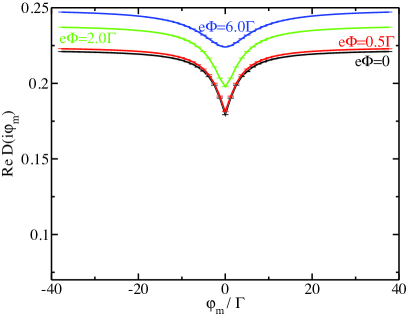
(a) $U=3\Gamma$, $\beta\Gamma=10$

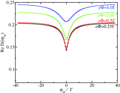
(b) $U=5\Gamma$, $\beta\Gamma=20$

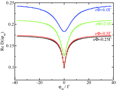
(c) $U=8\Gamma$, $\beta\Gamma=20$

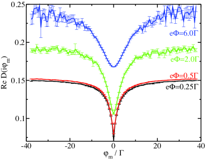
(d) $U=10\Gamma$, $\beta\Gamma=20$

Figure 3: (color online) Real part of the effective-equilibrium double occupancy as a function of the Matsubara voltage $\varphi_{m}$ at several values of interaction strength $U$ and bias voltage $\Phi$.

We find that effective-equilibrium data come along with characteristic energy scales which – after analytic continuation – may translate almost directly into energy scales with respect to the actual source-drain voltage $\Phi$. It is therefore worthwhile to discuss the dependence of the effective-equilibrium expectation values as a function of $\varphi_{m}$ for given physical parameters $\beta$, $U$, and $\Phi$.

Dependence on $\Phi$.

The first thing to notice is that the dependence of the shape of the curves $M(i\varphi_{m})$ and $D(i\varphi_{m})$ on $\Phi$ is rather moderate: for the examples considered, we do not observe any new characteristic energy scales with respect to the Matsubara voltage $\varphi_{m}$ emerging or disappearing as a function of the physical voltage $\Phi$. The most striking influence of $\Phi$ is a change of the offset of the curves $D_{0}$ and $M_{0}$. The offset is changed monotonically as a function of $\Phi$ and cannot explain features such as dips and peaks which are found in the analytically continued data (cf. next section). This is the very reason of our claim that low- to intermediate-energy scales with respect to $\varphi_{m}$ rather directly translate into low- to intermediate-energy scales with respect to $\Phi$, although $\varphi_{m}$ has no direct physical meaning itself.

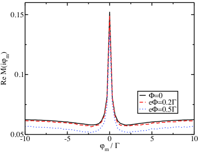
(a) $U=8\Gamma$, $\beta\Gamma=40$, $\mu_{B}B=0.02\Gamma$

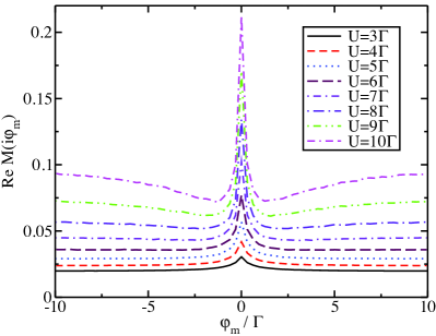
(b) $\beta\Gamma=40$, $\mu_{B}B=0.02\Gamma$, $e\Phi=0.5\Gamma$

Figure 4: (color online) Real part of the effective-equilibrium magnetization as a function of the Matsubara voltage.

Let us substantiate the above statement by the data plotted in Figs. 3 and 4a. In Fig. 3, effective-equilibrium double occupancy curves are shown over a wide range of values of the physical voltage and Coulomb interaction. Each curve exhibits a dip at $\varphi_{m}=0$. As already pointed out above, the dependence on $\Phi$ is rather mild, except for the offset. The same behavior is observed for the magnetization in Fig. 4a, i.e. the voltage $\Phi$ merely introduces an overall shift and a moderate smoothening of the structures.

(a) $U=5\Gamma$

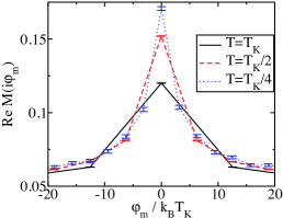
(b) $U=8\Gamma$

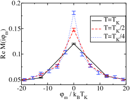
(c) $U=10\Gamma$

Figure 5: (color online) Kondo scaling analysis of effective-equilibrium magnetization data at $\mu_{B}B=T_{K}/2$, $e\Phi=T_{K}/4$. The analysis makes use of the equilibrium Kondo temperatures $k_{B}T_{K}(U=5\Gamma)\approx\frac{1}{10}\Gamma$, $k_{B}T_{K}(U=8\Gamma)\approx\frac{1}{20}\Gamma$, $k_{B}T_{K}(U=10\Gamma)\approx\frac{1}{40}\Gamma$. The latter ratios are chosen to be approximately identical to the results of Haldane’s scaling formula.haldane

Limiting behaviour $\varphi_{m}\to\pm\infty$.

For each $U$ and $\Phi$ a different limit $D_{0}$ is obtained as $\varphi_{m}\to\infty$. If the values $\beta$, $U$, $\Phi$, and in particular $\varphi_{m}$ are large, the effective-equilibrium QMC simulations start to suffer from a significant sign problem. This may result in particularly noisy tails such as the ones for the data with largest $\Phi$ in figure 3d. In these cases, the estimate of $D_{0}$ is subject to much uncertainty and limits the statistical accuracy of physical expectation values.

Dependence on $U$.

As $U$ is increased, the depth of the dips in the double occupancy curves also increases. On the other hand, neither the width nor the shape change significantly. In particular, the emergence of a Kondo scale $T_{\rm K}$ cannot be inferred from these data. Interestingly, for small $U$, the relative contribution of the constant term $D_{0}$ is large compared to the height of the peak which emerges around $\varphi_{m}\approx 0$. As the interaction increases, the central peak becomes more pronounced, and the physical expectation value increasingly depends on the structure of the peak.

For the magnetization in Fig. 4b, a similar picture seems to emerge at first glance, namely a strong increase of the offset $M_{0}$ with $U$ together with a more pronounced peak structure at $\varphi_{m}=0$. The strong increase of both is readily understood as with increasing $U$ the system forms a local moment which is aligns with the external field.

Kondo effect.

Up to now there seems to be no evidence whatsoever for the presence of the Kondo scale $T_{\rm K}$ in the data presented so far. On the other hand, the generation of this many-body scale is usually considered as crucial test for any method proposed for studying the Anderson impurity model. As already pointed out, it is quite apparent from the data in Figs. 3 that $T_{\rm K}$ obviously does not appear to be relevant for this quantity; a fact that is already well known in equilibrium. There the scale $T_{\rm K}$ shows up only in a very indirect way as renormalization of the zero temperature value respectively the scale regulating the approach to it.

The situation is different for the magnetization. Here, the Kondo scale plays a crucial role hewson as it determines the field-strength necessary to break up the Kondo singlet. Hence it must show up in the magnetization; in particular, one must actually expect a scaling behavior with $T_{\rm K}$ for small enough fields. Let us therefore plot the magnetization as function of Matsubara voltage in the form $M(\varphi_{m}/T_{\rm K})$ for values of $U$ beyond the weak-coupling regime for fields and voltages much smaller that the corresponding equilibrium Kondo scales. The result is shown in Fig.  5. Evidently, the width of the peak in the effective-equilibrium magnetization data is nicely scaling with the equilibrium Kondo temperature, i.e. for different values of $U$ the peak structure is essentially left invariant at fixed values of $B$, $\Phi$, and $T$.

IV.3 Results for real voltages

In this section we will introduce the MaxEnt procedure used to infer the spectral functions $\varrho_{D}(\varphi)$ and $\varrho_{M}(\varphi)$ from the effective-equilibrium QMC data. Based on this analytical continuation, we then will discuss the physical results obtained from the auxiliary Matsubara voltage data.

IV.3.1 MaxEnt procedure

Based on the effective-equilibrium data and the exact relation (65), it is in principle possible to uniquely reconstruct the spectral function $\varrho_{A}(\varphi)$ and the offset $\langle\hat{A}\rangle_{\text{const}}$. This is almost completely analogous to the conventional Wick rotation.

However, because in practice a finite set of data is considered, the inversion of equation (65) is no longer unique. On top of this, the quantum Monte-Carlo data are not exact but merely Gaussian random variables. One may easily verify that the noise associated to the variables is amplified by the inversion of equation (65). As a consequence, it will always be possible to find qualitatively very different functions $\varrho_{A}(\varphi)$ which are in agreement with the QMC data. In particular, these functions will yield physically different predictions via equation (68). The problem to obtain physical results from the effective-equilibrium data is thus ill-posed.

Since essentially the same integral equation (65) also relates imaginary-time and real-time properties of conventional Green’s functions, this issue is well-known to the community.mem Although no solution to the problem can be provided, Bayesian inference provides a framework to systematically incorporate a-priori information about a quantity into an estimate. The estimate is most likely with regard to the prior information at hand. The resulting method is called Maximum Entropy (MaxEnt).mem

Let us consider the situation in which the offset $\langle\hat{A}\rangle_{\text{const}}$ has already been determined via a least-square fit. Via error propagation it has been possible to determine the covariance matrix of the quantity $\langle{\hat{A}}\rangle-\langle{\hat{A}}\rangle_{\text{const}}$, i.e. the imaginary-voltage values of the quantity $\chi_{A}(z_{\varphi})$ in equation (64). The remaining task of the MaxEnt is to infer the spectral function $\varrho_{A}(\varphi)$. Let us furthermore assume that the data have been sufficiently transformed with a shift function, such that the function

$$\varrho^{\prime}_{A}(\varphi)=\varrho_{A}(\varphi)-\varrho_{\text{shift}}(\varphi)$$ (78)

is positive (see section IV.1).

The default model for $\varrho^{\prime}_{A}(\varphi)$ is then a positive definite function which in principle should contain features which determine in particular the high-energy behaviour, if known.mem In the case of Green’s functions, perturbation theory or higher-temperature solutions often give good default models.mem In our case, apart from that we used a shift function to construct the positive spectrum, nothing is known about the function, so a flat default model is preferable. As consequence, we use the shift function itself as the default model in the actual computation. For simplicity, let us call the to-be-inferred spectrum $\varrho(\varphi)$ and the default model $\varrho_{\text{def}}(\varphi)$.

On the one hand, the default model gives rise to a relative entropy mem

$$S=\int\,\mathrm{d}\varphi\,\left[\varrho(\varphi)-\varrho_{\text{def}}(\varphi)-\varrho(\varphi)\log\frac{\varrho(\varphi)}{\varrho_{\text{def}}(\varphi)}\right]$$

of the spectral function. On the other hand, the (transformed) effective-equilibrium simulation data with mean values $\bar{a}_{i}$ and covariance $C_{ij}$ yield the measure

$$\chi^{2}=\frac{1}{2}\sum_{i,j}^{N_{QMC}}(\bar{a}_{i}-y_{i})C^{-1}_{ij}(\bar{a}_{j}-y_{j}).$$ (79)

for the quality of the fit. Here $y_{i}$ are the fit values which result from transforming the considered $\varrho(\varphi)$ to the data space, and $N_{QMC}$ is the number of QMC data points $\bar{a}_{i}$. Within the MaxEnt it follows that a functional $Q=\chi^{2}-\alpha S$ must be minimized, where $\alpha>0$ is some hyperparameter.mem

In order to determine $\alpha$, there are several methods, for example the “historic” and the “classic” MaxEnt.mem The former extracts information from the Monte-Carlo data up to the point at which the $\chi^{2}=N_{QMC}$, i.e. the MaxEnt regularization parameter is fixed to the value at which $\chi^{2}=N_{QMC}$. The latter (“classic” MaxEnt) extracts information from QMC data to a larger extent. Based on the probability distribution implied by the default model and maximum-likelihood functionals, a posterior probability of the MaxEnt regularization parameter $\alpha$ is maximized. Because information from the default model is again incorporated rather explicitly, this strategy is particularly good for default models which are close to the actual solution. A rather general feature of “classic” MaxEnt appears to be that the $\chi^{2}$ value of the inferred estimate is generally much smaller than the “historic” value of $N_{QMC}$. Our feeling is that this aspect makes the “classic” estimate more sensitive to statistical fluctuations and vulnerable for over-fitting, but on the same side, the estimate is less biased. A similar increase in fluctuations was pointed out in a recent study.gunnarsson At least if Bayesian evidence coming from the data is weak, the “historic” MaxEnt, on the other hand is more biased towards the default model value, since its estimate is more conservative with regard to the $\chi^{2}$. In our case, the default-model estimate is given by the constant offset $D_{0}$, because our default models are chosen to be even functions with respect to $\varphi$.

As shift functions, wide Gaussians with width $\sigma=\frac{200}{3}\Gamma$ were used, i.e.

$$\varrho_{\text{shift}}(\varphi)=\lambda\cdot\mathrm{e}^{-\varphi^{2}/2\sigma^{2}}.$$ (80)

The amplitude of the functions was varied in such a way that positive functions could be inferred. The different values for differently scaled functions give rise to a certain interval of expectation values, which will be plotted as a result, in the following. An example for the set of inferred functions obtained for a single non-equilibrium system is shown in figure 6.

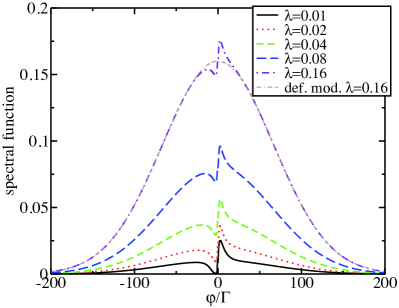
(a) inferred MaxEnt spectra $\varrho_{D}^{\prime}(\varphi)$

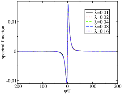
(b) resulting spectral functions $\varrho_{D}(\varphi)$

Figure 6: (color online) MaxEnt inference process for the double occupancy. Parameters are $U=5$, $e\Phi=0.25\Gamma$, $\beta=20\Gamma^{-1}$. Due to lack of prior knowledge, we use a flat default model, i.e. the shift function $\varrho_{\text{shift}}(\varphi)$, see Eq. (80). Remember that the actual spectral function $\varrho_{D}(\varphi)$ was shifted to a positive one, $\varrho_{D}^{\prime}(\varphi)$, via equation (78). One finds that the different equivalent ways of imposing a flat default model for $\varrho_{D}(\varphi)$ yield practically the same spectral function. Nevertheless, computing the physical value (68) yields values which are distributed over a certain range. This range is displayed as error bars in the results plots Figs. 7 and 8.

The left panel shows the actually performed MaxEnt for the shifted spectral functions, using “historic” MaxEnt. Resulting from a flat default model for the function $\varrho_{D}(\varphi)$, the shift function acts as default model here. In this case, choosing a parameter $\lambda<0.01$ yields artifacts in the physical solutions, because the negative regions of $\varrho(\varphi)$ cannot be represented any more. The corresponding actual spectral functions $\varrho(\varphi)$, obtained by subtracting the shift function (80) from the data in the left panel, are shown in the right panel of Fig. 6. The flat default model represents our lack of prior information about the solution and the preference of a smooth solution in case of uncertainty. In general, the different realizations of a flat default model with the shift functions yields almost but not exactly the same spectral functions. In case of limited QMC data quality, it is well knownmem that the usage of a flat default model yields less accurate spectra than an appropriately constructed more informative default model. For example, in case of conventional equilibrium spectral functions of Fermi or Bose systems, a default model should preferably obtain the correct low-order moments, which can often be computed exactly. It can thus be expected that quantities that are calculated from the spectra inferred using the flat default model are biased towards a certain value. Nevertheless, an increase in data quality will eventually reduce the bias of the estimated quantity. We also expect that the precision of our method can be increased by the development of default models which contain additional information like moments. However, at present such type of information is not yet available.

In order to obtain a rough estimate on the error of a physical estimate, we will plot the intervals which are generated by computing the estimates for different values of $\lambda$. Typically, a range from $\lambda=0.01$ to $\lambda=0.16$ is imposed, unless the negative regions of $\varrho(\varphi)$ cannot be represented. For the magnetic susceptibility, the same strategy is used.

IV.3.2 Double occupancy

We will now discuss the analytically continued data of the double occupancy and compare it with respect to zero-temperature second-order perturbation theory.muehlbacher In figure 7 we show double occupancy data for different values of the Coulomb interaction computed with the two different MaxEnt estimators.

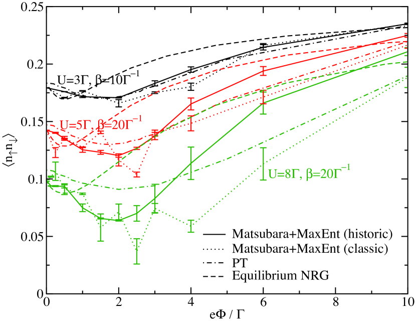
Figure 7: (color online) Double occupancy as a function of the bias voltage at different values of $U$, as compared to second-order perturbation theory. In addition, the dashed lines show the temperature dependence of $\langle n_{\uparrow}n_{\downarrow}\rangle$ in equlibrium as obtained by NRG, assuming $e\Phi=k_{\rm B}T$ (see text).

The complementary behaviour of the two estimators may be well observed in Fig. 7. In the large-bias limit, in which the perturbation theory may be expected to be correct, the classic estimator is closer, and the historic estimate is systematically too high. This is in agreement with our expectation that the historic estimate will be biased from above in case of rather weak Bayesian evidence from QMC data, because the ill-posed continuation problem is particularly severe at high energies.mem Apart from some fluctuations in the “classic” estimator, the same curves are predicted for small voltages. It is important to note that error bars in the figures do not denote statistical errors (which cannot be estimated), but the range of values which a given set of symmetric default models generates.

As compared to the second-order perturbation theory, we find that both methods agree perfectly for interaction strength $U=3\Gamma$. Also both methods predict a minimum in the double occupancy at voltage $e\Phi\approx 2\Gamma$ which slowly shifts to larger values of $\Phi$ and becomes increasingly distinguished as the interaction is increased. There is, however, a clear difference concerning the magnitude of this minimum, which appears much more pronounced in the QMC data as in the perturbation theory. Note that this seems to be the case for both MaxEnt estimators. At present the origin of the deviation is not clear.

One of the issues related to the $\Phi$ dependence of stationary non-equilibrium quantities is to what extent they can be mapped onto an effective equilibrium temperature dependence. To have an idea whether this mapping works, we included in Fig. 7 also the corresponding curves for $\langle n_{\uparrow}n_{\downarrow}\rangle(T)$ as obtained from an NRG equilibrium calculation, assuming $e\Phi=k_{\rm B}T$. Quite apparently, the values at $\Phi\to 0$ nicely coincide, which also tells us that the Matsubara voltage QMC reproduces the proper low bias results even for strong coupling. Note that perturbation theory here deviates systematically with increasing $U$. However, the dependence of $\langle n_{\uparrow}n_{\downarrow}\rangle(\Phi)$ cannot be mapped even qualitatively onto $\langle n_{\uparrow}n_{\downarrow}\rangle(T)$ by a simple ansatz $\Phi\hat{=}\alpha\cdot T$ with some value $\alpha$ for any of the $U$ values considered here. From this observation we would thus conclude that such a mapping is – at least for the simplest possible quantity – not appropriate.

IV.3.3 Magnetic Susceptibility

Similarly, the magnetic susceptibility may be computed as a function of the bias voltage by analytical continuation of the QMC data. As an example, we show the result for $U=8\Gamma$ at the temperature $T=T_{K}/2$ and magnetic field $\mu_{B}B=k_{B}T_{K}/2$

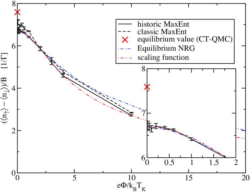
Figure 8: (color online) Magnetic susceptibility as a function of bias voltage in the Kondo regime $U=8\Gamma$ at $\mu_{B}B=k_{B}T_{K}/2$, $T=T_{K}/2$. The dot-dashed line represents an equilibrium NRG calculation for $T\geq T_{\rm K}/2$, rescaled in both magnitude and temperature to match the low-bias behavior of historic MaxEnt (see inset). The double-dot-dash curve finally is a fit of historic MaxEnt to some scaling function (see text).

in Fig. 8. When we compare our continuation results at $\Phi\to 0$ to the exact low-bias limit (i.e. the equilibrium value, displayed as a cross in Fig. 8), the historic MaxEnt is again more strongly biased than the classic MaxEnt, i.e. the deviation from the equilibrium value is stronger. With insufficient QMC information, the outcome is more biased towards the flat default model and from Eq. (68) the integral vanishes in such limit. The constant offset $M_{0}$ lies below the actual physical limit, and therefore, as QMC quality improves, our estimate approaches the correct limit from below. Again, the classic MaxEnt is subject to stronger fluctuations.

In physical terms, the decay in magnetic susceptibility is because of the destruction of the Kondo effect due to the decoherence introduced by the bias voltage. This is in principle similar to the equilibrium behaviour found as a function of temperature.hewson The scale on which the decay of the magnetization takes place appears to be already visible within the imaginary-voltage data shown in Fig. 5b. Apparently, this is due to the rather weak voltage-dependence of imaginary-voltage data (cf. figure 4a). Voltages above $10k_{B}T_{K}$ were not accessible to the MaxEnt, due to a strong sign problem occurring for the QMC simulations of the effective-equilibrium systems associated to the high-$\varphi_{m}$ tails.

We again may compare the voltage dependence of the stationary non-equilibrium magnetization to the temperature dependence in equilibrium. Since we here are at a finite temperature $T=T_{\rm K}/2$, hence the magnetization is smaller than the value at $T=0$, the natural thing to look at is the curve $M(T)\cdot[M(T_{\rm K}/2)/M(0)]$ and rescale temperature with an appropriate factor. The result is shown as dot-dashed line in Fig. 8. Although one can reach a reasonable match for low voltages, a significant deviation occurs already at moderate bias. Thus there does not seem to exist a simple mapping $\Phi\to T$ which will bring the curves to overlap, .i.e. it again seems doubtful that one can describe the effect of finite bias voltage by an effective temperature scale, at least beyond small bias voltages of the order of the Kondo scale.

On the other hand, a rather good account for all data can be achieved by the very simple ansatz

$$\frac{m(\Phi)}{B} \approx \frac{a}{B}\frac{1}{\frac{\tilde{\Phi}^{2}}{\sqrt{b^{2}+\tilde{\Phi}^{2}}}+c}$$

where $\tilde{\Phi}:=\Phi/(2T_{\rm K})$. The result of this fit with $a=0.52$, $b\approx 2$ and $c\approx 3$ is shown as the double-dot-dash curve in Fig. 8. Note that this formula gives the right behavior in the two limits $\Phi\to 0$, viz $M/B\propto 1-c\tilde{\Phi}^{2}$ with some numerical constant $c$, and $\Phi\to\infty$, viz $M/B\propto 1/\Phi$. From scaling analysisrosch one would expect that, in particular for large bias, additional logarithmic corrections appear. Due to the limited data space available we are of course not able to resolve those; furthermore, it is not clear if these logarithmic corrections will actually be visible in the intermediate coupling regime studied here, due to residual charge fluctuations. We therefore view the above formula as a reasonable description in the regime of bias, temperature and field of the order of the Kondo temperature for the intermediate coupling regime of the SIAM.

V Summary

The present paper presents a detailed study on how the imaginary-voltage formalism proposed in Ref. prl07, relates to Keldysh theory. Using series resummations, we are able to show up to all orders that static expectation values of observables, which satisfy certain symmetry relations with respect to the Keldysh contour, map exactly onto the corresponding expressions in Keldysh perturbation theory. In particular, it was pointed out that in order to obtain a physical expectation value, the limiting process $i\varphi_{m}\to\Phi$ has to be taken as principal-value. This prescription ensures, that one generates the principal-value integrals which emerge in the proper real-time theory. For dynamical correlation functions, this was shown explicitly up to fourth order of perturbation theory.

As one important novel result of the present paper we were able to provide an exact spectral representation for static expectation values similar to a Lehmann representation. Based on the representation, using unbiased numerical data from continuous-time quantum Monte-Carlo simulations, we found that the evaluation of the limiting procedure as principal-value expression does indeed give real numbers as physical expectation values. Consequently, the theory is found to be fully consistent in this respect beyond the perturbation arguments given. The double occupancy as function of bias voltage computed this way shows features similar to straight-forward second-order perturbation theory, but we find them to be more pronounced. For the magnetic susceptibility we were able to give numerical estimates on the destruction of the Kondo effect. A comparison to equilibrium NRG shows that the dependence on bias voltage for both, the double occupancy and the magnetic susceptibility, cannot be explained by a simple effective-temperature interpretation.

VI Acknowledgments

We acknowledge valuable discussions with M. Jarrell, J. Freericks, F.B. Anders, S. Schmitt, K. Schönhammer, A. Schiller. AD acknowlegdes financial support by the DAAD through the PPP exchange program, and JH acknowledges the National Science Foundation with the Grant number DMR-0907150, TP the German Science Foundation through SFB 602. AD and TP would also like to acknowledge computer support by the HLRN, the GWDG and the GOEGRID initiative of the University of Göttingen. Parts of the implementation are based on the ALPS 1.3 library alps .

Appendix A Cancellation of overlapping $\delta$-functions in Eq. (51)

With a set of $\{\psi^{\dagger}_{\alpha_{i}k_{i}\sigma_{i}},\psi_{\alpha_{i}k_{i}\sigma_{i}};i=1,\cdots,6\}$ appearing for the matrix elements in Eq. (51), we categorize the thermal factor $e^{\beta\Phi Y_{0\{n,m,l\}}}$ as follows. (i) If $Y_{0n}=Y_{0m}=Y_{0l}$, Eq. (51) vanishes. (ii) If only one of $Y_{0n},Y_{0m},Y_{0l}$ is different from others, $(Y_{0n},Y_{0m},Y_{0l})\in\{(Y_{0},Y_{0},Y_{0}+1),(Y_{0}+1,Y_{0},Y_{0}),(Y_{0},Y_{0}+1,Y_{0}),(Y_{0},Y_{0},Y_{0}+2),(Y_{0}+2,Y_{0},Y_{0}),(Y_{0},Y_{0}+2,Y_{0})\}$ for some reference value $Y_{0}$. If we take the case of $(Y_{0n},Y_{0m},Y_{0l})=(Y_{0},Y_{0},Y_{0}+1)$, the terms contributing for the matrix elements $V_{nm}$, $V_{ml}$ and $A_{ln}$ are from $\psi^{\dagger}_{\tilde{\alpha}_{1}\tilde{k}_{1}}\psi^{\dagger}_{\tilde{\alpha}_{2}\tilde{k}_{2}}\psi_{\tilde{\alpha}_{3}\tilde{k}_{3}}\psi_{\tilde{\alpha}_{4}\tilde{k}_{4}}$, $\psi^{\dagger}_{Rk_{1}}\psi_{Lk_{2}}\psi^{\dagger}_{\tilde{\alpha}_{5}\tilde{k}_{5}}\psi_{\tilde{\alpha}_{6}\tilde{k}_{6}}$, and $\psi^{\dagger}_{Lk_{2}}\psi_{Rk_{1}}\psi^{\dagger}_{\tilde{\alpha}_{7}\tilde{k}_{7}}\psi_{\tilde{\alpha}_{8}\tilde{k}_{8}}$, respectively, where $(\tilde{k}_{1},\cdots,\tilde{k}_{8})$ is a some permutation of $(k_{3},k_{3},k_{4},k_{4},\cdots,k_{6},k_{6})$. The reservoir indices should be chosen such that $\tilde{\alpha}_{5}=\tilde{\alpha}_{6}$ and $\tilde{\alpha}_{7}=\tilde{\alpha}_{8}$, and $(\tilde{\alpha}_{1},\tilde{\alpha}_{2},\tilde{\alpha}_{3},\tilde{\alpha}_{4})$ should satisfy $Y_{0n}=Y_{0m}$. The $\tilde{\alpha}_{i}$ indices are summed over for $L/R$. Then the term in Eq. (51) becomes proportional to

$$(t_{L}t_{R})^{2}(t_{L}^{2}+t_{R}^{2})^{4}\prod_{i=1,6}|g(k_{i})|^{2}e^{\beta\Phi Y_{0}}(1-2+e^{\beta\Phi}).$$

For other combinations of $(Y_{0n},Y_{0m},Y_{0l})=(Y_{0},Y_{0}+1,Y_{0}),(Y_{0}+1,Y_{0},Y_{0})$ the thermal factor becomes $(1-2e^{\beta\Phi}+1)$ and $(e^{\beta\Phi}-2+1)$, respectively, and all three contributions sum up to zero. With the case of $(Y_{0},Y_{0},Y_{0}+2)$, the contribution becomes $(t_{L}t_{R})^{4}(t_{L}^{2}+t_{R}^{2})^{2}\prod_{i=1,6}|g(k_{i})|^{2}e^{\beta\Phi Y_{0}}(1-2+e^{2\beta\Phi})$. The other terms have factors of $(1-2e^{2\beta\Phi}+1),(e^{2\beta\Phi}-2+1)$, and these sum up to zero again.

(iii) When all of $Y_{0n},Y_{0m},Y_{0l}$ are different, $(Y_{0n},Y_{0m},Y_{0l})$ is a permutation of $(Y_{0},Y_{0}+1,Y_{0}+2)$. Since $\hat{V},\hat{A}$ are at most two-particle operators the difference of $Y$-values between states cannot be greater than two. If $(Y_{0n},Y_{0m},Y_{0l})=(Y_{0},Y_{0}+1,Y_{0}+2)$, the factor in Eq. (51) becomes proportional to

$$(t_{L}t_{R})^{4}(t_{L}^{2}+t_{R}^{2})^{2}\prod_{i=1,6}|g(k_{i})|^{2}e^{\beta\Phi Y_{0}}(1-2e^{\beta\Phi}+e^{2\beta\Phi}).$$

Permuting $(Y_{0},Y_{0}+1,Y_{0}+2)$ the sum of the thermal factors can be easily shown to be zero.

Appendix B Fourth order expansion of electron self-energy

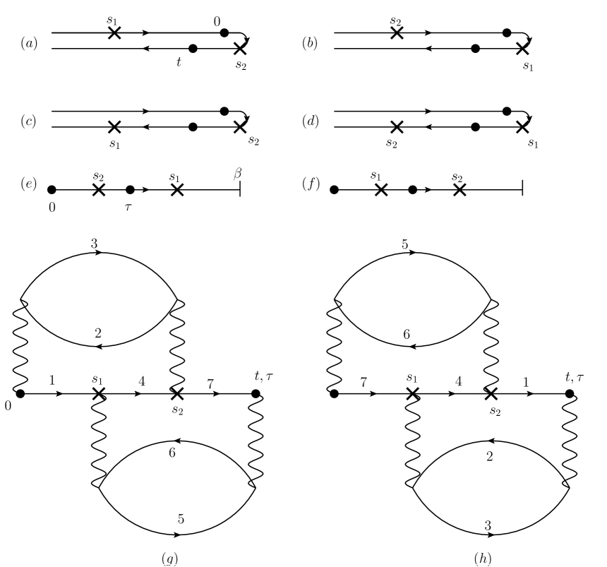
Figure 9: (a-d) Real-time Keldysh contour for self-energy $\Sigma_{(4)}^{>}(t,0)$ in the fourth order perturbation when one intermediate time is in the finite interval $[0,t]$ and the other time in along the contour stretching to $-\infty$. The Wick’s contraction is taken as shown in (g-h). The dummy label of (g) is used for time-orderings (a,c,e) and (h) used for (b,d,f). The cross represents the intermediate times $s_{1}$ and $s_{2}$ for interaction, in addition to the creation/annihilation points $0$ and $t$.

We investigate the energy-pole structure in the real-time perturbation expansion to verify that the $\delta$-function residue disappears and the energy denominators can be interpreted as principal-valued. In the following we consider the perturbation expansion for the self-energy in the fourth order of Coulomb parameter $U$, $\Sigma_{(4)}^{>}(t,0)$ according to the time-orderings along the Keldysh contour, FIG. 9(a-d). Different types of time-orderings will be considered shortly. These time-orderings have one of the intermediate time (marked as cross) within a finite time-interval fixed by time at $0$ and $t$. Given a time-ordering, a particular Wick’s contraction should be chosen. The chosen Wick’s contraction is according to the diagrams in (g-h) which correspond to the most non-trivial vertex correction.

We can evaluate each contribution as follows.

$$S_{a} = f_{1}f_{2}\bar{f}_{3}\bar{f}_{4}\bar{f}_{5}f_{6}\bar{f}_{7}\int_{-\infty}^{0}ds_{1}\int_{0}^{t}ds_{2}e^{-i(\epsilon_{1}-\epsilon_{4}-\epsilon_{5}+\epsilon_{6}-i\eta)s_{1}-i(-\epsilon_{2}+\epsilon_{3}+\epsilon_{4}-\epsilon_{7})s_{2}-i(\epsilon_{5}-\epsilon_{6}+\epsilon_{7})t}$$ (81)

$$S_{b} = \bar{f}_{1}f_{2}\bar{f}_{3}f_{4}f_{5}\bar{f}_{6}\bar{f}_{7}\int_{-\infty}^{0}ds_{2}\int_{0}^{t}ds_{1}e^{-i(\epsilon_{2}-\epsilon_{3}-\epsilon_{4}+\epsilon_{7})s_{1}-i(-\epsilon_{1}+\epsilon_{4}+\epsilon_{5}-\epsilon_{6}-i\eta)s_{2}-i(\epsilon_{1}-\epsilon_{2}+\epsilon_{3})t}$$ (82)

$$S_{c} = \bar{f}_{1}f_{2}\bar{f}_{3}f_{4}f_{5}\bar{f}_{6}\bar{f}_{7}\int_{t}^{-\infty}ds_{1}\int_{0}^{t}ds_{2}e^{-i(\epsilon_{1}-\epsilon_{4}-\epsilon_{5}+\epsilon_{6}-i\eta)s_{1}-i(-\epsilon_{2}+\epsilon_{3}+\epsilon_{4}-\epsilon_{7})s_{2}-i(\epsilon_{5}-\epsilon_{6}+\epsilon_{7})t}$$ (83)

$$S_{d} = f_{1}f_{2}\bar{f}_{3}\bar{f}_{4}\bar{f}_{5}f_{6}\bar{f}_{7}\int_{t}^{-\infty}ds_{2}\int_{0}^{t}ds_{1}e^{-i(\epsilon_{2}-\epsilon_{3}-\epsilon_{4}+\epsilon_{7})s_{1}-i(-\epsilon_{1}+\epsilon_{4}+\epsilon_{5}-\epsilon_{6}-i\eta)s_{2}-i(\epsilon_{1}-\epsilon_{2}+\epsilon_{3})t}.$$ (84)

In these shorthand notation (as discussed in the main text), we omitted the expression $U^{4}[\prod_{i}\int d\epsilon_{i}|g_{d}(\epsilon_{i})|^{2}]$ which is common to all $S_{i}$ terms. $f_{i}=[1+e^{\beta(\epsilon_{i}-\alpha_{i}\Phi/2)}]^{-1}$ and $\bar{f}_{i}=1-f_{i}$. After some algebra, we get

$$S_{a}+S_{d}=-\frac{2f_{1}f_{2}\bar{f}_{3}\bar{f}_{4}\bar{f}_{5}f_{6}\bar{f}_{7}}{(-\epsilon_{2}+\epsilon_{3}+\epsilon_{4}-\epsilon_{7})(\epsilon_{1}-\epsilon_{4}-\epsilon_{5}+\epsilon_{6})}[e^{-i(-\epsilon_{2}+\epsilon_{3}+\epsilon_{4}+\epsilon_{5}-\epsilon_{6})t}-e^{-i(\epsilon_{5}-\epsilon_{6}+\epsilon_{7})t}].$$ (85)

The exponential terms cancel each other at the energy poles and $(\epsilon_{2}-\epsilon_{3}-\epsilon_{4}+\epsilon_{7})^{-1}$ and $(\epsilon_{1}-\epsilon_{4}-\epsilon_{5}+\epsilon_{6})^{-1}$ give well-defined principal-valued integral. This is a typical behavior since an integral within a finite interval $(0,t)$ does not need the convergence factor $e^{\eta t}$ and, accordingly, principal-valued integral is enough. The same can be said for the combination $S_{b}+S_{c}$.

Now, we take the imaginary-time contours in FIG. 9(e-f). After straightforward calculations, we have ($\tilde{\epsilon}_{i}=\epsilon_{i}-\alpha_{i}\epsilon_{\varphi}/2$)

$$S_{e} = f_{1}f_{2}\bar{f}_{3}\bar{f}_{4}\bar{f}_{5}f_{6}\bar{f}_{7}\frac{e^{-(-\tilde{\epsilon}_{2}+\tilde{\epsilon}_{3}+\tilde{\epsilon}_{4}+\tilde{\epsilon}_{5}-\tilde{\epsilon}_{6})\tau}-e^{-(\tilde{\epsilon}_{5}-\tilde{\epsilon}_{6}+\tilde{\epsilon}_{7})\tau}}{(\tilde{\epsilon}_{1}-\tilde{\epsilon}_{4}-\tilde{\epsilon}_{5}+\tilde{\epsilon}_{6})(-\tilde{\epsilon}_{2}+\tilde{\epsilon}_{3}+\tilde{\epsilon}_{4}-\tilde{\epsilon}_{7})}$$ (87)

$$-\bar{f}_{1}f_{2}\bar{f}_{3}f_{4}f_{5}\bar{f}_{6}\bar{f}_{7}\frac{e^{-(\tilde{\epsilon}_{1}-\tilde{\epsilon}_{2}+\tilde{\epsilon}_{3})\tau}-e^{-(\tilde{\epsilon}_{1}-\tilde{\epsilon}_{4}+\tilde{\epsilon}_{7})\tau}}{(\tilde{\epsilon}_{1}-\tilde{\epsilon}_{4}-\tilde{\epsilon}_{5}+\tilde{\epsilon}_{6})(-\tilde{\epsilon}_{2}+\tilde{\epsilon}_{3}+\tilde{\epsilon}_{4}-\tilde{\epsilon}_{7})}.$$

Here (87) corresponds to $S_{a}$ of (81) and (87) to $S_{c}$ of (83). Similarly for $S_{f}$,

$$S_{f} = \bar{f}_{1}f_{2}\bar{f}_{3}f_{4}f_{5}\bar{f}_{6}\bar{f}_{7}\frac{e^{-(\tilde{\epsilon}_{1}-\tilde{\epsilon}_{4}+\tilde{\epsilon}_{7})\tau}-e^{-(\tilde{\epsilon}_{1}-\tilde{\epsilon}_{2}+\tilde{\epsilon}_{3})\tau}}{(\tilde{\epsilon}_{1}-\tilde{\epsilon}_{4}-\tilde{\epsilon}_{5}+\tilde{\epsilon}_{6})(-\tilde{\epsilon}_{2}+\tilde{\epsilon}_{3}+\tilde{\epsilon}_{4}-\tilde{\epsilon}_{7})}$$ (89)

$$-f_{1}f_{2}\bar{f}_{3}\bar{f}_{4}\bar{f}_{5}f_{6}\bar{f}_{7}\frac{e^{-(\tilde{\epsilon}_{5}-\tilde{\epsilon}_{6}+\tilde{\epsilon}_{7})\tau}-e^{-(-\tilde{\epsilon}_{2}+\tilde{\epsilon}_{3}+\tilde{\epsilon}_{4}+\tilde{\epsilon}_{5}-\tilde{\epsilon}_{6})\tau}}{(\tilde{\epsilon}_{1}-\tilde{\epsilon}_{4}-\tilde{\epsilon}_{5}+\tilde{\epsilon}_{6})(-\tilde{\epsilon}_{2}+\tilde{\epsilon}_{3}+\tilde{\epsilon}_{4}-\tilde{\epsilon}_{7})}.$$

At the energy poles at for $\epsilon_{\varphi}\to i\eta$, $S_{f}$ becomes identical to $S_{e}$. Similarly to the real-time diagrams, $(-\tilde{\epsilon}_{2}+\tilde{\epsilon}_{3}+\tilde{\epsilon}_{4}-\tilde{\epsilon}_{7})^{-1}$ has a well-defined principal-value integral regardless of the sign of $\eta$. Therefore for diagrams $S_{a}-S_{f}$ we have correct analytic continuation of imaginary-time results to those of the real-time via

$$\frac{1}{\tilde{\epsilon}_{1}-\tilde{\epsilon}_{4}-\tilde{\epsilon}_{5}+\tilde{\epsilon}_{6}}\to{\cal P}\left(\frac{1}{\epsilon_{1}-\epsilon_{4}-\epsilon_{5}+\epsilon_{6}}\right).$$ (90)

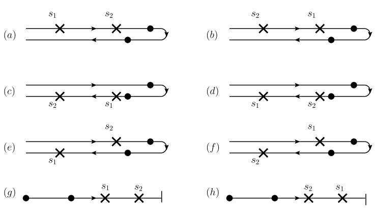
Figure 10: Different time-ordering with two intermediate interaction events extend to infinity. (a,d,e,g) use the label in FIG.1(g) and (b,c,f,h) FIG.1(h).

In FIG. 10, we consider the remaining time-orderings with the two intermediate interaction points extending to infinity. These are harder to deal with, as we discuss below, since the energy poles may overlap.

$$D_{a} = f_{1}\bar{f}_{2}f_{3}\bar{f}_{4}\bar{f}_{5}f_{6}\bar{f}_{7}\iint\displaylimits_{-\infty}^{0}ds_{1}ds_{2}e^{-i(\epsilon_{1}-\epsilon_{4}-\epsilon_{5}+\epsilon_{6}-i\eta)s_{1}-i(\epsilon_{1}-\epsilon_{2}+\epsilon_{3}-\epsilon_{5}+\epsilon_{6}-\epsilon_{7}-i\eta)s_{2}-i(\epsilon_{5}-\epsilon_{6}+\epsilon_{7})t}$$ (91)

$$D_{b} = -\bar{f}_{1}f_{2}\bar{f}_{3}f_{4}f_{5}\bar{f}_{6}f_{7}\int e^{-i(-\epsilon_{1}+\epsilon_{2}-\epsilon_{3}+\epsilon_{5}-\epsilon_{6}+\epsilon_{7}-i\eta)s_{1}-i(-\epsilon_{1}+\epsilon_{4}+\epsilon_{5}-\epsilon_{6}-i\eta)s_{2}-i(\epsilon_{1}-\epsilon_{2}+\epsilon_{3})t}$$ (92)

$$D_{c} = f_{1}\bar{f}_{2}f_{3}\bar{f}_{4}\bar{f}_{5}f_{6}\bar{f}_{7}\int e^{-i(-\epsilon_{1}+\epsilon_{2}-\epsilon_{3}+\epsilon_{5}-\epsilon_{6}+\epsilon_{7}-i\eta)s_{1}-i(-\epsilon_{1}+\epsilon_{4}+\epsilon_{5}-\epsilon_{6}-i\eta)s_{2}-i(\epsilon_{5}-\epsilon_{6}+\epsilon_{7})t}$$ (93)

$$D_{d} = -\bar{f}_{1}f_{2}\bar{f}_{3}f_{4}f_{5}\bar{f}_{6}f_{7}\int e^{-i(\epsilon_{1}-\epsilon_{4}-\epsilon_{5}+\epsilon_{6}-i\eta)s_{1}-i(\epsilon_{1}-\epsilon_{2}+\epsilon_{3}-\epsilon_{5}+\epsilon_{6}-\epsilon_{7}-i\eta)s_{2}-i(\epsilon_{1}-\epsilon_{2}+\epsilon_{3})t}$$ (94)

$$D_{e} = -\bar{f}_{1}\bar{f}_{2}f_{3}f_{4}f_{5}\bar{f}_{6}\bar{f}_{7}\int e^{-i(\epsilon_{1}-\epsilon_{4}-\epsilon_{5}+\epsilon_{6}-i\eta)s_{1}-i(-\epsilon_{2}+\epsilon_{3}+\epsilon_{4}-\epsilon_{7}-i\eta)s_{2}-i(\epsilon_{1}-\epsilon_{4}+\epsilon_{7})t}$$ (95)

$$D_{f} = f_{1}f_{2}\bar{f}_{3}\bar{f}_{4}\bar{f}_{5}f_{6}f_{7}\int e^{-i(\epsilon_{2}-\epsilon_{3}-\epsilon_{4}+\epsilon_{7}-i\eta)s_{1}-i(-\epsilon_{1}+\epsilon_{4}+\epsilon_{5}-\epsilon_{6}-i\eta)s_{2}-i(-\epsilon_{2}+\epsilon_{3}+\epsilon_{4}+\epsilon_{5}-\epsilon_{6})t}$$ (96)

After integrals over $s_{1}$ and $s_{2}$ it is easy to see that $D_{a}(i\eta)=D_{c}(-i\eta)$ and $D_{b}(i\eta)=D_{d}(-i\eta)$. For $D_{e}$ and $D_{f}$, we can swap the dummy indices as $1\leftrightarrow 7$, $2\leftrightarrow 6$, and $3\leftrightarrow 5$, and it becomes $D_{e}(i\eta)=D_{e}(-i\eta)$ and $D_{f}(i\eta)=D_{f}(-i\eta)$. Therefore, we obtain the desired result as (90),

$$\sum_{k=a,\cdots,f}D_{k}(i\eta)=\sum_{k}D_{k}(-i\eta)=\sum_{k}{\cal P}D_{k}(\pm i\eta).$$ (97)

In deriving these relations, no assumptions of $L/R$ and particle-hole symmetry have been used. One can rewrite $D_{a}$ as

$$D_{a}=f_{1}\bar{f}_{2}f_{3}\bar{f}_{4}\bar{f}_{5}f_{6}\bar{f}_{7}\frac{e^{-i(\epsilon_{5}-\epsilon_{6}+\epsilon_{7})t}}{\epsilon_{2}-\epsilon_{3}-\epsilon_{4}+\epsilon_{7}}\left[\frac{1}{\epsilon_{1}-\epsilon_{2}+\epsilon_{3}-\epsilon_{5}+\epsilon_{6}-\epsilon_{7}-i\eta}-\frac{1}{\epsilon_{1}-\epsilon_{4}-\epsilon_{5}+\epsilon_{6}-i\eta}\right].$$ (98)

Here the $+i\eta$ in the denominator will be cancelled by $D_{c}$ and all fractions can be written as principal-valued, unless the poles coincide.

We can now turn to the imaginary-time diagrams FIG. 10(g,h).

$$D_{g} = \frac{f_{1}\bar{f}_{2}f_{3}\bar{f}_{4}\bar{f}_{5}f_{6}\bar{f}_{7}}{-(\tilde{\epsilon}_{2}-\tilde{\epsilon}_{3}-\tilde{\epsilon}_{4}+\tilde{\epsilon}_{7})}\left(-\frac{1}{\tilde{\epsilon}_{1}-\tilde{\epsilon}_{2}+\tilde{\epsilon}_{3}-\tilde{\epsilon}_{5}+\tilde{\epsilon}_{6}-\tilde{\epsilon}_{7}}+\frac{1}{\tilde{\epsilon}_{1}-\tilde{\epsilon}_{4}-\tilde{\epsilon}_{5}+\tilde{\epsilon}_{6}}\right)e^{-(\tilde{\epsilon}_{5}-\tilde{\epsilon}_{6}+\tilde{\epsilon}_{7})\tau}$$ (99)

$$-\frac{\bar{f}_{1}f_{2}\bar{f}_{3}\bar{f}_{4}f_{5}\bar{f}_{6}f_{7}}{(\tilde{\epsilon}_{2}-\tilde{\epsilon}_{3}-\tilde{\epsilon}_{4}+\tilde{\epsilon}_{7})}\frac{e^{-(\tilde{\epsilon}_{1}-\tilde{\epsilon}_{2}+\tilde{\epsilon}_{3})\tau}}{(\tilde{\epsilon}_{1}-\tilde{\epsilon}_{2}+\tilde{\epsilon}_{3}-\tilde{\epsilon}_{5}+\tilde{\epsilon}_{6}-\tilde{\epsilon}_{7})}+\frac{\bar{f}_{1}\bar{f}_{2}f_{3}f_{4}f_{5}\bar{f}_{6}\bar{f}_{7}}{(\tilde{\epsilon}_{2}-\tilde{\epsilon}_{3}-\tilde{\epsilon}_{4}+\tilde{\epsilon}_{7})}\frac{e^{-(\tilde{\epsilon}_{1}-\tilde{\epsilon}_{4}+\tilde{\epsilon}_{7})\tau}}{(\tilde{\epsilon}_{1}-\tilde{\epsilon}_{4}-\tilde{\epsilon}_{5}+\tilde{\epsilon}_{6})}.$$

After swapping $1\leftrightarrow 7$, $2\leftrightarrow 6$, and $3\leftrightarrow 5$, the first two terms correspond to $D_{a}$ and $D_{c}$ for $\epsilon_{\varphi}\to i\eta$ and the third term to $D_{e}$. Using a similar technique in (98), we can decouple the product of energy denominators to a sum of simple poles of $\epsilon_{\varphi}$ and then by taking the limit Eq. (90), all energy denominators become principal-valued, unless poles coincide.

Now we deal with the case when the $\delta$-functions overlap. As discussed in section III.1, the double-$\delta$ terms manifest as terms proportional to $T^{2}$. The terms $D_{a}$, $D_{c}$ and $D_{e}$ have double-$\delta$ terms cancelled among themselves. At the energy-poles $\epsilon_{1}-\epsilon_{4}-\epsilon_{5}+\epsilon_{6}=0$ and $\epsilon_{2}-\epsilon_{3}-\epsilon_{4}+\epsilon_{7}=0$,

$$D_{a}=D_{c}\propto f_{1}\bar{f}_{2}f_{3}\bar{f}_{4}\bar{f}_{5}f_{6}\bar{f}_{7}\frac{T^{2}}{2}e^{-i(\epsilon_{5}-\epsilon_{6}+\epsilon_{7})t}.$$ (100)

For $D_{e}$, we first rewrite

$$\int_{t}^{T}ds_{1}=\int_{0}^{T}ds_{1}+\int_{t}^{0}ds_{1},$$ (101)

and note that the second integral with a finite interval should not contribute a $\delta$-function. So as long as double-$\delta$ is concerned, we only consider the first interval,

$$D_{e}\propto-\bar{f}_{1}\bar{f}_{2}f_{3}f_{4}f_{5}\bar{f}_{6}\bar{f}_{7}T^{2}e^{-i(\epsilon_{5}-\epsilon_{6}+\epsilon_{7})t}\to-f_{1}\bar{f}_{2}f_{3}\bar{f}_{4}\bar{f}_{5}f_{6}\bar{f}_{7}T^{2}e^{-i(\epsilon_{5}-\epsilon_{6}+\epsilon_{7})t}.$$ (102)

where at the last step the dummy indices are swapped as $1\leftrightarrow 5$ and $4\leftrightarrow 6$. Therefore, the double-$\delta$ terms disappear in $D_{a}+D_{c}+D_{e}$. The same is true with $D_{b}+D_{d}+D_{f}$, and it shows that the all energy poles for the fourth-order vertex corrections, FIG. 9(g-h), are interpreted as principal-valued.

References

- (1) P.S. Kirchmann, L. Perfetti, M. Wolf, and U. Bovensiepen, in Dynamics at Solid State Surfaces and Interfaces, edited by U. Bovensiepen, H. Petek and M. Wolf (Wiley-VCH Verlag 2010), Vol. 1, p. 475.
- (2) S. Datta, Electronic Transport in Mesoscopic Systems, Cambridge University Press, Cambridge UK (1995).
- (3) R. Hanson, L.P. Kouwenhoven, J.R. Petta, S. Tarucha, and L.M.K. Vandersypen, Rev. Mod. Phys. 79, 1217 (2007).
- (4) J. Rammer and H. Smith, Rev. Mod. Phys. 58, 323 (1986).
- (5) S. Hershfield, J.H. Davies, and J.W. Wilkins, Phys. Rev. B 46, 7046 (1992).
- (6) Y. Meir, N.S. Wingreen, and P.A. Lee, Phys. Rev. Lett. 70, 2601 (1993).
- (7) T. Fujii and K. Ueda, Phys. Rev. B 68, 155310 (2003).
- (8) J. König, J. Schmid, H. Schoeller, and G. Schön, Phys. Rev. B 54, 16820 (1996); H. Schoeller and J. König, Phys. Rev. Lett. 84, 3686 (2000); S.G. Jakobs, V. Meden, and H. Schoeller, Phys. Rev. Lett. 99, 150603 (2007); M. Pletyukhov, and H. Schoeller, arXiv:1201.6295 (2012).
- (9) A. Rosch, J. Paaske, J. Kroha, and P. Wölfle, Phys. Rev. Lett. 90, 076804 (2003); J. Phys. Soc. Jp. 74, 118 (2005).
- (10) R. Gezzi, T. Pruschke, and V. Meden, Phys. Rev. B 75, 045324 (2007).
- (11) F. B. Anders and A. Schiller, Phys. Rev. Lett. 95, 196801 (2005).
- (12) S. Weiss, J. Eckel, M. Thorwart, and R. Egger, Phys. Rev. B 77, 195316 (2008).
- (13) P. Werner, T. Oka, and A.J. Millis, Phys. Rev. B 79, 035320 (2009).
- (14) E. Boulat, H. Saleur, and P. Schmitteckert, Phys. Rev. Lett. 101, 140601 (2008).
- (15) F. Heidrich-Meisner, A.E. Feiguin, and E. Dagotto, Phys. Rev. B 79, 235336 (2009); F. Heidrich-Meisner, G.B. Martins, C.A. Buesser, K.A. Al-Hassanieh, A.E. Feiguin, G. Chiappe, E.V. Anda, and E. Dagotto, Eur. Phys. J. B 67, 527 (2009).
- (16) A. Hackl and S. Kehrein, Phys. Rev. B 78, 092303 (2008); J. Phys.: Condens. Matter 21, 015601 (2009); P. Fritsch and S. Kehrein Phys. Rev. B 81, 035113 (2010)
- (17) M. Eckstein, A. Hackl, S. Kehrein, M. Kollar, M. Moeckel, P. Werner, and F. A. Wolf, European Physical Journal-Special Topics 180, 217 (2010).
- (18) D. N. Zubarev, Nonequilibrium Statistical Thermodynamics, Consultants Bureau, New York (1974).
- (19) S. Hershfield, Phys. Rev. Lett. 70, 2134 (1993).
- (20) P. Mehta and N. Andrei, Phys. Rev. Lett. 96, 216802 (2006).
- (21) F. B. Anders, Phys. Rev. Lett. 101, 066804 (2008).
- (22) B. Doyon and N. Andrei, Phys. Rev. B 73, 245326 (2006); B. Doyon, Phys. Rev. Lett. 99, 076806 (2007).
- (23) A. Rosch, Eur. Phys. J. B 85, 6 (2012).
- (24) Initial ideas were taken from scattering theory textbooks. See for example John Taylor Scattering Theory, Dover Publ. 2006, chapters 1 & 2.
- (25) Local in this context means that the operator should consist only of creation and annihilation operators which act on the QD respectively its neighboring sites in the leads.
- (26) S. M. Cronenwett, T. H. Oosterkamp, L. P. Kouwenhoven, Science 281, 540 (1998).
- (27) W. G. van der Wiel, S. De Franceschi, T. Fujisawa, J. M. Elzerman, S. Tarucha, and L. P. Kouwenhoven, Science 289, 2105 (2000).
- (28) M. Grobis, I. G. Rau, R. M. Potok, H. Shtrikman, and D. Goldhaber-Gordon, Phys. Rev. Lett. 100, 246601 (2008).
- (29) G. D. Scott et al., Phys. Rev. B 79, 165413 (2009).
- (30) R. M. Potok, I. G. Rau, Hadas Shtrikman, Yuval Oreg and D. Goldhaber-Gordon, Nature 446, 167 (2007).
- (31) S. Weiss, J. Eckel, M. Thorwart, and R. Egger, Phys. Rev. B 77, 195316 (2008).
- (32) J. E. Han and R. J. Heary, Phys. Rev. Lett. 99, 236808 (2007).
- (33) J. E. Han, Phys. Rev. B 81, 113106 (2010).
- (34) R. M. Fye and J. E. Hirsch, Phys. Rev. B 38, 433 (1988).
- (35) Eugen Merzbacher, Quantum Mechanics, Chapter 21, John Wiley & Sons, New York (1961).
- (36) J. E. Han, Phys. Rev. B 73, 125319 (2006).
- (37) J. E. Han, Phys. Rev. B 75, 125122 (2007).
- (38) M. Gell-Mann and M. L. Goldberger, Phys. Rev. 91, 398 (1953).
- (39) Y. Meir and N. S. Wingreen, Phys. Rev. Lett. 68, 2512 (1992).
- (40) R. Blankenbecler, D. J. Scalapino and R. L. Sugar, Phys. Rev. D 24, 2278 (1981).
- (41) J. W. Negele and H. Orland, Quantum many-particle systems, Addison-Wesley, USA (1988).
- (42) A. Dirks, Ph. Werner, M. Jarrell, and Th. Pruschke, Phys. Rev. E 82, 26701 (2010)
- (43) Triangular and Jordan representations of linear operators, Amer. Math. Soc., Providence, R.I. 1971. Translated from the Russian by J. M. Danskin, Transl. Math. Monographs 32, Theorem 4.5.
- (44) J. E. Han, Phys. Rev. B 81, 245107 (2010)
- (45) A. N. Rubtsov, V. V. Savkin, and A. I. Lichtenstein, Phys. Rev. B 72, 035122 (2005).
- (46) E. Gull, P. Werner, O. Parcollet and M. Troyer, Europhysics Letters 82, 57003 (2008).
- (47) Mark Jarrell and J. E. Gubernatis, Phys. Rep. 269, 133 (1996).
- (48) A. S. Mishchenko, N. V. Prokof’ev, A. Sakamoto, and B. V. Svistunov, Phys. Rev. B 62, 6317 (2000).
- (49) M. C. Payne, M. P. Teter, D. C. Allan, T. A. Arias and J. D. Joannopoulos, Rev. Mod. Phys. 64, 1045 (1992).
- (50) A. C. Hewson, The Kondo Problem to Heavy Fermions, Cambridge University Press, UK (1997).
- (51) F. D. M. Haldane, Phys. Rev. Lett. 40, 416 (1978)
- (52) A. Oguri, J. Phys. Soc. Jap. 74, 110 (2005).
- (53) O. Gunnarsson, M.W. Haverkort, G. Sangiovanni, Phys. Rev. B 81, 155107 (2010)
- (54) L. Mühlbacher, D. F. Urban, and A. Komnik, Phys. Rev. B 83, 075107 (2011).
- (55) D.R. Hamann, Phys. Rev. 158, 570 (1967).
- (56) A.F. Albuquerque et al., Journal of Magnetism and Magnetic Materials 310 (2), 1187 (2007).
- (57) R. Bulla, A.C. Hewson, and T. Pruschke, J. Phys.: Condens. Matter 10, 8365 (1998).