Graph spectra and the detectability of community structure in networks

Abstract

We study networks that display community structure—groups of nodes within which connections are unusually dense. Using methods from random matrix theory, we calculate the spectra of such networks in the limit of large size, and hence demonstrate the presence of a phase transition in matrix methods for community detection, such as the popular modularity maximization method. The transition separates a regime in which such methods successfully detect the community structure from one in which the structure is present but is not detected. By comparing these results with recent analyses of maximum-likelihood methods we are able to show that spectral modularity maximization is an optimal detection method in the sense that no other method will succeed in the regime where the modularity method fails.

The problem of community detection in networks has attracted a substantial amount of attention in recent years GN02 ; Fortunato10 . Communities in this context are groups of vertices within a network that have a high density of within-group connections but a lower density of between-group connections. The challenge is to find such groups accurately and efficiently in a given network—the ability to do so would have applications in the analysis of observational data, network visualization, and complexity reduction and parallelization of network problems.

In this paper we focus on matrix methods for community detection, which are based on the properties of matrix representations of networks such as the adjacency matrix or the modularity matrix. While significant effort has been devoted to the development of practical algorithms using these methods, there has been less work on formal examination of their properties and implications for algorithm performance. Here we give an analysis of the spectral properties of the adjacency and modularity matrices using random matrix methods, and in the process uncover a number of results of practical importance. Chief among these is the presence of a sharp transition between a regime in which the spectrum contains clear evidence of community structure and a regime in which it contains none. In the former regime, community detection is possible and current algorithms should perform well; in the latter, any method relying on the spectrum to perform structure detection must fail. A similar phase transition has been reported recently in an analysis of a different class of detection methods, based on Bayesian inference DKMZ11a . By comparing the two analyses, we are able to demonstrate that methods such as modularity maximization are optimal, in the sense that no other method will succeed where they fail.

For the formal analysis of community structured networks, we must define the particular network or networks we will study. In this paper we focus on the most widely studied model of community structure, the stochastic block model, although our methods could be applied to other models as well. The stochastic block model, in its simplest form, divides a network of $n$ vertices into some number $q$ of groups denoted by $r=1\ldots q$ and then places undirected edges between vertex pairs $i,j$ with independent probabilities $p_{rs}$, where $r,s$ are respectively the groups to which vertices $i,j$ belong. In other words, the probability of an edge between two vertices in this model depends only on the groups in which the vertices fall. If the diagonal elements of the matrix of probabilities $p_{rs}$ are greater than the off-diagonal elements, then the network displays classic community structure with a greater density of edges within groups than between them. Particular instances of the stochastic block model are commonly used as testbeds for assessing the performance of community detection algorithms—especially in the “four groups” test GN02 and the planted partition model CK01 .

Let us first demonstrate our argument for the simplest possible case of a network with $q=2$ groups of equal size $\tfrac{1}{2}n$ each and just two different probabilities $p_{\textrm{in}}$ and $p_{\textrm{out}}$ for connections within and between groups. We focus particularly on the case of sparse networks, those for which the fraction of possible edges that are present in the network vanishes in the limit of large $n$, which appears to be representative of most networks observed in the real world, although our results apply in principle to dense networks as well.

The adjacency matrix $\mathbf{A}$ of an undirected network is the $n\times n$ symmetric matrix with elements $A_{ij}=1$ if vertices $i$ and $j$ are connected by an edge and 0 otherwise. If we average the adjacency matrix over the ensemble of our stochastic block model the resulting matrix $\left\langle\mathbf{A}\right\rangle$ has elements equal to $p_{\textrm{in}}$ for vertices in the same group and $p_{\textrm{out}}$ for vertices in different groups. Defining $c_{\textrm{in}}=np_{\textrm{in}}$ and $c_{\textrm{out}}=np_{\textrm{out}}$, this matrix can be written in the form

$$\left\langle\mathbf{A}\right\rangle=\tfrac{1}{2}(c_{\textrm{in}}+c_{\textrm{out}})\,\mathbf{1}\mathbf{1}^{T}+\tfrac{1}{2}(c_{\textrm{in}}-c_{\textrm{out}})\,\mathbf{u}\mathbf{u}^{T},$$ (1)

where $\mathbf{1}$ and $\mathbf{u}$ are the unit vectors $\mathbf{1}=(1,1,1,\ldots)/\sqrt{n}$ and $\mathbf{u}=(1,1,\ldots,-1,-1,\ldots)/\sqrt{n}$, the $\pm 1$ elements in the latter denoting the members of the two communities.

Now the full adjacency matrix can be written in the form $\mathbf{A}=\left\langle\mathbf{A}\right\rangle+\mathbf{X}$ where the matrix $\mathbf{X}$ is the deviation between the adjacency matrix and its average value. By definition, $\mathbf{X}$ is a symmetric random matrix with independent elements of mean zero.

Our analysis will focus on the spectrum of eigenvalues $z$ of the adjacency matrix, which we calculate in several steps. We start by calculating the spectral density $\rho(z)$ of the matrix $\mathbf{X}$ alone, whose average value in the random ensemble can be written in terms of the imaginary part of the Stieltjes transform:

$$\rho(z)=-{1\over\pi}\mathop{\mathrm{missing}}{Im}\left\langle\mathop{\mathrm{missing}}{Tr}\,(z\mathbf{I}-\mathbf{X})^{-1}\right\rangle,$$ (2)

where $\left\langle\ldots\right\rangle$ indicates the ensemble average. The average of the trace can be expanded in powers of $\mathbf{X}$ as

$$\left\langle\mathop{\mathrm{missing}}{Tr}(z\mathbf{I}-\mathbf{X})^{-1}\right\rangle={1\over z}\sum_{k=0}^{\infty}{\mathop{\mathrm{missing}}{Tr}\left\langle\mathbf{X}^{k}\right\rangle\over z^{k}},$$ (3)

where the individual terms take the form

$$\mathop{\mathrm{missing}}{Tr}\left\langle\mathbf{X}^{k}\right\rangle=\sum_{i_{1}\ldots i_{k}}\left\langle X_{i_{1}i_{2}}X_{i_{2}i_{3}}\ldots X_{i_{k}i_{1}}\right\rangle.$$ (4)

Since the elements of $\mathbf{X}$ have mean zero, any term in this sum that contains any variable just once will average to zero. Moreover, terms containing any variable more than twice become negligible when the average degree of the network is much greater than one, so that the only terms remaining are those for which $k$ is even and which contain each variable exactly twice. Geometrically, the sequence of indices in these terms takes the form of an Euler tour of a rooted plane tree, with a factor of $\left\langle X_{ij}^{2}\right\rangle$ on each edge, whose average value is $\tfrac{1}{2}(p_{\textrm{in}}+p_{\textrm{out}})=(c_{\textrm{in}}+c_{\textrm{out}})/2n$. Writing $k=2m$ with $m$ integer, there are $n^{m+1}$ ways to choose the $m+1$ vertices of the tree and the number of topologically distinct rooted plane trees with this many vertices is equal to the Catalan number $C_{m}$. Thus

$$\mathop{\mathrm{missing}}{Tr}\left\langle\mathbf{X}^{2m}\right\rangle =n^{m+1}\biggl{(}{c_{\textrm{in}}+c_{\textrm{out}}\over 2n}\biggr{)}^{m}C_{m}$$

$$=n\bigl{[}\tfrac{1}{2}(c_{\textrm{in}}+c_{\textrm{out}})\bigr{]}^{m}C_{m}.$$ (5)

Combining this result with Eq. (3), we have

$$\left\langle\mathop{\mathrm{missing}}{Tr}(z\mathbf{I}-\mathbf{X})^{-1}\right\rangle ={n\over z}\sum_{m=0}^{\infty}\bigl{[}\tfrac{1}{2}(c_{\textrm{in}}+c_{\textrm{out}})\bigr{]}^{m}C_{m}/z^{2m}$$

$$={n\over c_{\textrm{in}}+c_{\textrm{out}}}\,\Bigl{[}z-\sqrt{z^{2}-2(c_{\textrm{in}}+c_{\textrm{out}})}\Bigr{]}.$$ (6)

Then the spectral density, Eq. (2), is

$$\rho(z)=(n/\pi){\sqrt{2(c_{\textrm{in}}+c_{\textrm{out}})-z^{2}}\over c_{\textrm{in}}+c_{\textrm{out}}},$$ (7)

which is a modified form of the classic Wigner semicircle law for random matrices. Note that the density of eigenvalues increases with $n$, which implies that the fluctuations in the values vanish as $n\to\infty$.

Armed with this result we can now calculate the spectrum of the adjacency matrix $\mathbf{A}=\left\langle\mathbf{A}\right\rangle+\mathbf{X}$, but again we take the calculation in stages, starting with the simpler exercise of calculating the spectrum of the matrix

$$\mathbf{B}=\tfrac{1}{2}(c_{\textrm{in}}-c_{\textrm{out}})\,\mathbf{u}\mathbf{u}^{T}+\mathbf{X}=\mathbf{A}-\tfrac{1}{2}(c_{\textrm{in}}+c_{\textrm{out}})\,\mathbf{1}\mathbf{1}^{T}.$$ (8)

Note that $\tfrac{1}{2}(c_{\textrm{in}}+c_{\textrm{out}})\,\mathbf{1}\mathbf{1}^{T}$ is the uniform matrix with all elements equal to $\tfrac{1}{2}(p_{\textrm{in}}+p_{\textrm{out}})$, which is the average probability $p$ of an edge in the entire network. Hence the elements of $\mathbf{B}$ are $B_{ij}=A_{ij}-p$. This matrix is of interest in its own right. It is the so-called modularity matrix, which forms the basis for the modularity maximization method of community detection. The modularity matrix is usually defined by $B_{ij}=A_{ij}-P_{ij}$ where $P_{ij}$ is the expected value of the adjacency matrix element in a null model containing no community structure. The most commonly used null model is the configuration model, a random graph with specified degree distribution, but in the present case, for which all vertices have the same expected degree, the null model is just a standard Erdős–Rényi random graph with $P_{ij}=p$ for all $i,j$, leading to the definition in Eq. (8). Thus our calculation will in this case give us also the spectrum of the modularity matrix.

The general form of the matrix $\mathbf{B}$ is that of a rank-1 matrix $\mathbf{u}\mathbf{u}^{T}$ plus a random perturbation, a form that has been studied in the mathematical literature. Following an argument of BN11 ; CDF09 , let $z$ be an eigenvalue of this matrix and $\mathbf{v}$ be the corresponding normalized eigenvector, so that

$$\bigl{[}\tfrac{1}{2}(c_{\textrm{in}}-c_{\textrm{out}})\,\mathbf{u}\mathbf{u}^{T}+\mathbf{X}\bigr{]}\mathbf{v}=z\mathbf{v}.$$ (9)

A rearrangement gives $(z\mathbf{I}-\mathbf{X})\mathbf{v}=\tfrac{1}{2}(c_{\textrm{in}}-c_{\textrm{out}})\,\mathbf{u}\mathbf{u}^{T}\mathbf{v}$, where $\mathbf{I}$ is the identity. Multiplying by $\mathbf{u}^{T}(z\mathbf{I}-\mathbf{X})^{-1}$ and cancelling a factor of $\mathbf{u}^{T}\mathbf{v}$, we find that

$${2\over c_{\textrm{in}}-c_{\textrm{out}}}=\mathbf{u}^{T}(z\mathbf{I}-\mathbf{X})^{-1}\mathbf{u}=\sum_{i=1}^{n}{(\mathbf{u}^{T}\mathbf{x}_{i})^{2}\over z-\lambda_{i}},$$ (10)

where $\lambda_{i}$ is the $i$th eigenvalue of $\mathbf{X}$ and $\mathbf{x}_{i}$ is the corresponding eigenvector.

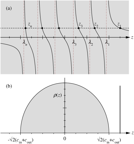
Figure 1: (a) The solid curve represents the right-hand side of Eq. (10) while the dashed horizontal line represents the left-hand side. The points at which the two cross, indicated by the dots, are the solutions $z_{i}$ of the equation, which necessarily fall between the eigenvalues $\lambda_{i}$ of the matrix $\mathbf{X}$ (vertical dashed lines). (b) The spectrum of the modularity matrix is the same of that of the random matrix $\mathbf{X}$ (semicircle), except for the highest eigenvalue $z_{1}$, which is separate from the rest of the spectrum above the transition point given in Eq. (14).

The solutions of this equation, which give the eigenvalues $z$ of the modularity matrix, are represented graphically in Fig. 1a. The right-hand side of the equation has poles at $z=\lambda_{i}$ for all $i$ and, as the figure shows, this means that the eigenvalues must satisfy $z_{1}\geq\lambda_{1}\geq z_{2}\geq\lambda_{2}\geq\ldots\geq z_{n}\geq\lambda_{n}$, where both sets of eigenvalues are numbered in order from largest to smallest. These inequalities place bounds on the eigenvalues $z_{2}\ldots z_{n}$ that become tight as $n\to\infty$, meaning that the spectrum of the modularity matrix is asymptotically identical to that of the random matrix $\mathbf{X}$.

The only exception is the highest eigenvalue $z_{1}$, which is bounded below by $\lambda_{1}$ but unbounded above. To calculate this eigenvalue we note that since $\mathbf{X}$ is a random matrix, its eigenvectors are also random, so that cross-terms cancel in the quantity $(\mathbf{u}^{T}\mathbf{x}_{i})^{2}$ and the average value is simply $|\mathbf{x}_{i}|^{2}/n=1/n$. Taking the average of (10) over the random matrix ensemble in the limit of large $n$ then gives

$${2\over c_{\textrm{in}}-c_{\textrm{out}}} ={1\over n}\left\langle\sum_{i=1}^{n}{1\over z-\lambda_{i}}\right\rangle={1\over n}\left\langle\mathop{\mathrm{missing}}{Tr}(z\mathbf{I}-\mathbf{X})^{-1}\right\rangle$$

$$={z-\sqrt{z^{2}-2(c_{\textrm{in}}+c_{\textrm{out}})}\over c_{\textrm{in}}+c_{\textrm{out}}},$$ (11)

where we have used Eq. (6). Rearranging for $z$, we get our expression for the leading eigenvalue $z_{1}$:

$$z_{1}=\tfrac{1}{2}(c_{\textrm{in}}-c_{\textrm{out}})+{c_{\textrm{in}}+c_{\textrm{out}}\over c_{\textrm{in}}-c_{\textrm{out}}}.$$ (12)

We can use the same method to deduce the spectrum of the full adjacency matrix also. From Eq. (8) we see that the adjacency matrix takes the form $\mathbf{A}=\tfrac{1}{2}(c_{\textrm{in}}+c_{\textrm{out}})\,\mathbf{1}\mathbf{1}^{T}+\mathbf{B}$, which is again a rank-1 matrix plus a random perturbation. By the same argument as before, we can show that this matrix has all eigenvalues the same (to within tight bounds) as those of the modularity matrix, except again for the leading eigenvalue, whose value can be calculated from a relation of the form (10). The end result is that the lower $n-2$ eigenvalues of the adjacency matrix have the same spectrum as the random matrix $\mathbf{X}$ and the top two have the values $z_{1}$, Eq. (12), and

$$z_{2}=\tfrac{1}{2}(c_{\textrm{in}}+c_{\textrm{out}})+1.$$ (13)

With this result, we now have the complete spectrum for both the adjacency matrix and the modularity matrix.

Let us focus on the modularity matrix. The spectrum is depicted in Fig. 1b and consists of the continuous semicirclar band of eigenvalues, Eq. (7), plus the single eigenvalue $z_{1}$, Eq. (12). If the network contained no community structure, then $z_{1}$ would not be separated from the continuous band as it is here. So long as it is well separated the spectrum shows clear evidence of the existence of community structure and one can reasonably say that a calculation of the spectrum constitutes positive “detection” of that structure. Moreover, the signs of the elements of the leading eigenvector provide a good guide to the community division of the network, and indeed this particular method for community identification can be derived directly as a spectral version of the standard method of modularity maximization Newman06b . If, however, the position of the leading eigenvalue passes the edge of the continuous band, the spectrum no longer shows evidence of community structure and spectral algorithms based on the corresponding eigenvector will fail. One might imagine that this point would arrive when $c_{\textrm{in}}=c_{\textrm{out}}$, which is the point at which the network contains no community structure at all, but this is not the case. From Eq. (7) we see that the end of the continuous band falls at $z=\sqrt{2(c_{\textrm{in}}+c_{\textrm{out}})}$ and, setting $z_{1}$ from Eq. (12) equal to this value, we find that we lose the ability to detect community structure at an earlier point, when

$$c_{\textrm{in}}-c_{\textrm{out}}=\sqrt{2(c_{\textrm{in}}+c_{\textrm{out}})}.$$ (14)

This value sets a detectability threshold beyond which the communities are present but cannot be detected. For $c_{\textrm{in}}-c_{\textrm{out}}$ smaller than this value, but greater than zero, community structure is present in the network in the sense that the average probability of edges within groups is measurably higher than that between groups, but we nonetheless fail to find the communities using our spectral method. One can generalize the calculation to networks with a larger number $q$ of communities and we find that a similar transition happens at the point

$$c_{\textrm{in}}-c_{\textrm{out}}=\sqrt{q[c_{\textrm{in}}+(q-1)c_{\textrm{out}}]}.$$ (15)

The existence of a transition of this kind, though not its precise location, was demonstrated previously using different methods by Reichardt and Leone RL08 and there are also close connections between our calculation and the theory of disordered systems KTJ76 .

One might imagine this transition to be a particular property of the spectral method we have considered. Perhaps a different modularity maximization algorithm, one not based on spectral techniques, or a different type of community detection method altogether, would be able to get past this detectability threshold. This, however, is also not the case.

In recent work, Decelle et al. DKMZ11a have used arguments based on the cavity method of statistical physics to demonstrate the existence of a transition akin to the one above in another community detection method, a Bayesian maximum-likelihood method based on directly fitting the stochastic block model to a network. Moreover, their transition falls at the same position as that of Eq. (15). The importance of this result stems from the fact that if we know the model from which a network is drawn, then fitting directly to that model is provably the optimal way of recovering the parameters of the model used to generate the network—including, in this case, the community structure. Thus, as Decelle et al. have pointed out, their maximum-likelihood method is an optimal method in the sense that no method can detect communities in the regime where their method fails. Unfortunately fitting to the stochastic block model turns out to be a poor method of community detection for real-world networks KN11a ; DKMZ11a , but its optimality in the present case is a useful result nonetheless. It implies, given that the detectability transition falls in the same place as for the spectral modularity method, that the modularity method is also optimal in the same sense: no other method will detect communities in the network when the modularity method does not note .

We can take these calculations further. For instance, we can calculate the expected fraction of vertices classified correctly by the spectral algorithm. We can show that the elements of the leading eigenvector $\mathbf{v}$ of the modularity matrix are equal to $\pm\alpha/\sqrt{n}$ plus Gaussian perturbations with variance $(1-\alpha^{2})/n$, where

$$\alpha^{2}={(c_{\textrm{in}}-c_{\textrm{out}})^{2}-2(c_{\textrm{in}}+c_{\textrm{out}})\over(c_{\textrm{in}}-c_{\textrm{out}})^{2}}.$$ (16)

Then the fraction of elements that retain the correct sign and hence give correct classifications of the corresponding vertices is $\tfrac{1}{2}[1+\mathop{\mathrm{missing}}{erf}\sqrt{\alpha^{2}/2(1-\alpha^{2})}]$, where $\mathop{\mathrm{missing}}{erf}x$ is the Gaussian error function.

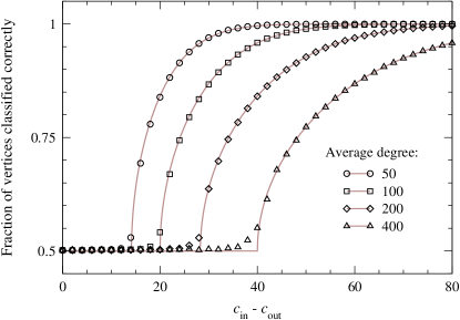
Figure 2: The fraction of vertices correctly classified by the spectral modularity algorithm in networks generated using the block model studied here, as a function of $c_{\textrm{in}}-c_{\textrm{out}}$, for four different values of the average degree as indicated. Points are numerical measurements for networks of $100\,000$ vertices, averaged over 25 networks each; solid curves represent the analytic prediction. The phase transition at which the algorithm fails is clearly visible in each curve.

Figure 2 shows a plot of this quantity as a function of $c_{\textrm{in}}-c_{\textrm{out}}$ for networks with several different values of the average degree, along with results for the same quantity from actual applications of the spectral modularity algorithm to networks generated using the stochastic block model. As the figure shows, the agreement between the two is excellent, except in the immediate vicinity of the phase transition, where finite-size effects produce some rounding of the threshold. The fraction of correctly classified vertices (minus $\frac{1}{2}$) plays the role of an order parameter for the detectability transition. Since it is continuous at the transition point, we have a continuous phase transition.

The calculations presented here could be extended in a number of additional directions. For instance, the results given are accurate for networks with large average degree but for networks with smaller degree there are additional corrections that corresponding to additional terms in the trace, Eq. (5). A calculation of these sub-leading terms would help to complete the picture for low-degree networks. Also our calculations all use the standard stochastic block model, and although this is the model most widely used for benchmark calculations and synthetic tests, other models have been proposed, such as the degree-corrected block model KN11a or more exotic models such as the LFR benchmark networks LFR08 . It would be useful to know if results similar to those described here can be derived for these more complex models.

The authors thank Cris Moore and Lenka Zdeborova for useful comments. This work was funded in part by the National Science Foundation under grants CCF–1116115 and DMS–1107796 and by the Office of Naval Research under grant N00014–11–1–0660.

References

- (1) M. Girvan and M. E. J. Newman, Community structure in social and biological networks. Proc. Natl. Acad. Sci. USA 99, 7821–7826 (2002).
- (2) S. Fortunato, Community detection in graphs. Phys. Rep. 486, 75–174 (2010).
- (3) A. Decelle, F. Krzakala, C. Moore, and L. Zdeborová, Inference and phase transitions in the detection of modules in sparse networks. Phys. Rev. Lett. 107, 065701 (2011).
- (4) A. Condon and R. M. Karp, Algorithms for graph partitioning on the planted partition model. Random Structures and Algorithms 18, 116–140 (2001).
- (5) F. Benaych-Georges and R. R. Nadakuditi, The eigenvalues and eigenvectors of finite, low rank perturbations of large random matrices. Advances in Mathematics 227, 494–521 (2011).
- (6) M. Capitaine, C. Donati-Martin, and D. Féral, The largest eigenvalues of finite rank deformation of large Wigner matrices: Convergence and nonuniversality of the fluctuations. Annals of Probability 37, 1–47 (2009).
- (7) M. E. J. Newman, Modularity and community structure in networks. Proc. Natl. Acad. Sci. USA 103, 8577–8582 (2006).
- (8) J. Reichardt and M. Leone, (Un)detectable cluster structure in sparse networks. Phys. Rev. Lett. 101, 078701 (2008).
- (9) J. M. Kosterlitz, D. J. Thouless, and R. C. Jones, Spherical model of a spin-glass. Phys. Rev. Lett. 36, 1217–1220 (1976).
- (10) B. Karrer and M. E. J. Newman, Stochastic blockmodels and community structure in networks. Phys. Rev. E 83, 016107 (2011).
- (11) Strictly speaking, the results of Ref. DKMZ11a say only that no algorithm will succeed that works in polynomial time—it may be possible, at least in certain parameter regimes, for non-polynomial algorithms to detect the community structure. Non-polynomial algorithms, however, are prohibitively slow for all but the smallest of networks, making communities effectively undetectable past the transition point.
- (12) A. Lancichinetti, S. Fortunato, and F. Radicchi, Benchmark graphs for testing community detection algorithms. Phys. Rev. E 78, 046110 (2008).