90 GHz Continuum Observations of Messier 66

Abstract

Radio emission at around 90 GHz from star-forming galaxies is expected to be strongly dominated by the free-free component due to ionising radiation from massive, short-lived, stars. We present high surface-brightness sensitivity observations at 90 GHz of the nearby star-forming galaxy Messier 66 with resolution of about 9 arcsec (corresponding to a physical scale of about 500 pc) and analyse these observations in combination with archival lower frequency radio and mid-infrared measurements. For the four regions for which the observations support our models we find that the free-free component indeed dominates the emission at 90 GHz, making up 76–90 per cent of the luminosity at this frequency but with the data also consistent with all of the emission being due to free-free. The estimates of free-free luminosities are also consistent, within measurement and decomposition errors, with star-formation rates derived from lower radio frequencies and mid-infrared observations. In our analysis we consider both power-law and curved spectra for the synchrotron component but do not find evidence to support the curved model in preference to the power-law.

1 Introduction

Observations of continuum emission at radio frequencies can provide useful insight into star-formation activity in external galaxies (see, for example, the review by Condon, 1992). This is greatly aided by the fact that radio frequency radiation is unaffected by dust absorption, and by the use of interferometer arrays to give high angular resolution and astrometric accuracy even at long wavelengths.

The continuum emission at these frequencies is due to a combination of two mechanisms that each trace different, but important, stages of evolution of recently formed and short-lived, high-mass stars (Condon, 1992):

1. Free-free radiation (presumably dominant at higher frequencies) which traces the ionising ultraviolet continuum photons from massive young stars whilst they are on the main sequence.

2. Synchrotron radiation, which is dominant at lower radio frequencies and which traces relativistic electrons likely created by supernovae from the same massive stars at the end of their lives.

This utility of radio observations for studying star-formation in external galaxies is already well established at lower frequencies, for example, through large-area, sensitive surveys at frequencies around 1.4 GHz, such as the FIRST (Becker et al., 1995) and NVSS (Condon et al., 1998) surveys. In particular, the observed tight correlation between radio and far-infrared luminosities of local (e.g. Helou et al., 1985) and more distant (e.g. Jarvis et al., 2010) galaxies provides important empirical evidence for use of radio-continuum as a tracer of recent star formation activity.

Observations at higher frequencies ($\nu\gtrsim 10\,\mathrm{GHz}$) are more challenging than at frequencies around 1.4 GHz because the surface brightness of emission from galaxies is fainter while the receiver noise and atmospheric effects are greater. Such observations can, nevertheless, be extremely useful.

High frequency measurements, where total flux density is dominated by free-free emission should enable astronomers to make accurate estimates of both the synchrotron and the free-free components of the emission when combined with data at lower frequencies. The contribution from the free-free component has a a direct physical link to emission in $\mathrm{H}{\alpha}$ and other Hydrogen recombination lines which are some of the most commonly used tracers of star-formation. At the same time though, radio measurements retain the advantage of being unaffected by dust extinction. Hence accurate estimates of free-free emission can be used to calibrate $\mathrm{H}{\alpha}$ other measures of star-formation in dusty environments (see for example Murphy et al., 2011).

Extraction of the flux density of the synchrotron component places constraints on the shape of the synchrotron spectrum. At frequencies above 1 GHz, this shape is determined by the energy distribution of relativistic electrons in the source, which in turn is determined by the energy losses of the electrons accelerated in the supernova remnants. Therefore the shape of the synchrotron spectrum can constrain the evolution of recent star formation activity or cooling processes of the relativistic electrons.

Recently, the combination of large single-dish telescopes and broad-band multi-pixel receivers has significantly improved the achievable surface brightness sensitivity of radio continuum observations at frequencies between 30–100 GHz, while giving angular resolution well matched to characteristic physical length-scales of star-formation in nearby galaxies. We have therefore begun a programme of observations aimed at characterising the free-free emission from nearby galaxies by spatially resolved mapping observations at 90 GHz. Our pilot observations were made at the Green Bank Robert C. Byrd 100-m diameter Telescope (GBT, see Jewell & Prestage, 2004) using the MUSTANG 90 GHz 64-pixel bolometer array with 20 GHz bandwidth (Dicker et al., 2008).

For this initial study it was clear that we needed a comprehensive set of multi-wavelength data so targets were selected from the well observed Spitzer Infrared Nearby Galaxies Survey (SINGS) (Kennicutt et al., 2003) sample. We selected two targets: Messier 66 (M 66, NGC 3627) and Messier 99 (M 99, NGC 4254), which are the two galaxies in the SINGS with highest star-formation rates as given by Kennicutt et al. (2003). Both of these galaxies were observed but did we not reliably detect M 99, hence in this paper show only the results for M 66.

2 Observations and data processing

2.1 GBT/MUSTANG observations

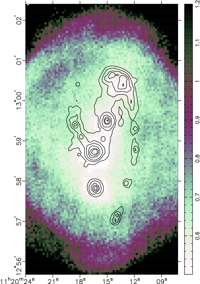
Figure 1: The estimated noise in the final map produced from the GBT/MUSTANG observations shown as colour scale (units are mJy/Beam). Also shown as contours is the 24 $\mu$m Spitzer map of this galaxy which was used to decide where to target the telescope time. The contours are drawn at $(1/2)^{n}\times\textrm{maximum}$.

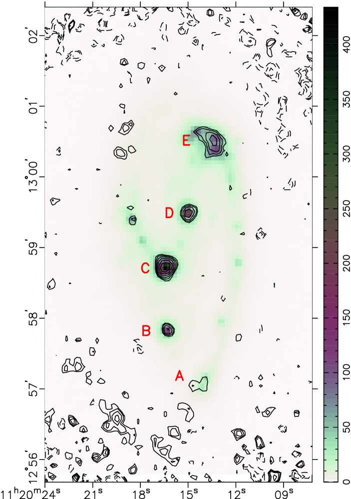
Figure 2: Contours of the results of our GBT+MUSTANG observations overlaid on a Spitzer $24\,\hbox{$\mu$m}$ image. The contours are drawn at intervals of $(3/4)^{n}\times\textrm{maximum}$ and are at 1.02, 0.76, 0.57, 0.43, 0.32, 0.24 and 0.18$\times$ MJy $\mathrm{sr}^{-1}$. The colour scale (representing the $24\,\hbox{$\mu$m}$ emission) is also in units of MJy $\mathrm{sr}^{-1}$. For better presentation the MUSTANG map has been smoothed by a 6 arcsec Gaussian filter before plotting of the contours giving resolution in this diagram of 11.3 arcsec.

Observations with GBT/MUSTANG were made in the winter 2010/2011 observing season under projects GBT09C-020 and GBT10C-011. As the field of view of MUSTANG (about $40\times 40\,$arcsec) is much smaller than the angular extent of M 66 (about $5\times 3$ arcminutes) the observation required the use of a scanning strategy. The choice of the scanning strategy involves a trade-off between area covered and the sensitivity and accuracy of measured fluxes. We decided on a combination of two strategies:

1. A ‘daisy-petal’ strategy which concentrates a large fraction of the integration time in a small angular region. We split the time approximately equally between four centres that were selected based on the Sptizer 24 $\mu$m image of the galaxy;

2. A billiard-ball box scanning strategy which distributes integration approximately uniformly over a rectangular area on the sky. We used box size that was 3 arcminutes on the side and we used three slightly offset centres for the box scanning pattern.

Our total on-source observing time of 5.5 hours was split between these two strategies and all the data from both strategies were analysed together. The resulting noise map is shown in Figure 1 with contours of Sptizer 24 $\mu$m image overlaid on top. It can be seen that although the sensitivity of our observations is best around the prominent knots of 24 micron emission that we were targeting, there is also good sensitivity over a wide, approximately square, area that encompasses the main morphological features of the inner part of this galaxy.

At the beginning at each observing block, and occasionally at other times, the surface of the GBT was adjusted using the Out-Of-Focus (OOF) holography technique (Nikolic et al., 2007) in order to correct for the thermal deformations of the telescope structure. This procedure improves the overall efficiency of observations and also improves the shape of the primary beam of the telescope. During each session the flux calibration standard $\alpha\,$Orianis was observed. Secondary calibrators were also observed, about once per hour, to check the beam shape and enable off-line correction for pointing variation. Our pointing calibrator maps show a beam size of 9.6 arcsec. The observed data were reduced using the suite of IDL-based routines provided by the MUSTANG instrument team. The data reduction strategy and algorithms implemented in this software are described by Mason et al. (2010). We also produced a MUSTANG map smoothed to 15 arcsec resolution for photometry with matched resolution to lower frequency radio data as described below.

2.2 Archival observations

We complement our GBT/MUSTANG observations with archival radio, $\mathrm{H}{\alpha}$ and mid-IR observations. We used the NRAO VLA archive to obtain pre-processed images of M 66 at L, C and X bands (1.4, 4.8 and $8.5\,\mathrm{GHz}$ respectively).

The largest angular scales of emission that the VLA observations are sensitive to are 15–3 arcminutes, which is significantly larger than the largest angular scale that the MUSTANG observations are sensitive to (about 40 arcsec, as discussed below).

At L-band we used data from project AS541, observed by Paladino et al. (2009). Originally this map had a beam of $14.9\times 14.3$ arcsec: this was smoothed to $15.0\times 15.0\,$arcsec (for ease at other frequencies). We use C and X band data from more than one observation. The different maps in each band were first smoothed to $15\times 15$ arcsec resolution before being reprojected (using the CASA task regrid) onto the same basis and then combined via a variance-weighted sum (to give the best off-source noise in the final map).

The final C band map uses data from VLA projects AU078 and AS0551, which had initial resolutions of $\sim 13$ and $\sim 14\,\mathrm{arcsec}$, respectively, prior to smoothing to $15\,\mathrm{arcsec}$. The final X band map uses data from VLA projects AS0551, AU075 and AU078. These had initial resolutions of $\sim\mathrm{9}$, $\sim 7.3$ and $\sim 7.6\,$arcsec respectively, prior to smoothing to $15\,$arcsec.

Our 24 $\mu$m and $\mathrm{H}{\alpha}$ data are derived from the enhanced data products released by the SINGS collaboration (Kennicutt et al., 2003). We used the data released on 10 April 2007 (DR5) as available from IPAC web-site. For estimation of $\mathrm{H}{\alpha}$ luminosities we use the continuum subtracted image which reduces the contamination due to stellar continuum from within M 66 and any faint foreground stars within the measurement apertures (no bright foreground stars are obvious within the apertures). The photometric uncertainty of $\mathrm{H}{\alpha}$ images before continuum subtraction is 10 per-cent so after subtraction the uncertainty is likely to be of order of 20 per-cent. We did not apply a correction for extinction of $\mathrm{H}{\alpha}$ light within the Milky Way (approximately 0.1 magnitude according to maps of Schlegel et al. 1998) as the intrinsic extinction within M 66 is likely to be much higher. We also produced versions of 24 $\mu$m and $\mathrm{H}{\alpha}$ maps smoothed to resolution of 15 arcsec which we used for photometry at resolution which was matched to both radio and MUSTANG data.

3 Analysis and Results

Label	RA	Dec	Radius	Notes
	(J2000)	(J2000)	(arcsec)
A	11:20:14.0	12:57:05.8	12.5	Southern-most part of western spiral arm
B	11:20:16.3	12:57:48.9	13.7	High-recessional velocity, tucked in part of western arm?
C	11:20:16.4	12:58:42.2	16.1	Southern bar end
D	11:20:15.0	12:59:29.0	14.4	Galaxy nucleus
E	11:20:13.7	13:00:30.5	25.9$\times$16.5	Northern bar end

Table 1: Coordinates and sizes of regions used in the analysis of 90 GHz luminosity. The sizes are expressed as radii for regions A–D (which all circular) and as semi-major$\times$ semi-minor axis for region E (which is elliptical with the major axis parallel to the equator).

We analyse the MUSTANG observations quantitatively by identifying regions of significant emissions and extracting fluxes for these regions from maps made at lower radio frequencies and from MUSTANG observations. Because of the data processing required to remove the rapidly varying atmospheric effects, our MUSTANG observations have limited sensitivity to emission on angular scales larger than about 40 arcsec (see the recent work by Mason et al). As a result our selected regions concentrate on knots of emission smaller than 40 arcsec and it is not possible to attempt an analysis of the total flux from this galaxy.

To identify regions of significant emission we smoothed the MUSTANG map to a resolution of 15 arcsec (which is the resolution of our lower-frequency radio data) and identified by eye in this map five regions of well-detected 90 GHz emission. The regions are labelled on Figure 2 and their coordinates and sizes are shown in Table 1. We carried out photometry by simple addition of flux densities in the regions; for ‘A’–‘D’ we used circular apertures with centres and radii as given in Table 1 and for region ‘E’ we used an elliptical aperture with the centre, semi-major and semi-minor axis also given in Table  1 and with the major axis parallel to the equator. All of the regions are signifantly larger than the resolution of the observed maps and in the case of Spitzer they also contain the first diffraction ring of the telescope at 24 $\mu$m. Nevertheless, to reduce the effects of different resolutions, all of the photometry measurements were made on maps smoothed to 15 arcsec resolution, set by our lowest resolution radio-frequency data set.

We did not attempt to calculate and subtract local diffuse background. As described above, MUSTANG data processing regardless filters out most emission on angular scales larger than about 40 arcsec, effectively removing the diffuse emission. Lower frequency radio observations were made with minimum spacing of interferometer elements such that much larger scales are retained. Therefore, at lower frequencies there is some additional uncertainty in flux density measurements due to this diffuse local background. As the source of this local background may be diffusion of relativistic electrons from knots of star-formation, any attempt to remove it may make interpretation of subsequent results much more difficult and so we have chosen not to do so. The 24 $\mu$m and $\mathrm{H}{\alpha}$ are ‘total power’ measurements, i.e., all angular scales larger than the angular resolution are retained, and so these data also have additional uncertainty associated with diffuse local background. Murphy et al. (2011) find better match between estimates of star-formation rates from synchrotron and free-free components when the local background is not removed and also find that background removal does not significantly affect the decomposition of spectra into free-free and synchrotron components.

For the following analysis we adopt a distance to M 66 of 11.1 Mpc derived from Cepheid measurement by Saha et al. (1999), which means that one arcminute corresponds to approximately $3.2\,\mathrm{kpc}$ projected distance.

Label	$F_{\nu}(1.4\,\mathrm{GHz})$	$F_{\nu}(4.9\,\mathrm{GHz})$	$F_{\nu}(8.5\,\mathrm{GHz})$	$F_{\nu}(90\,\mathrm{GHz})$	$F_{\nu}(24\,\hbox{$\mu$m})$
	(mJy)	(mJy)	(mJy)	(mJy)	(mJy)
A	$1.9\pm 0.1$	$1.5\pm 0.1$	$0.9\pm 0.05$	$1.6\pm 0.4$	110
B	$9.1\pm 0.5$	$4.6\pm 0.2$	$2.8\pm 0.1$	$1.7\pm 0.3$	310
C	$39.6\pm 2.0$	$18.3\pm 1$	$12.0\pm 0.6$	$7.4\pm 1.1$	1160
D	$24.1\pm 1.0$	$10.6\pm 0.6$	$6.0\pm 0.3$	$2.7\pm 0.4$	490
E	$47.6\pm 2.0$	$22.6\pm 1.1$	$14.4\pm 0.7$	$7.4\pm 1.1$	1190

Table 2: Measured fluxes densities of regions as describe in Table 1.

Region	$\left<\nu_{\rm SN}\right>$	$\left<\alpha\right>$	$\left<\Psi\right>$	$\Psi_{\mathrm{H}{\alpha}}$	$\Psi_{24\,\hbox{$\mu$m}}$	$f_{{\rm th},90\,\mathrm{GHz}}$	$f_{{\rm th},33\,\mathrm{GHz}}$
	($10^{-3}\mathrm{yr}^{-1}$)		($\mathrm{\textrm{M}_{\odot}}\,\mathrm{yr}^{-1}$)	($\mathrm{\textrm{M}_{\odot}}\,\mathrm{yr}^{-1}$)	($\mathrm{\textrm{M}_{\odot}}\,\mathrm{yr}^{-1}$)
A			$0.20\pm 0.07^{*}$	0.024	0.07
B	$1.2\pm 0.09$	$-0.90\pm 0.13$	$0.13\pm 0.04$	0.029	0.17	$0.83\pm 0.13$	$0.72\pm 0.13$
C	$5.0\pm 0.4$	$-1.02\pm 0.16$	$0.64\pm 0.14$	0.088	0.51	$0.90\pm 0.09$	$0.82\pm 0.09$
D	$3.4\pm 0.2$	$-0.93\pm 0.10$	$0.20\pm 0.07$	0.053	0.25	$0.76\pm 0.17$	$0.61\pm 0.17$
E	$6.2\pm 0.5$	$-0.90\pm 0.13$	$0.58\pm 0.19$	0.164	0.52	$0.80\pm 0.20$	$0.68\pm 0.20$

Table 3: Derived properties of regions listed in Table 1. Column $\nu_{\rm SN}$ is the supernova rate, $\alpha$ is the index of the power-law synchrotron component, $\Psi$ is the star-formation rate derived from the free-free component, $\Psi_{\mathrm{H}{\alpha}}$ is the star-formation rate derived from $\mathrm{H}{\alpha}$ emission and $\Psi_{24\,\hbox{$\mu$m}}$ is the star-formation rate derived from 24 $\mu$m mid-infrared emission. Columns $f_{{\rm th},90\,\mathrm{GHz}}$ and $f_{{\rm th},33\,\mathrm{GHz}}$ are the predicted fractions of total flux density that are due to free-free emission at 90 and 33 GHz respectively and are computed by marginalisation of the model over the full joint posterior distribution. ^∗Since the model fit for region ‘A’ is poor, this SFR was derived by direct application of Equation 2.

Figure 3: Observed flux densities of the five regions with detections at 90 GHz (right-most points) and at other frequencies with matched resolution we consider in this letter.

3.1 Models

We consider two models for the radio spectra. The first model consists of a simple power-law synchrotron component (calibrated using relations in Condon, 1992) and a free-free component that was also modelled as a power law and was calibrated following Murphy et al. (2011). The second model includes the possibility of a curvature or break in the synchrotron component by modelling it as a parabola in log-log space as done by Williams & Bower (2010).

The synchrotron component can therefore be represented in both models by:

$$L_{\nu,\rm SN} =\frac{\nu_{\rm SN}}{1\,\mathrm{yr}^{-1}}1.3\times 10^{23}\,\mathrm{W}\,\mathrm{Hz}^{-1}\,\exp\left(\alpha\xi+\gamma\xi^{2}\right),$$ (1)

where:

$\xi$

is a dimensionless frequency parameter $\xi=\log\left(\frac{\nu}{1\,\mathrm{GHz}}\right)$;

$\nu_{\rm SN}$

is the rate of supernova explosions;

$\alpha$

is the linear slope of the synchrotron spectrum (i.e. the spectral index, if the synchrotron spectrum is not curved);

$\gamma$

is a parametrisation of the curvature of the synchrotron spectrum, and is fixed at zero for the simple power-law model.

The free-free component is given by:

$$L_{\nu,\rm FF}=2.17\times 10^{20}\,\mathrm{W}\,\mathrm{Hz}^{-1}\,\frac{\Psi}{1\,\mathrm{\textrm{M}_{\odot}}\,\mathrm{yr}^{-1}}\left(\frac{\nu}{1\,\mathrm{GHz}}\right)^{-0.1}$$ (2)

where $\Psi$ is the star-formation rate. This is an update by Murphy et al. (2011) of the Condon (1992) relationship using the initial mass function as described by Kroupa (2001) and extending the lower limit of the mass function to $0.1\,\textrm{M}_{\odot}$.

3.2 Analysis

We performed Bayesian statistical inference (see for example Jaynes, 2003; von Toussaint, 2011) of the observed flux densities for each region and these two models using the radiospec package described by Nikolic (2009). As parameters $\nu_{\rm SN}$ and $\Psi$ can be considered scale parameters we adopt log-flat, non-informative, priors for them. For parameter $\alpha$ we adopted a flat prior $-1.5<\alpha<-0.5$ and for parameter $\gamma$ a flat prior $-1<\gamma<0$.

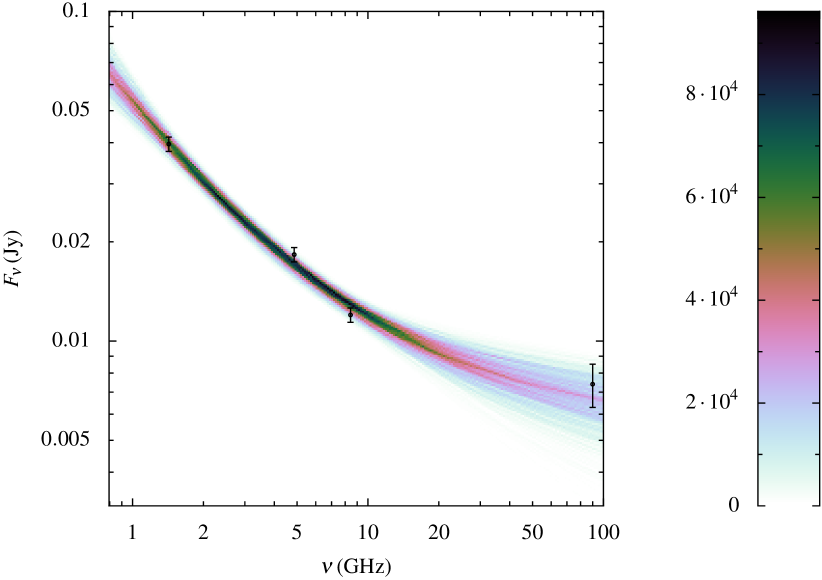
Figure 4: Fan-diagram plot of the fit of power-law synchrotron and free-free model for observed radio emission from region ‘C’. The points and error bars are the measured flux densities for this region. The colour scale represents the relative probability distribution of possible spectra given the power-law synchrotron and free-free components model and the inferred posterior distribution of parameters. The overall magnitude of the colour scale is set by requirement that the integral along each vertical slice of the distribution equals the Bayesian evidence (marginal likelihood) for this model.

The computed Bayesian evidence (also known as marginal likelihood) did not show preference for the curved synchrotron component model in any region. If we nevertheless adopt the curved synchrotron model we can place a limit on the curvature parameter of $\gamma>-0.4$ for all of the regions. The analysis would be better able to discriminate between these models if more frequency data points were available, including at frequencies below 1.4 and around 5 GHz; and, naturally, if the measurement uncertainties (which are dominated by calibration uncertainties) were reduced. For the remainder of analysis we concentrate on the simpler power-law synchrotron model.

The Bayesian evidence also showed that the quality of the fit to measured flux densities of region ‘A’ was poor and therefore we have not used the Bayesian inference to derive physical properties of this region. Given the inconsistent flux densities at lower radio frequencies and that region ‘A’ is in a part of our GBT/MUSTANG map with higher noise, the flux density measurement for region ‘A’ should be interpreted with caution.

As an illustration of the inference process, we show in Figure 4 the fan-diagram (see Nikolic, 2009) of the fit of this model to the brightest region which is region ‘C’.

The Bayesian analysis results in a joint posterior probability distribution of all parameters. We have summarised the marginalised probability distributions of each parameter in Table 3 by its mean and standard deviation, together with simple estimates of star-formation rates from 24 $\mu$m and $\mathrm{H}{\alpha}$ emission (made using relations given by Murphy et al., 2011). Such a summary does not however give a complete picture of the posterior distribution when it is not normally distributed or when there are significant correlations between parameters.

This correlation is most significant in our analysis for parameters $\Psi$ and $\alpha$ as illustrated in Figure 5 for the case of region ‘C’ (regions ‘B’–‘E’ show similar results). The top panel of this figure shows the marginalised posterior probability of $\Psi$ and it can be noted that although it has a well defined peak it also shows a tail of low values. The reason for this tail of low values is explained in the lower panel of this figure which shows there is a degeneracy (but at a relatively low probability) between parameters $\Psi$ and $\alpha$. Therefore even with measurements at $90\,\mathrm{GHz}$, the uncertainty in $\alpha$ still contributes to an extent to the accuracy with which can $\Psi$ be inferred.

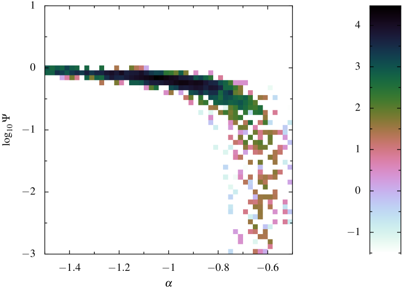
Figure 5: Marginal posterior distribution of the $\Psi$ parameter (star-formation rate from free-free luminosity, upper panel) and joint posterior probability distribution of parameters $\Psi$ and $\alpha$ (slope of the synchrotron power law, lower panel) from the analysis of region ‘C’. The colour scale in the lower panel represents $\log_{10}$ of the posterior probability which is normalised so that its integral over the area of the plot is equal to the Bayesian evidence.

3.3 Discussion

It is clear from Figure 2 that the morphology of free-free and mid-infrared emission are similar. Quantitatively, the star-formation rates estimated from free-free emission, $\Psi$, are in broad agreement with the estimates from 24 $\mu$m emission for regions ‘B’–’E’, i.e., they are all within one standard deviation of the posterior of each other. It appears therefore that at these modest star-formation rates and at physical resolutions of about 1 kpc there is no deficit in free-free emission like found in luminous and ultra-luminous infra-red starburst galaxies by Clemens et al. (2010) and Leroy et al. (2011) but that instead the measured emission is consistent with existing models, as also found for nearby galaxies by Peel et al. (2011) and Murphy et al. (2011). Also shown in Table 3 are star-formation rates estimated from $\mathrm{H}{\alpha}$ measurements. These are much (by a factor of 3 to 6) smaller than the rates derived from 90 GHz and 24 $\mu$m observations and the primary cause of this is likely to be internal extinction of the $\mathrm{H}{\alpha}$ radiation within M 66.

Additionally, the inferred supernova rates $\nu_{\rm SN}$ can also be compared to the estimates of star-formation rates by multiplying them by a factor of 86.3 (Murphy et al., 2011). We find that for regions ‘B’, ’C’ and ’E’ the star-formation rate inferred in this way underestimates the free-free estimates by an average of 21 per-cent but this result is statistically weak because the errors for each region are large and because the errors are likely to be correlated between the regions, i.e. , they are dominated by systematic calibration uncertainty which is likely to affect each of the regions in a similar way. This discrepancy is significantly smaller than the average factor of 2 found by Murphy et al. (2011) for the case when they (like we) do not subtract the local background. This difference may be due to the high inclination of M 66 which means that diffusion of electrons within the disc reduces the surface brightness by a smaller factor compared to a face-on galaxy, or because the burst of star formation in M 66 is more recent leaving little time for diffusion of relativistic electrons.

We did not consider region ‘D’ in this discussion as it is coincident with the nucleus of M 66 which is classified as transition/Seyfert 2 nucleus by Ho et al. (1997) and so there is the additional uncertainty of a possible contribution to synchrotron and mid-infrared emission from the active galactic nucleus.

From the models we also compute and show in Table 3 the fraction of predicted flux density at 90 GHz and 33 GHz that is due to free-free emission (the “thermal fraction”). We find that the mean thermal fraction at 90 GHz is about 83 per cent but is also consistent (due to large estimated error) with essentially all of the emission being due to the free-free component. At 33 GHz we predict a thermal fraction of around 71 per cent which is consistent with the 79 per cent that Murphy et al. (2011) find when local diffuse background is not subtracted.

The detection of region ‘A’ at 90 GHz is at the level of four standard errors so it is somewhat statistically uncertain. If the true flux density of this region is indeed close to our measured value then the spectrum is rising between 8.5 and 90 GHz which is not possible in the models we used in the analysis and consequently the Bayesian evidence of both of our models for this region is very poor. For this reason we do not show the results of Bayesian analysis for this region. A possible explanation of such a rising spectrum would be a very compact, high density H ii region which should be easy to test using high spatial resolution observations at 90 GHz using an interferometer.

Finally, we briefly discuss advantages and efficiency of bolometer observations at 90 GHz of nearby galaxies such as those presented in this paper. Our results above show that close to all of the flux density at 90 GHz is due to free-free emission and this is one of the primary advantages of such observations, as free-free emission is closely related to the number of ionising photons emitted by young stars yet unaffected by dust obscuration. Hence observations at 90 GHz can be used to estimate the rate of ionising photon absorption by hydrogen atoms without uncertainties associated with correction for dust extinction of $\mathrm{H}{\alpha}$ measurements. This is essentially what the $\left<\Psi\right>$ column in Table 3 measures (after conversion to star-formation rate) and it can be noted that our estimated uncertainty is still 20–30 per cent. This is due to the relatively large uncertainty we assume for our absolute calibration of our observations at 90 GHz (15 per cent) and uncertainty in removal of the small but not well known synchrotron component at this frequency. Experience with bolometer observations at 90 GHz and improvements in processing algorithms should reduce the absolute calibration uncertainty in the future while further studies at intermediate frequencies should help us better constrain and understand the synchrotron component in star-forming galaxies at these frequencies.

Star-formation which can be measured with observations like ours can be approximately estimated by combining Equation 2 and the noise in our maps which is approximately 0.5 mJy/beam in the best parts. This leads to estimate of $1\sigma$ sensitivity to unresolved star formation of about $(D/10\,\mathrm{Mpc})^{2}0.05\,\mathrm{\textrm{M}_{\odot}}\,\mathrm{yr}^{-1}$, where $D$ is the distance to the galaxy, while for resolved star formation it is about $0.22\,\mathrm{\textrm{M}_{\odot}}\,\mathrm{yr}^{-1}\,\mathrm{kpc}^{-2}$. Our non-detection of Messier 99 is consistent with these sensitives when we use the Spitzer 24 $\mu$m map of this galaxy to predict star formation distribution. Adopting a distance of 20 Mpc, such an estimate leads to star-formation rate of $0.36\,\mathrm{\textrm{M}_{\odot}}\,\mathrm{yr}^{-1}$ in the compact central region of this galaxy which is below the $2\sigma$ level expected at this distance.

4 Conclusions

We present results of a pilot project to observe nearby galaxies with GBT/MUSTANG to high surface brightness sensitivity. We find:

1. GBT/MUSTANG can measure the continuum emission at 90 GHz from nearby star-forming galaxies with resolution around 9 arcsec and in our case $1\sigma$ sensitivity to unresolved sources that corresponds to a star-formation rate of approximately $(D/10\,\mathrm{Mpc})^{2}0.05\,\mathrm{\textrm{M}_{\odot}}\,\mathrm{yr}^{-1}$;

2. These measurements in turn constrain the free-free emission associated with ionising radiation from young stars ;

3. For the case of M 66, the measured free-free emission is consistent, to within one standard deviation, with star-formation rate estimates from 24 $\mu$m Spitzer observations; the free-free derived star-formation rates are higher by an average of 21 per cent than the rates derived from low frequency radio data but this is a statistically weak discrepancy;

4. Analysis of measurements at L, C, X-band and 90 GHz do not prefer a curved synchrotron specturm as opposed to a simple power law synchrotron and free-free components model;

5. The estimate of the thermal fraction at 90 GHz is close to unity; at 33 GHz it is estimated to be around 71 per cent.

References

- Becker et al. (1995) Becker R. H., White R. L., Helfand D. J., 1995, ApJ, 450, 559
- Clemens et al. (2010) Clemens M. S., Scaife A., Vega O., Bressan A., 2010, MNRAS, 405, 887. \hrefhttp://arxiv.org/abs/1002.3334 \patharXiv:1002.3334
- Condon (1992) Condon J. J., 1992, ARA&A, 30, 575
- Condon et al. (1998) Condon J. J., Cotton W. D., Greisen E. W., Yin Q. F., Perley R. A., Taylor G. B., Broderick J. J., 1998, AJ, 115, 1693
- Dicker et al. (2008) Dicker S. R., et al., 2008, in Society of Photo-Optical Instrumentation Engineers (SPIE) Conference Series, Vol. 7020, Society of Photo-Optical Instrumentation Engineers (SPIE) Conference Series. \hrefhttp://arxiv.org/abs/0907.1306 \patharXiv:0907.1306
- Helou et al. (1985) Helou G., Soifer B. T., Rowan-Robinson M., 1985, ApJ, 298, L7
- Ho et al. (1997) Ho L. C., Filippenko A. V., Sargent W. L. W., 1997, ApJS, 112, 315. \hrefhttp://arxiv.org/abs/arXiv:astro-ph/9704107 \patharXiv:arXiv:astro-ph/9704107
- Jarvis et al. (2010) Jarvis M. J., et al., 2010, MNRAS, 409, 92. \hrefhttp://arxiv.org/abs/1009.5390 \patharXiv:1009.5390
- Jaynes (2003) Jaynes E. T., 2003, Probability Theory : The Logic of Science. Cambridge University Press
- Jewell & Prestage (2004) Jewell P. R., Prestage R. M., 2004, in Society of Photo-Optical Instrumentation Engineers (SPIE) Conference Series, Vol. 5489, Society of Photo-Optical Instrumentation Engineers (SPIE) Conference Series, J. M. Oschmann Jr., ed., pp. 312–323
- Kennicutt et al. (2003) Kennicutt Jr. R. C., et al., 2003, PASP, 115, 928. \hrefhttp://arxiv.org/abs/astro-ph/0305437 \patharXiv:astro-ph/0305437
- Kroupa (2001) Kroupa P., 2001, MNRAS, 322, 231. \hrefhttp://arxiv.org/abs/arXiv:astro-ph/0009005 \patharXiv:arXiv:astro-ph/0009005
- Leroy et al. (2011) Leroy A. K., et al., 2011, ApJ, 739, L25. \hrefhttp://arxiv.org/abs/1107.4109 \patharXiv:1107.4109
- Mason et al. (2010) Mason B. S., et al., 2010, ApJ, 716, 739
- Murphy et al. (2011) Murphy E. J., et al., 2011, ApJ, 737, 67. \hrefhttp://arxiv.org/abs/1105.4877 \patharXiv:1105.4877
- Nikolic (2009) Nikolic B., 2009, ArXiv e-prints, 0912.2317. \hrefhttp://arxiv.org/abs/0912.2317 \patharXiv:0912.2317
- Nikolic et al. (2007) Nikolic B., Prestage R. M., Balser D. S., Chandler C. J., Hills R. E., 2007, A&A, 465, 685. \hrefhttp://arxiv.org/abs/arXiv:astro-ph/0612249 \patharXiv:arXiv:astro-ph/0612249
- Paladino et al. (2009) Paladino R., Murgia M., Orrù E., 2009, A&A, 503, 747. \hrefhttp://arxiv.org/abs/0905.3643 \patharXiv:0905.3643
- Peel et al. (2011) Peel M. W., Dickinson C., Davies R. D., Clements D. L., Beswick R. J., 2011, MNRAS, 416, L99. \hrefhttp://arxiv.org/abs/1105.6336 \patharXiv:1105.6336
- Saha et al. (1999) Saha A., Sandage A., Tammann G. A., Labhardt L., Macchetto F. D., Panagia N., 1999, ApJ, 522, 802. \hrefhttp://arxiv.org/abs/arXiv:astro-ph/9904389 \patharXiv:arXiv:astro-ph/9904389
- Schlegel et al. (1998) Schlegel D. J., Finkbeiner D. P., Davis M., 1998, ApJ, 500, 525. \hrefhttp://arxiv.org/abs/arXiv:astro-ph/9710327 \patharXiv:arXiv:astro-ph/9710327
- von Toussaint (2011) von Toussaint U., 2011, Rev. Mod. Phys., 83, 943. Available from: \urlhttp://link.aps.org/doi/10.1103/RevModPhys.83.943
- Williams & Bower (2010) Williams P. K. G., Bower G. C., 2010, ApJ, 710, 1462. \hrefhttp://arxiv.org/abs/0912.0014 \patharXiv:0912.0014