On the unconstrained expansion of a spherical plasma cloud turning collisionless : case of a cloud generated by a nanometer dust grain impact on an uncharged target in space.

Abstract

Nano and micro meter sized dust particles travelling through the heliosphere at several hundreds of km/s have been repeatedly detected by interplanetary spacecraft. When such fast moving dust particles hit a solid target in space, an expanding plasma cloud is formed through the vaporisation and ionisation of the dust particles itself and part of the target material at and near the impact point. Immediately after the impact the small and dense cloud is dominated by collisions and the expansion can be described by fluid equations. However, once the cloud has reached $\mu{\rm m}$ dimensions, the plasma may turn collisionless and a kinetic description is required to describe the subsequent expansion. In this paper we explore the late and possibly collisionless spherically symmetric unconstrained expansion of a single ionized ion-electron plasma using N-body simulations. Given the strong uncertainties concerning the early hydrodynamic expansion, we assume that at the time of the transition to the collisionless regime the cloud density and temperature are spatially uniform. We do also neglect the role of the ambient plasma. This is a reasonable assumption as long as the cloud density is substantially higher than the ambient plasma density. In the case of clouds generated by fast interplanetary dust grains hitting a solid target some $10^{7}$ electrons and ions are liberated and the in vacuum approximation is acceptable up to meter order cloud dimensions. As such a cloud can be estimated to become collisionless when its radius has reached $\mu$m order dimensions, both the collisionless approximation and the in vacuum approximation are expected to hold during a long lasting phase as the cloud grows by a factor $10^{6}$. With these assumptions, we find that the transition from the collisional to the collisionless regime could occur when the electron Debye length $\lambda_{\rm D}$ within the cloud is much smaller than the cloud radius $R_{0}$, i.e. $\Lambda\equiv\lambda_{\rm D}/R_{0}\ll 1$. This implies a quasi-neutral expansion regime where the radial electron and ion density profiles are equal through most of the cloud except at the cloud-vacuum interface. The consequence of $\Lambda$ being much smaller that unity implies that the electrostatic fields within a cloud generated by a dust impact on a neutral target is $\sim 100$ times weaker than in the case of grains hitting a spacecraft, where the positive potential of the target is strong enough to strip-off all the electrons from the expanding cloud leading to a "Coulomb explosion" like regime (e.g. Peano et al (2007) [1]).

1 Introduction

The problem of the expansion of a plasma into vacuum has received much attention in recent years mainly in the context of the understanding of the expansion of plasma clouds generated by laser irradiated materials [2, 3, 4, 5, 6]. The expansion of negatively charged dust particles in cometary tails [7, 8] and the expansion of the solar wind plasma into the wake region of inert objects such as asteroids or the moon [9] has also stimulated theoretical and numerical studies on the problem of the expansion of a plasma into vacuum. The impact of fast moving clusters of atoms or molecules on a solid surface are also known to produce expanding plasma clouds. In particular, dust particles, typically in the micro to nano meter range, hitting spacecraft at velocities up to hundreds of km/s have been repeatedly detected in space [10, 11, 12, 13, 14, 15, 16, 17, 18]. In most laser plasmas experiments only the electrons (not the ions) are heated by the laser’s electromagnetic field. In these experiments, the initial state of the plasma is characterised by of hot electron population, carrying all of the energy, and a cold ion population, too tenuous for collisions to operate. On the other hand, dust impact generated plasma clouds are initially dense enough for electrons and ions to be in thermodynamic equilibrium everywhere within the cloud with the possible exception of the cloud/vacuum interface. One fluid models [19, 20, 21, 22], or two fluid models allowing for a separate description of ions and electrons (see the classical review paper [23]) are the appropriate tools to model the collisional regime of the expansion. At some point however, provided the expansion takes place in vacuum or in a tenuous plasma and provided the collisional mean free path of an electron grows faster than the cloud radius $R$, the expansion becomes collisionless and a kinetic description necessary. Typically a nano meter dust particle impact at the solar wind speed is expected to ignite an expanding plasma cloud with some $10^{7}$ electrons and ions and a characteristic temperature of 10eV turns collisionless at cloud dimensions $R\gtrsim\mu{\rm m}$. The cloud then continues its expansion in the free collisionless regime until its density has declined to a value comparable to the ambient plasma density, which at Earth’s orbit occurs for a meter order cloud radius. Thus, during the free collisionless expansion regime the cloud radius grows by a factor of order $10^{6}$ before it merges with the ambient plasma. At such small scales magnetic forces can be safely neglected given that the Larmor radius of a low energy 1eV electron in interplanetary space already exceeds 600 m.

The aim of this paper is to explore the unconstrained collisionless expansion of a plasma cloud using kinetic simulations. The plasma made of identical single ionised ions and an equal number of electrons is assumed to be initially confined within a spherical shell which will be instantly removed to let the plasma expand freely into vacuum. The plasma is assumed to be initially at rest and at thermodynamic equilibrium implying equal ion and electron temperatures. This kind of initial condition differs from most of the published papers on the expansion of a plasma into vacuum where ions are generally assumed to be cold as in most laser heated laboratory plasma (e.g. [24, 25, 26, 27] using fluid models, or [28, 1] using kinetic models). We note that some of the presented results, in particular concerning the shape of the asymptotic electron velocity distribution function (see Figure 5), have been anticipated by Manfredi and Mola (1993) [29] using the strictly collisionless Vlasov model and a hotter plasma. In this work we use a one dimensional N-body scheme to solve the equations of motion for a large number of ions and electrons so that collisions are not exclude a priori. The similarities between our results and the results by Manfredi and Mola are then due to the fact that we assume the cloud to be marginally collisional from the beginning with the expansion further reducing the collisionality until an asymptotic “frozen” self-similar state is reached. It is worth noting that analytic self-similar solutions in the quasi-neutral limit, where charge separation is assumed to be small exist in the literature (see e.g. [26, 30]). Such solutions are expected to hold in the limit of an electron Debye length being small with respect to the cloud dimension which we do suggest to be the case if the latter turns collisionless during its expansion. However, the formation of an extended electron precursor, which appears to be inevitable in the spherical case [25, 27], suggest that the quasi-neutral assumption necessarily fails in the electron dominated, outer shells of the cloud.

The plan of the paper is as follows. In Section 2 we introduce the basic parameters and equations relevant to the problem of the expansion of a spherically symmetric plasma. Since we focus our attention to the case of clouds which are initially collision dominated, we complete Section 2 with an outline the necessary conditions for a transition towards a collisionless regime to occur. In section 3 the initial conditions and parameters for a simulation of a typical case are specified. The results of the simulation are discussed in detail in sections 4 to 7. A summary of the paper is presented in section 9.

2 Definition of the problem

We consider a spherically symmetric electron-ion plasma cloud made of $N/2$ singly charged ions and $N/2$ electrons expanding into vacuum. During the first phase of the expansion the plasma is supposed to be sufficiently dense to be dominated by interparticle collisions. This phase is conveniently described by fluid dynamics [19, 21, 22, 23] and will not be treated in this paper. Under favourable conditions, however, the cloud radius $R(t)$ may grow larger than the collisional mean free path of a thermal electron. At this particular radius $R=R_{0}$ the cloud plasma becomes collisionless and enters a new regime which is no longer tractable within the frame of a fluid theory. The reason for using electrons instead of ions to define the end of the collisional regime is that for a given temperature the collisionality of the latter may be substantially reduced as soon as the external shells of the cloud start moving faster than the ion thermal velocity as under such circumstances ions can no longer approach each other. As we shall see below the expansion velocity is indeed suprathermal for the ions after a short lapse of time roughly corresponding to the time required for the cloud to double its radius.

2.1 Initial state of the cloud

As the expansion is supposed to be collisional for $R<R_{0}$ we assume that electrons and ions are initially (at time $t_{0}$) in the state of thermodynamic equilibrium and confined within the spherical shell $R=R_{0}$. As the state of the plasma at the end of the fluid (collision dominated) phase is generally not known as it strongly depends on the cloud structure at the time of its formation and also on the adopted equation of state, we assume that ions and electrons are initially distributed according to a zero mean velocity Maxwell-Boltzmann distribution with temperature $T_{0}$. In order for the electron mean free path to be uniquely defined we do also assume that at $t=0$ the density within the cloud is spatially uniform. A more realistic description of the initial state of the cloud when $R=R_{0}$, not even taking into account the presence of different ion species and neutrals (e.g. [31]), should include a non zero, radially varying fluid velocity profile, and a complex plasma-vacuum interface (see [23]). We note that even if one assumes that the early, collisional phase is governed by simple inviscid gas dynamics, the spatial and temporal structure of the expanding cloud has been shown to strongly depend on both the assumed energy equation (isentropic, isothermal, …) and on the density and temperature distribution within the cloud at the time of its formation [21, 19, 22]. A few words on the radial velocity profile $u(r,t)$. In situations where the cloud radius $R$ is allowed to grow much larger than the radius of the cloud at the time of its formation the evolution must be close to self-similar. Unlike the density and temperature profiles, the velocity profile then converges towards $u=r/t$ for $t\rightarrow\infty$ independently of the conditions at the time of formation and independently of whether the governing equations are fluid [21, 19, 22, 32] or kinetic [1, 25, 27]. One may then be tempted to select a linear velocity profile $u(r,t=0)=r/\delta t$ as initial condition for the collisionless regime, where $-\delta t$ is the instant of cloud formation. Unfortunately, such a profile is a priori incompatible with the assumption of a constant density profile unless very special, and unlikely, conditions exist at $t=-\delta t$. More sophisticated initial conditions based on approximate self-similar solutions from compressible gas dynamics (e.g. [19, 22]) will be discussed in a future publication.

2.2 Basic parameters

Previous works [25, 1, 27] on the spherical expansion of a plasma into vacuum have pointed out that the problem is characterized by the dimensionless parameter $\Lambda\equiv\lambda_{\rm D}/R_{0}$ at $t=0$, where $\lambda_{\rm D}$ is the electron Debye length (SI units)

$$\lambda_{\rm D}=\left(\frac{\varepsilon_{0}T}{ne^{2}}\right)^{1/2}.$$ (1)

In equation (1) $e$ is the absolute value of the electron charge, $\varepsilon_{0}$ the permittivity of free space, $T$ the temperature and $n$ the electron density. In equation (1) and during the remaining of this paper we assume that temperatures are given in energy units, i.e. temperatures are implicitly multiplied by the Boltzmann constant $k_{\rm B}$. In situations when $\Lambda\ll 1$ the thermal energy of the electrons is too low to allow for a substantial charge separation at the cloud surface: the expansion is quasi-neutral. On the other hand, in situations when $\Lambda\gg 1$ most of the electrons are energetic enough to overcome the electrostatic forces which bind them to the ions. In this case, the cloud becomes positively charged on a time scale of the order of $R_{0}/v_{\rm e}$ ($v_{\rm e}\equiv(2T/m_{\rm e})^{1/2}$ is the electron thermal velocity) and the associated peak electric field is much stronger than in the quasi-neutral case. In the limit $\Lambda\rightarrow\infty$ (the so called Coulomb explosion) all electrons escape from the cloud and the expansion is driven mainly by the repulsive forces pushing the unshielded ions away from each other.

Let us now estimate the parameter $\Lambda$ at time $t=0$, when the plasma becomes collisionless. To this end we use the Fokker-Planck expression for the mean free path of a thermal electron

$$l_{\rm e}=16\pi\varepsilon_{0}^{2}\>\frac{T^{2}}{e^{4}n\lambda}$$ (2)

where $\lambda\equiv\ln(\lambda_{\rm D}/r_{\rm s})$ is the Coulomb logarithm and $r_{\rm s}$ the strong interaction radius, usually defined as the larger of the classical distance for a strong electrostatic interaction between thermal electrons $e^{2}/(12\pi\varepsilon_{0}T)$ or the de Broglie length for a thermal electron $\hbar/(3m_{\rm e}T)^{1/2}$, where $\hbar$ is the reduced Planck constant. For temperatures exceeding 9eV the quantum mechanical definition should therefore be used to define the $r_{\rm s}$. As typical cloud temperatures are expected to be of the order of a few eV up to at most 20eV and also because of the classical nature of the presented simulation, we stick to the classical definition throughout the paper. We emphasise that this assumption does not invalidate the subsequent discussions and the presented simulation for the case of temperatures higher than 9eV since we do only require $r_{\rm s}$ being small with respect to the radius of the spherical shell $r_{\rm min}$ defining the inner boundary of the simulation domain (see 3). Now, even for an exceedingly hot cloud at 81eV, the quantum mechanical definition of $r_{\rm s}$ is just three times larger than the classical definition.

Equation (2) is a good estimate of the mean free path of a thermal electron in a weakly coupled plasma with $\lambda\gtrsim 10$. For values $2\lesssim\lambda\lesssim 10$ equation (2) may still be used as a fair estimate of $l_{\rm e}$. By noting that the initial density $n_{0}$ is related to the cloud radius and the total number of electrons $N/2$ via

$$n_{0}=\frac{N/2}{\displaystyle\frac{4\pi}{3}R_{0}^{3}}$$ (3)

it follows from (1) and by setting $l_{\rm e}(t=0)=R_{0}$ in (2) that the dimensionless parameter $\Lambda$ only depends on the total number of charged particles $N$ in the cloud, viz.

$$\Lambda\equiv\frac{\lambda_{\rm D}}{R_{0}}=\left[\frac{\lambda(N)}{6N}\right]^{1/4}.$$ (4)

We note indeed, that given the constraint $R_{0}=l_{\rm e}(t=0)$, the Coulomb logarithm $\lambda$ is a function of the total number of particles $N$ via $6N=(4/3)^{4}\>e^{4\lambda}\lambda^{-3}$ which leads to the relation $\Lambda=0.75\lambda e^{-\lambda}$. Equation (4) indicates that the dimensionless parameter $\Lambda$ is independent of the temperature $T_{0}$ and much smaller than unity as $N$ is generally a large number and $\lambda\lesssim 6$ for $N\lesssim 10^{8}$. We conclude that at the time an initially collisional plasma cloud becomes collisionless it finds itself in the quasi-neutral expansion regime $\Lambda\ll 1$. For example, in the case of a $10^{-20}\>{\rm kg}$ dust particle impacting on a spacecraft at solar wind speed the generated plasma cloud contains some $N=10^{7}$ charged particles corresponding to a Coulomb logarithm $\lambda\approx 5.5$ and $\Lambda=0.017$.

2.3 From collisional to collisionless

In this paper we restrict our discussion to the unconstrained expansion of a plasma cloud where the initial cloud’s radius $R_{0}$ increases by a large factor $R(t)/R_{0}\gg 1$ before the dynamics of the expansion becomes affected by external factors, such as the ambient plasma. In the case of a dust impact generated plasma expanding into the ambient plasma (the interplanetary plasma) we can neglect the ambient plasma as long as the cloud density is much higher than the ambient plasma density. Indeed, for the nanodust impact considered above producing $N\approx 10^{7}$ charges with a typical per particle energy of 10eV (see [17]) one finds, by setting $l_{\rm e}=R_{0}$ in equation (2), that the plasma cloud can be considered collisionless for $R_{0}$ larger than a few $\mu{\rm m}$. Since the initial size of the cloud, just after impact, is necessarily comparable to the size of the dust grain (at most a few tens nm) most of the plasma within the cloud is collisional at least during the first phase of the expansion. The growing cloud will then turn collisionless provided the mean free path $l_{\rm e}$ grows faster than the cloud radius $R$. Disregarding the weak dependence of the Coulomb logarithm $\lambda$ on the plasma density $n$ and assuming a polytropic equation of state $T\propto n^{\gamma-1}$ one finds $l_{\rm e}/R\propto n^{2(\gamma-4/3)}$. Thus, for $\gamma<4/3$, the ratio $l_{\rm e}/R$ is a growing function of $R$ which means that the plasma must turn collisionless during expansion. If during the early phase of the expansion the conductive heat flux $Q$ is unimportant the expansion must be adiabatic with an index $\gamma_{\rm a}=5/3$ and the cloud turns increasingly collisional, at least as long as standard adiabatic fluid equations are applicable. Let us estimate under which conditions the conductive heat flux is dominant by comparing the the conductive term and the adiabatic term in the energy equation for a spherically symmetric collisional gas of point particles:

$$\frac{3}{2}\frac{DT}{Dt}=-\frac{T}{r^{2}}\frac{\partial}{\partial r}(r^{2}u)-\frac{1}{n\>r^{2}}\frac{\partial}{\partial r}(r^{2}Q)$$ (5)

where $D/Dt\equiv\partial/\partial t+u\partial/\partial r$ is the material derivative. If the plasma in the cloud is collisional we can then use the Spitzer-Härm expression [33] for the conductive flux. Neglecting the contribution to the flux from the ions we therefore set

$$Q=-1.6p_{\rm e}v_{\rm e}\>\frac{l_{\rm e}}{T}\frac{\partial T}{\partial r}$$ (6)

where $p_{\rm e}=n_{\rm e}T$ is the electron pressure. Let us concentrate on the centre of the cloud at $r=0$. If the plasma was initially uniform, at rest and spherically symmetric, it follows that density, pressure and temperature must have an extremum at $r=0$ and a vanishing first derivative at all times. On the other hand if the fluid velocity was initially zero at the centre it has to stay so for ever given that the acceleration is $\partial u/\partial r=-\varrho^{-1}\partial p/\partial r=0$ by virtue of the vanishing first derivative of the pressure. One may Taylor expand the velocity near $r=0$ as $u(r)=u^{\prime}(0)r+\mathcal{O}(r^{2})$, where ${}^{\prime}\equiv\partial/\partial r$. According to the above discussion, the Taylor expansion of the temperature up to the first non constant term is $T(r)=T(0)+T^{\prime\prime}(0)r^{2}/2+...$. Of course, the same expansion can be applied to both density and pressure. To lowest order in $r$ we can then write the energy equation (5) for the central region of the cloud as

$$\frac{3}{2}\>\frac{\partial T_{0}}{\partial t}=-3T_{0}u^{\prime}(0)+1.6v_{\rm e}l_{\rm e}T^{\prime\prime}(0)$$ (7)

where $T_{0}\equiv T(0)$. The first term on the right in equation (7) corresponds to the adiabatic cooling due to the expansion while the second term corresponds to the non adiabatic cooling due to heat conduction. For the expansion to be non adiabatic the latter has to be of comparable order, or larger, than the former. In this case the effective polytropic index of the plasma is smaller than adiabatic $\gamma<5/3$ and a transition from collisional to non collisional becomes possible if conduction is strong enough to reduce $\gamma$ below the critical value $4/3$. In order to estimate the relative importance of the 2 terms in (7) we need an estimate of $u^{\prime}(0)$ and $T^{\prime\prime}(0)$. Using the available macroscopic parameters of the cloud, like its radius $R$ and the expansion velocity $u_{\rm F}$ of the front, it is natural to set $u^{\prime}(0)\approx u_{\rm F}/R$ and $T^{\prime\prime}(0)\approx T_{0}/R^{2}$. We can then estimate the departure from adiabaticity by comparing the conductive to the adiabatic term, viz

$$\frac{\rm non\;adiabatic\;term}{\rm adiabatic\;term}\approx\frac{1.6}{3}\>\frac{v_{\rm e}}{u_{\rm F}}\>\frac{l_{\rm e}}{R}.$$ (8)

From (8) it appears that the expansion is adiabatic in the limit of vanishing small mean free path $l_{\rm e}/R\rightarrow 0$. However given that the typical expansion velocity $u_{\rm F}$ is of the order of a few times the ion thermal velocity, the ratio $v_{\rm e}/u_{\rm F}=\mathcal{O}([m_{\rm i}/m_{\rm e}]^{1/2})\gg 1$ is much larger than unity. Thus, unless the Knudsen number $l_{\rm e}/R\ll 10^{-2}$ conduction is not negligible and the expansion cannot be adiabatic. Clouds with negligible heat conduction, i.e. for $l_{\rm e}/R\ll 10^{-2}$ much smaller than $(m_{\rm e}/m_{\rm i})^{1/2}$, are expected both to remain collisional and to obey the equations of standard adiabatic gas dynamics in spherical geometry [34, 19]. This conclusion has to be softened somewhat as the collisional approximation for $Q$ used in equation (6) may be inaccurate for $l_{\rm e}/R\gtrsim 10^{-3}$ (e.g. [35]) and is even expected to saturate at $Q_{\rm sat}\approx 0.2pv_{\rm e}$ for $l_{\rm e}/R\gtrsim 0.1$ [36, 37].

2.4 Problem reduction

In the remaining of the paper we assume that the cloud under consideration goes through a phase where the Knudsen number $l_{\rm e}/R\gtrsim 10^{-2}$ ensuring that the cloud turns collisionless at some critical radius $R=R_{0}$. The free expansion then continues until the cloud’s density has decreased to a level comparable to the ambient plasma. At Earth orbit, where the solar wind density is generally smaller than 10 electrons per ${\rm cm}^{-3}$, the cloud density is substantially larger than the ambient plasma density for up to a meter order cloud radius $R$. Therefore, the expansion can be assumed to be both collisionless and independent of the ambient plasma while the cloud radius $R$ grows from $R_{0}\sim\mu{\rm m}$ up to $R\sim{\rm m}$, which corresponds to an expansion factor $R/R_{0}=\mathcal{O}(10^{6})$. Given such a large expansion factor it is justified to assume that all particles within the cloud have purely radial velocities $\vec{v}=v\vec{r}/r$ as the transverse velocity component $v_{\perp}$ (perpendicular to the radial direction) rapidly decreases during expansion since the angular momentum of individual particles $L\equiv mrv_{\perp}$ is conserved in a collisionless and spherically symmetric field. Neglecting the centrifugal force due to the transverse component of the particle velocity, the equations of motion for a particle of mass $m$ and charge $q$ in a spherically symmetric force field reduce to

$$\frac{dv}{dt} = \frac{q}{m}E(r,t)$$ (9)

$$\frac{dr}{dt} = v$$ (10)

where $E(r,t)$ is the radial electric field experienced by a particle at distance $r$ from the cloud’s centre. We shall verify a posteriori that neglecting the centrifugal term $L^{2}/(m^{2}r^{3})$, which normally appears on the rhs of equation (9), is justified by the fact that the field at the particle’s position decreases asymptotically as $r(t)^{-2}$ (cf Section 6), which is slower than the $r(t)^{-3}$ dependence from the centrifugal term.

Given the spherically symmetric field $E(r,t)$ assumed in (9) the particles must be interpreted as infinitely thin spherical shells rather than point particles. This approximation is justified as long as the number of particles within a given spherical shell is large with respect to unity, i.e. for radial distances $\gg(3/4\pi n)^{1/3}$ at time $t=0$. Strict spherical symmetry reduces the original three dimensional system to a one dimensional system which can be treated much faster on a computer. The main drawback is an unrealistic description of the central part of the cloud which does not really matter as the small (and continuously decreasing) number of particles living in this region makes these particles statistically irrelevant anyway. Equations (9) and (10) must be supplemented by an equation for the electric field which for a distribution of $N$ thin spherical shells of radius $r_{k}(t)$ and charges $q_{k}$ is simply

$$E(r,t)=\frac{Q(r,t)}{4\pi\varepsilon_{0}r^{2}},\;\;{\rm with}\;Q(r,t)=\displaystyle{\sum_{r_{k}(t)<r}q_{k}}.$$ (11)

3 Setup and parameters of a selected simulation

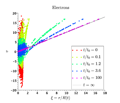
Figure 1: Snapshots of a subset of 3000 electrons in phase space. Initially, at time $t=0$, the electrons are distributed uniformly within a spherical shell $0.1<\xi<1$ with radial velocities following a Maxwell-Boltzmann distribution with thermal velocity $v_{\rm e}=8.34$ (cf equation (12).

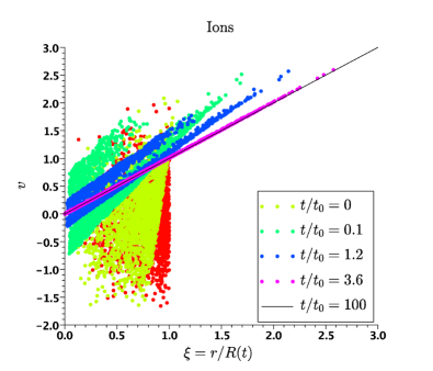
Figure 2: Snapshots of a subset of 3000 ions in phase space. Initially, at time $t=0$, the ions are distributed uniformly within a spherical shell $0.1<\xi<1$ with radial velocities following a Maxwell-Boltzmann distribution with thermal velocity $v_{\rm i}=0.834$ (cf equation (12).

Figures 1 and 2 show the motion in phase space of a fraction of electrons and ions from a numerical simulation of a spherical cloud expanding into vacuum. Positions and velocities of $N$ particles ($N/2$ electrons and $N/2$ ions) are time advanced according to equations (9) and (10) using a classical third order leap frog integration scheme [38]. The electric field is computed at every time step using the updated particles’ positions and the field equation (11).

The initial conditions consist in $N=80000$ particles uniformly distributed within the spherical shell $r_{\rm min}<r<R_{0}$ corresponding to $\Lambda=0.0538$. Thus, even though the simulated number of particles $N$ is much smaller than in a typical dust impact generated plasma cloud, it is still large enough for the key parameter $\Lambda$ to be much smaller than unity so that the expansion is quasi-neutral.

The inner sphere $r<r_{\rm min}$ cannot be penetrated by particles and is merely there to avoid the divergence of the Coulomb potential for $r\rightarrow 0$ when particles (actually thin spherical shells) approach the central region. In practice we chose $r_{\rm min}=0.1R_{0}$, which is both sufficiently small to minimise its influence on the overall system’s evolution and sufficiently large with respect to the strong interaction radius $r_{\rm s}$ to rule out binary collisions and self-charge effects.

In the following, if not otherwise stated, we normalise charge to the elementary charge e, mass to the electron mass $m_{\rm e}$, length to $r_{\rm min}$, electric field to $E_{\rm n}\equiv e/(4\pi\varepsilon_{0}r_{\rm min}^{2})$, velocities to $v_{\rm n}\equiv e/(m_{\rm e}4\pi\varepsilon_{0}r_{\rm min})^{1/2}$, time intervals to $t_{\rm n}\equiv r_{\rm min}/v_{\rm n}$ and temperatures to $T_{\rm n}\equiv m_{\rm e}v_{\rm n}^{2}$. With these normalisation, and by consistently normalising density to $r_{\rm min}^{3}$, the Debye length (1) reads $l_{\rm D}=(T/4\pi n)^{1/2}$, the mean free path (2) $l_{\rm e}=T^{2}/(\pi n\lambda)$ and the electric field of a point charge $Q$ becomes $E=Q/r^{2}$. We then set the initial temperature, for both electrons and ions, to $T_{0}=34.76$ and the cloud radius to $R_{0}=10$. The resulting Coulomb logarithm is then $\lambda=4.03$ and according to (2), the mean free path $l_{\rm e}$ is equal to $R_{0}=10$ as postulated. In code units the thermal velocity of the electrons is $v_{\rm e}=(2T_{0})^{1/2}=8.34$ and the strong interaction radius $r_{\rm s}=1/3T_{0}=9.6\>10^{-3}$ which, as required, is much smaller than both $R_{0}=10$ and $r_{\rm min}=1$.

For convenience in Figure 1 and in all subsequent figures we use normalised positions $\xi\equiv r/R(t)$ with the temporal variation of the scale length defined by $R(t)\equiv R_{0}(1+t/t_{0})$. We choose to set the arbitrary constant $t_{0}=10$ in order to have $d{R}/dt=1$. The ion to electron mass ratio is set to $m_{\rm i}/m_{\rm e}=100$ so that $t_{0}$ does actually turns out to be of the order of the ion sound crossing time $R_{0}/(3T/m_{\rm i})^{1/2}=9.8$, a characteristic time for the initial system. As already stated, at $t=0$ particles are uniformly distributed within the spherical shell $0.1<\xi\leq 1$ following Maxwell-Boltzmann velocity distributions for both ions and electrons:

$$f_{j}(v)=\frac{n_{0}}{\pi^{1/2}\>v_{j}}\>e^{-\displaystyle{(v/v_{j})^{2}}}$$ (12)

where $v_{j}=(2T_{0}/m_{j})^{1/2}$ is the thermal velocity of the corresponding species $\;j={\{\rm e,i\}}$.

4 Asymptotic evolution, theoretical background

The particle trajectories shown in Figures 1 and 2 illustrate two key aspects of the expansion which will be discussed in sections 4.1 and 4.2. First, as $t\rightarrow\infty$, all trajectories are seen to collapse towards the curve $v=\xi$. As a consequence the temperature at a given position $\xi$ is seen to decrease with time as the particles velocities appear to be less and less scattered as time progresses. Second, whereas ions rapidly line up in a structureless ribbon along the $v=\xi$ curve, electrons converge towards a more complex structure, also aligned on the $v=\xi$ curve, but with a bulging of the ribbon in the region $\xi\lesssim 2$. As we shall see below the bulging is due to the bouncing motion of electrons trapped in an electrostatic potential well.

4.1 Asymptotic convergence of particle trajectories

In this section we show that for $t\rightarrow\infty$ all particle trajectories must end up onto the $v=\xi$ curve provided the electric field decays sufficiently fast everywhere in the system. To this end we Taylor expand the asymptotic evolution of a particle velocity in terms of the small parameter $\nu=t_{1}/t\ll 1$, i.e. $v(\nu)=v(0)+\nu(\partial v/\partial\nu)_{\nu=0}$, where $t_{1}\gg t_{0}$ is just an arbitrary finite time level. From the equation of motion (9) we obtain the asymptotic evolution of a particle’s velocity

$$v(t\gg t_{1})=v_{\infty}-\frac{t^{2}}{t_{1}}\frac{qE(\xi,t)}{m}\bigg{|}_{t\rightarrow\infty}\left(\frac{t_{1}}{t}\right)=v_{\infty}-\frac{qE(\xi,t)t}{m}$$ (13)

where $v_{\infty}\equiv v(t=\infty)$. The asymptotic evolution of the particle’s position is formally obtained by integrating (10), i.e. $r(t)=r_{1}+\int_{t_{1}}^{t}v(\tau)d\tau$. Using $v(t)$ from equation (13), and for $t\gg t_{1}$ one obtains

$$\xi(t)=\frac{r_{1}}{t}+v_{\infty}-\frac{1}{t}\int_{t_{1}}^{t}d\tau\frac{qE(\xi,\tau)\tau}{m}.$$ (14)

The last term on the right hand side of equation (14) vanishes for $t\rightarrow\infty$ provided $E$ at position $\xi$ decays faster than $t^{-1}$ in which case $\xi_{\infty}\equiv\xi(t\rightarrow\infty)=v_{\infty}$, confirming that the end point of a particle’s trajectory lies on the $\xi=v$ curve. For a time dependence of the electric field $E\propto t^{\alpha}$ it is possible to compute the slope of a particle’s trajectory in the phase space directly from equations (13) and (14). Indeed, assuming that for $t\rightarrow\infty$ the variation of the electric field at a given particle position is due primarily to the time dependence of $E$ rather than to the particle’s motion, one obtains $(v-v_{\infty})/(\xi-\xi_{\infty})=2+\alpha$. Thus, for $\alpha=-2$, corresponding to the final, self-similar, evolution of our system (see Figure 8), $(v-v_{\infty})/(\xi-\xi_{\infty})=0$, i.e. trajectories approach the $\xi=v$ curve on horizontal trajectories with $v={\rm const}$. In the particular case where $E(\xi,t)=E_{1}(\xi)t_{1}^{2}/t^{2}$ (which applies to the simulation for $t/t_{0}\gg 1$) equations (13) and (14) reduce to

$$v = v_{\infty}-\frac{qE_{1}(\xi)}{m}\>\frac{t_{1}}{t}$$ (15)

$$\xi = \xi_{\infty}+\frac{r_{1}}{t}-\frac{qE_{1}(\xi)}{m}\>\frac{t_{1}}{t}\>\ln\left(\frac{t}{t_{1}}\right)\simeq\xi_{\infty}-\frac{qE_{1}(\xi)}{m}\>\frac{t_{1}}{t}\>\ln\left(\frac{t}{t_{1}}\right)$$ (16)

Equation (16) shows that for sufficiently late times $|\xi(t)-\xi_{\infty}|/\xi_{\infty}\ll 1$ confirming that the variation of the electric field at particle’s position is asymptotically dominated by the field decay and not by the particle’s motion. The interesting point about equation (16) is that it shows that for $t\rightarrow\infty$ (which allows neglecting the $r_{1}/t$ term) particles approach their final position $\xi_{\infty}$ from the left or the right depending on the sign of $qE_{1}$. Thus, in an overall positive electric field, which is indeed the case for the expanding cloud problem at hand (see Figure 8), ions approach their final position from the left in $(\xi,v)$ space while electrons approach their final position from the right. Thus, ions (electrons) which are initially on the right (left) of the $v=\xi$ curve will first cross the $v=\xi$ curve before converging towards their asymptotic position on horizontal $v\approx{\rm const}$ trajectories. This behaviour is already visible on the early phase of the expansion shown on figures 3 and 4.

4.2 Shrinking of the volume occupied by particles in $(\xi,v)$ space

The shrinking of the phase space volume occupied by the particles in the $(\xi,v)$ phase space is merely the consequence of the time dependence of the scaling length $R(t)$. The equations of motion for an individual particle (9) and (10) deriving from the general Hamiltonian of the system

$$H(r_{1},...,r_{N},p_{1},...,p_{N},t)=\sum_{j=1}^{N}p_{j}^{2}/2m_{j}+q_{j}\phi(r_{j},t)$$ (17)

where $p_{j}\equiv m_{j}v_{j}$ and $-\partial\phi/\partial r_{j}=E(r_{j},t)$, it follows that any volume $\Gamma=\int dvdr$ must be conserved along particle trajectories in $(v,r)$ space. Thus, $\Gamma=R(t)\int dvd\xi=const$ with the consequence that $\int dvd\xi\propto R(t)^{-1}=1/t$, i.e. the volume covered by the particles in the $(\xi,v)$ phase space shrinks in time as $1/t$. On the long term all particles must end up aligned on the $v=\xi$ curve with the spatial distribution of the charges being a function of the initial conditions, i.e. on the dimensionless parameter $\Lambda(N)\equiv\lambda_{D}/R_{0}$ only.

5 Trapping, bouncing and freezing of particle trajectories

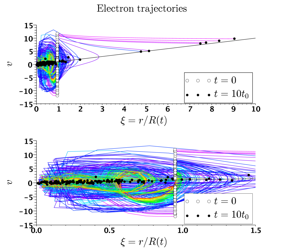
Figure 3: Sample trajectories of 102 electrons initially located in the range $0.949<\xi<0.95$ with velocities $-12<v<12$. The bottom panel is a zoom of the top panel.

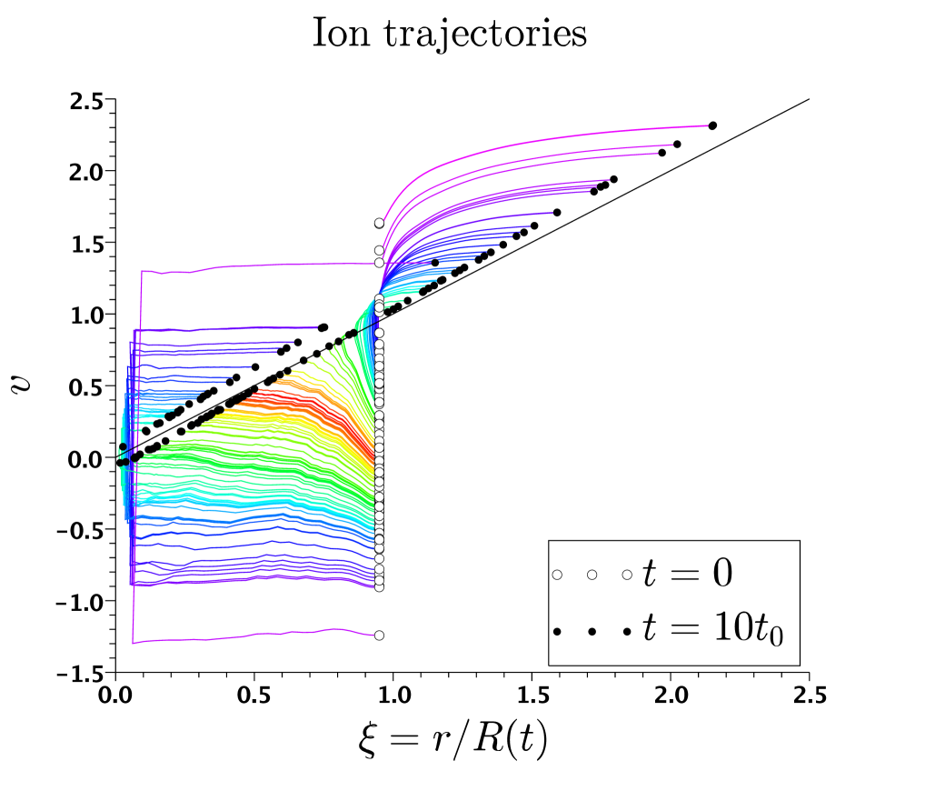
Figure 4: Sample trajectories of 116 ions initially located in the range $0.949<\xi<0.95$ with velocities $-2<v<2$.

Figures 3 and 4 show characteristic trajectories of selected electrons and ions in ($\xi,v$) phase space. From the figures it is immediately apparent that both species behave in a radically different way. Ions follow rather dull trajectories and are either accelerated outwards (in particular the outermost ones) or move at approximately constant velocity. The fastest electrons (in general the ones at largest radial distance $\xi$) are seen to steadily reduce their outflow velocity in the attractive field of the positively charged interior of the cloud. However, electrons, with sufficiently low initial energy (the ones with end velocity $v\lesssim 5$), do cross the $v=\xi$ curve and eventually bounce within an electrostatic trap. In order to understand the trajectories in the $(\xi,v)$ space it may be useful to rewrite the equations of motion (9) and (10) by setting $v=v(\xi(t))$, viz

$$(v-\xi)\frac{\partial v}{\partial\xi} = \frac{q}{m}E(\xi,t)\>t$$ (18)

$$\dot{\xi} = \frac{v-\xi}{t}$$ (19)

where we have used $dv/dt=\dot{\xi}\partial v/\partial\xi$ with $\xi=r/R(t)=r/t$ and $\dot{R}=1$. Equation (18) shows that when a trajectory crosses the $\xi=v$ it satisfies the condition $\partial v/\partial\xi=\infty$ (cf Figures 3 and 4) unless the electric field $E(\xi,t)=0$. In this particular case the particle’s velocity is constant $v=v_{\infty}$ and (19) shows that it takes an infinite time for the particle to reach the $v=\xi$ curve as $\xi(t)-\xi(\infty)\propto 1/t$. Multiple reflections are associated with an equal number of crossings of the $v=\xi$ curve, from top to bottom for an inward directed force and from bottom to top for an outward directed force. Note that particles approaching the centre $\xi=0$ make an artificial reflection there as their radial velocity must change from negative to positive. Given that in the simulations particles are not allowed to approach the centre at a distance less than $\xi_{\rm min}(t)=0.1R_{0}/R(t)$ reflection does effectively occur at $\xi_{\min}$ instead. Electrons bouncing back and forth in an expanding potential well can be efficiently cooled by first order Fermi deceleration. Now, despite the fact that both, bouncing and non bouncing electrons lose kinetic energy, the phase space volume occupied by the two populations evolves differently in time. Thus, whereas the velocity difference $\Delta v=|v_{2}-v_{1}|$ between two electrons with initial velocities $v_{2}$ and $v_{1}$ increases in time for $v_{1},v_{2}\gtrsim 10$, the opposite is true for the trapped (and eventually bouncing) electrons with initial velocities $v_{1},v_{2}\lesssim 10$ (see Figure 3). Loosely speaking, trapped electrons contribute to rise the particle concentration $f_{j}/\Delta v$ in velocity space while non trapped electrons, and basically all ions, contribute to reduce the particle concentration in velocity space. Both effects are visible in Figure 5 which shows that $f_{\rm e}(v)$ substantially grows over its initial value for $v\lesssim 1.5$ where Fermi deceleration occurs. For $v\gtrsim 1.5$ the electron trajectories in velocity space are divergent and $f_{\rm e}(v)$ falls below its initial value, instead.

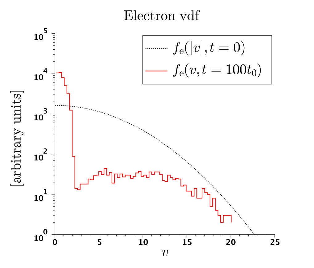
Figure 5: Electron velocity distribution function $f_{\rm e}(v)$ at the end of the simulation at $t=100t_{0}$. Plotted as a reference, the initial distribution of the absolute value of the radial velocities $f_{\rm e}(|v|)$.

A schematic representation of the electron dynamics in phase space and the corresponding evolution of their velocity distribution function $f_{\rm e}(t)$ summarising the discussion of this section is shown in Figure 6.

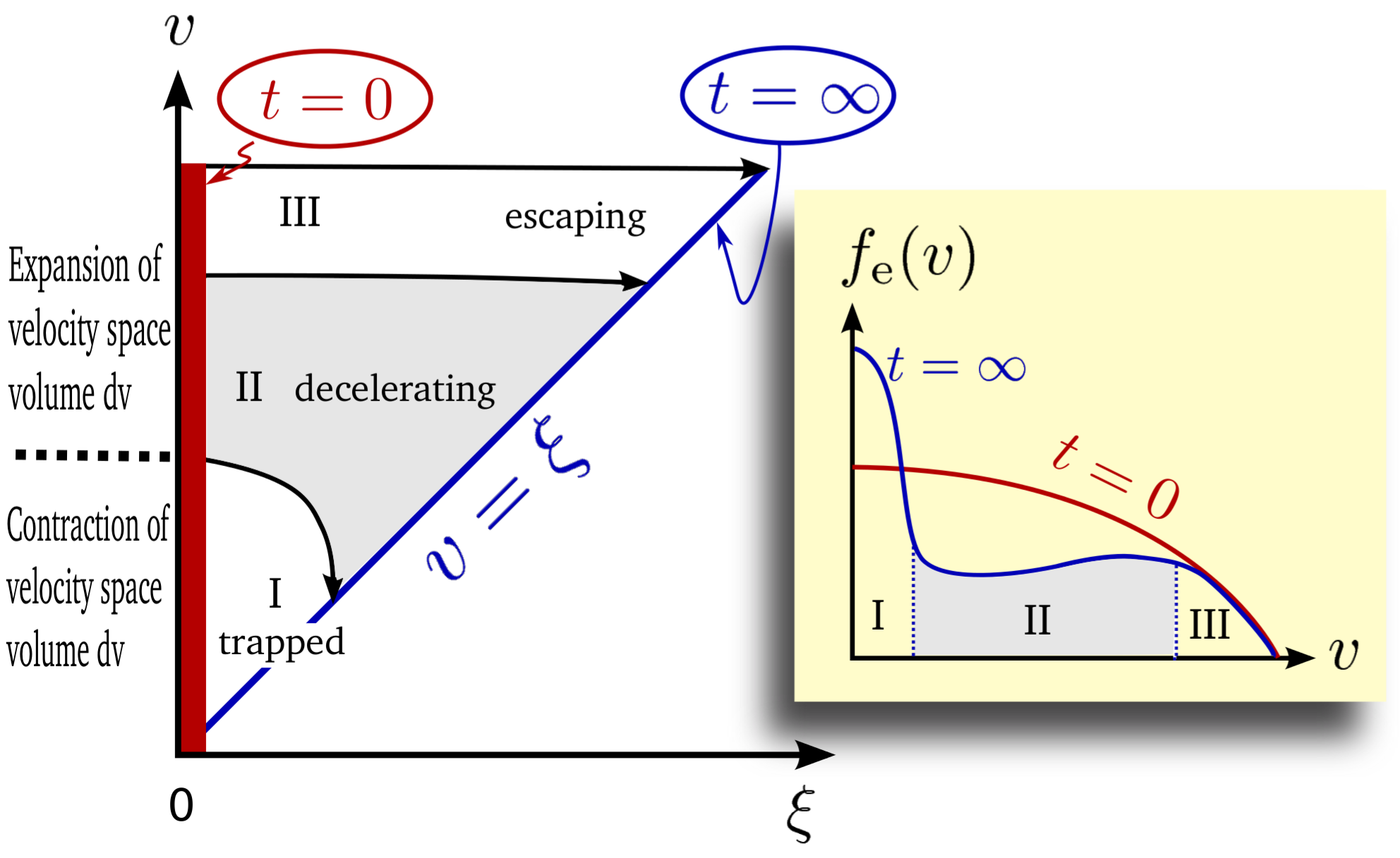
Figure 6: Schematic illustration of the electrons’ evolution in the $(\xi,v)$ phase space (left graph) and of the electron velocity distribution function $f_{\rm e}(v)$ (right graph).

5.1 Freezing of the bouncing motion

Figure 3 shows that some electrons have time to bounce several times during the simulation before their motion becomes frozen onto the $v=\xi$ curve. Others, for example the ones with initial velocity $v\approx 10$ and final velocity near $v\approx 3$ are unable to perform a full bounce period during the time of the simulation. The reason is that the bouncing period $t_{\rm b}$ for a particle of mass $m$ and charge $q$ moving in the potential $Q/r$ of a point charge $Q$ is of the order $t_{\rm b}\sim 2\pi(mr^{3}/qQ)^{1/2}$ (Kepler’s third law) so that $t_{\rm b}\propto\xi^{3/2}R^{3/2}\propto t^{3/2}$ grows faster than the expansion time $t_{\rm exp}=r/v=\xi R/v$. Thus, as the bouncing time to expansion time ratio $t_{\rm b}/t_{\rm exp}\sim 2\pi(v^{2}mR_{0}/qQ)^{1/2}\xi^{1/2}(R/R_{0})^{1/2}$ grows as $t^{1/2}$ the bouncing motion for a given particle will become frozen as soon as $t_{\rm b}(t,\xi,Q)/t$ exceeds a value of order unity. Electrons for which $t_{\rm b}/t_{\rm exp}\approx 1$ may just be a able to bounce once but may still lose a significant fraction of their initial kinetic energy if their total energy (kinetic + potential) is small and negative. A particle hitting a wall moving at velocity $w$ is slowed down by $\delta v=-2w$ or $\delta v=2(w-v)$ depending on whether its initial velocity $v$ is in the range $v\geq 2w$ or $2w>v>w$, respectively. Given that the expansion velocity of the electrostatic walls is rather slow compared to the electron thermal velocity $v_{\rm e}=8.3$ (the peak of the electrostatic profile in Figure 8 at $\xi\gtrsim 2$ moves outwards at a velocity $\lesssim 2$), 2 or 3 reflections are required to slow down a thermal electron below the critical velocity $v^{*}\approx 2$ which separates bouncing and non bouncing electrons (see Figures 5 and 6). The maximum initial velocity $v^{*}$ of a trapped electron can be estimated by equating the bouncing period $t_{\rm b}$ and the expansion time $t_{\rm exp}=\xi R/v$

$$v^{*}\approx\frac{R^{-1/2}}{2\pi}\left[\frac{Q(\xi)}{\xi}\right]^{1/2}.$$ (20)

Equation (20) may appear rather useless, $Q(\xi)$ being an unknown function of $\xi$. However, we expect the right hand side of equation (20) to be largest after a short time of the order $\lambda_{\rm D}/v_{\rm e}=0.091$ (the inverse electron plasma frequency) from the beginning of the simulation. Thus, an a priori estimate is possible if we assume that $Q$ corresponds to the number of electrons in the outer Debye shell of the initial cloud, i.e. $Q\approx 4\pi\lambda_{\rm D}R_{0}^{2}n_{\rm e}=1.5N\Lambda$. In the present case $N=80000$ and $\Lambda=0.0538$ so that $Q\approx 6456$. With these numbers and by setting $R=R_{0}=10$ and $\xi=1$ in equation (20), one obtains $v^{*}\approx 4$ which appears to be a fair estimate of the upper limit for the initial velocity of trapped electrons (see Figure 3).

5.2 Ion distribution

The asymptotic ion velocity distribution is shown in Figure 7. The figure clearly shows that the ion distribution closely follows the electron distribution for $v\lesssim 1.7$ (roughly twice the ion thermal velocity $(2T_{0}/m_{\rm i})^{1/2}=0.83$) while at higher velocities, up to the velocity of the fastest ions in the simulation $v\approx 2.5$, the ion density is in excess over the electron density. On the other hand, for $v\lesssim 0.5$ the asymptotic distribution $f_{\rm i}(v,\infty)$ falls below its initial value $f_{\rm i}(v,0)$ while the opposite occurs for $v\gtrsim 0.5$. In principle, given that the mobile electrons tend to escape from the cloud, all ions should be accelerated outwards by the positive charge $Q(\xi)$ of the remnant (see bottom panel of Figure 9) and its associated, outwards directed electric field (see Figure 8). The outwards directed force should produce a displacement towards larger radial velocities of the original velocity distribution $f_{\rm i}(|v|,0)$ with $f_{\rm i}(|v|,t)=0$ below some minimum velocity. The displacement of $f_{\rm i}$ towards higher radial velocity is visible in 7 for the fastest ions with end velocities $v\gtrsim 0.5$. However, no region with $f_{\rm i}=0$ is visible at low velocities, though. The reason is that the slow ions are kept in the inner part of the cloud by the inwards falling, Fermi decelerated, electrons. The coupling between ions and cold electrons is so efficient there that the electric field asymptotically goes to zero for $\xi\lesssim 1.5$ (see Figure 8).

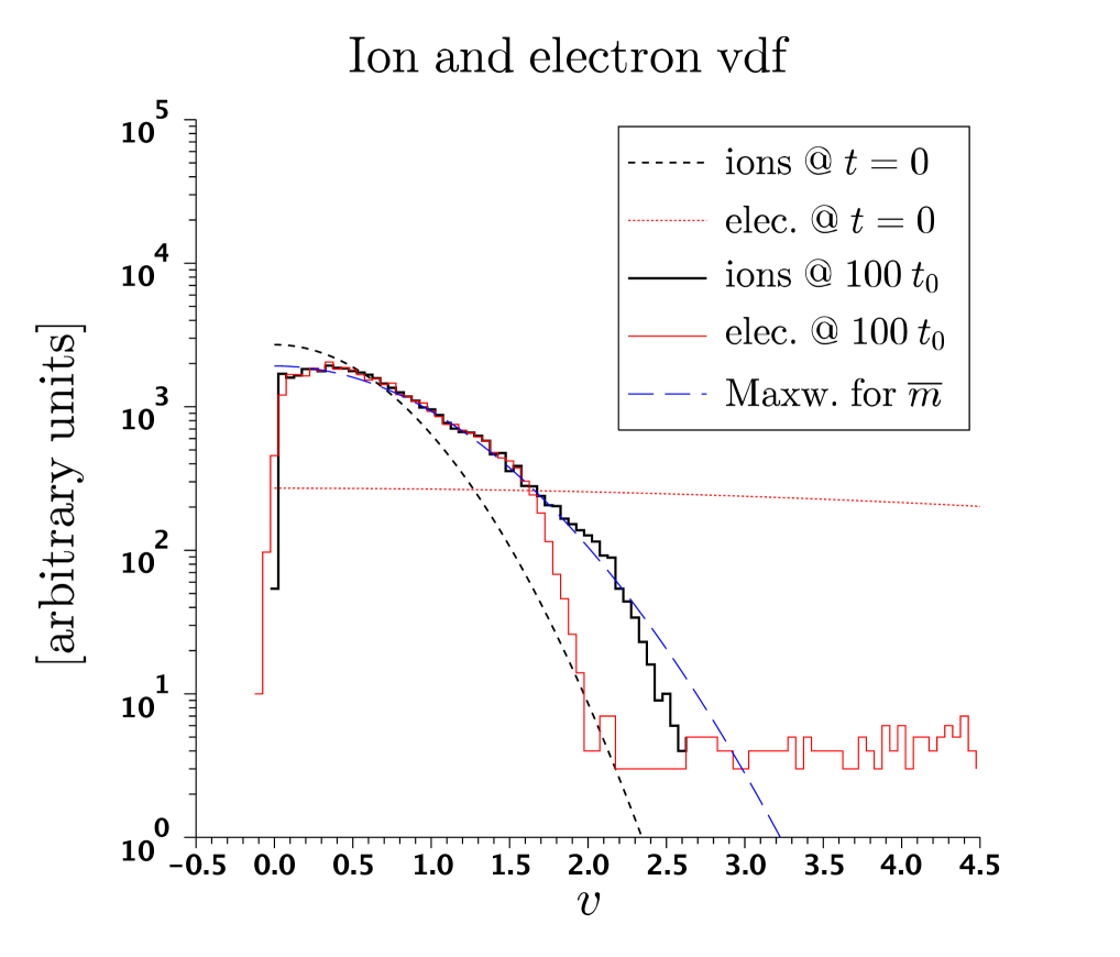
Figure 7: Ion and electron velocity distributions $f_{k}(v)$ at the end of the simulation at $t=100t_{0}$. Also plotted are the initial distributions $f_{k}(|v|,0)$ and the Maxwellian $N(\pi v_{\overline{m}})^{-1/2}\exp[-(v/v_{\overline{m}})^{2}]$ where $v_{\overline{m}}\equiv(2T_{0}/\overline{m})^{1/2}=1.17$ is the thermal velocity based on the initial temperature $T_{0}=34.76$ and a particle of mass $\overline{m}\equiv(m_{\rm i}+m_{\rm e})/2=50.5$.

Figure 7 also shows that up to $v\approx 1.7$ both electron and ion velocity distributions are conveniently fitted by a single Maxwellian distribution with thermal speed $v_{\overline{m}}=(2T_{0}/\overline{\rm m})^{1/2}=1.17$ where $\overline{m}\equiv 0.5(m_{\rm i}+m_{\rm e})=50.5$ is the average particle mass. If we assume that the electron distribution is a Maxwellian sharply cut at an upper velocity $v^{*}$, such that the missing electrons are those in the outer Debye shell of the initial sphere $1.5\Lambda N=6456$, we obtain the estimate ${\rm Erf}(v^{*}/v_{\overline{m}})=1-1.5\Lambda$ (where ${\rm Erf}(x)\equiv 2\pi^{-1/2}\int_{0}^{x}ds\>\exp(-s^{2})$ is the error function) which gives $v^{*}=1.44$. Obviously, $1.5\Lambda N$ is an overestimate of the number of electrons in the electron precursor. From Figure 9 we take that this number is roughly 5 times smaller than $1.5\Lambda N$ which allows for a more realistic estimate ${\rm Erf}({v^{*}}/v_{\overline{m}})=1-1.5\Lambda/5$, i.e. $v^{*}=1.99$.

6 Charge distribution and electric field

The spatial and temporal structure of the electric field is shown in Figure 8.

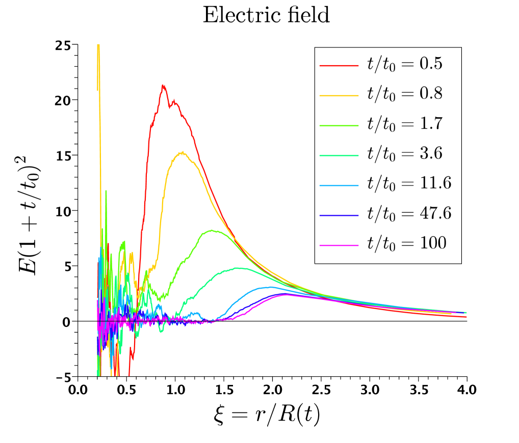
Figure 8: Temporal evolution of the electric field profile. For $t\gtrsim 30$ the spatial profile is essentially frozen while the amplitude declines $\propto t^{-2}$.

As expected, after a dynamic initial phase, when particles are close to their asymptotic position in the $(\xi,v)$ space, the electric field intensity decays as $E({\xi,t})\propto t^{-2}$. The spatial structure $E(\xi,\infty)$ is characterised by a central region $\xi\lesssim 1$ where, apart from fluctuations due to the small number of particles , the field intensity is essentially zero, corresponding to the region where the electron and ion density are equal (see Figure 9). For $\xi\gtrsim 1.6$ the field intensity rapidly rises towards the maximum $E_{\max}(1+t/t_{0})^{2}\approx 2.5$ at $\xi=2.1$, followed by a gentler negative slope over a much larger spatial scale. The large scale is associated with the scale of the electron precursor, which is obviously forged by the initial electron velocity distribution, and scales as $\xi_{\rm fall}\approx v_{\rm e}t_{0}/R_{0}=8.34$. The shorter scale of the rising part of the field profile is forged by the ions and scales as $\xi_{\rm rise}\approx v_{\rm i}t_{0}/R_{0}=0.83$.

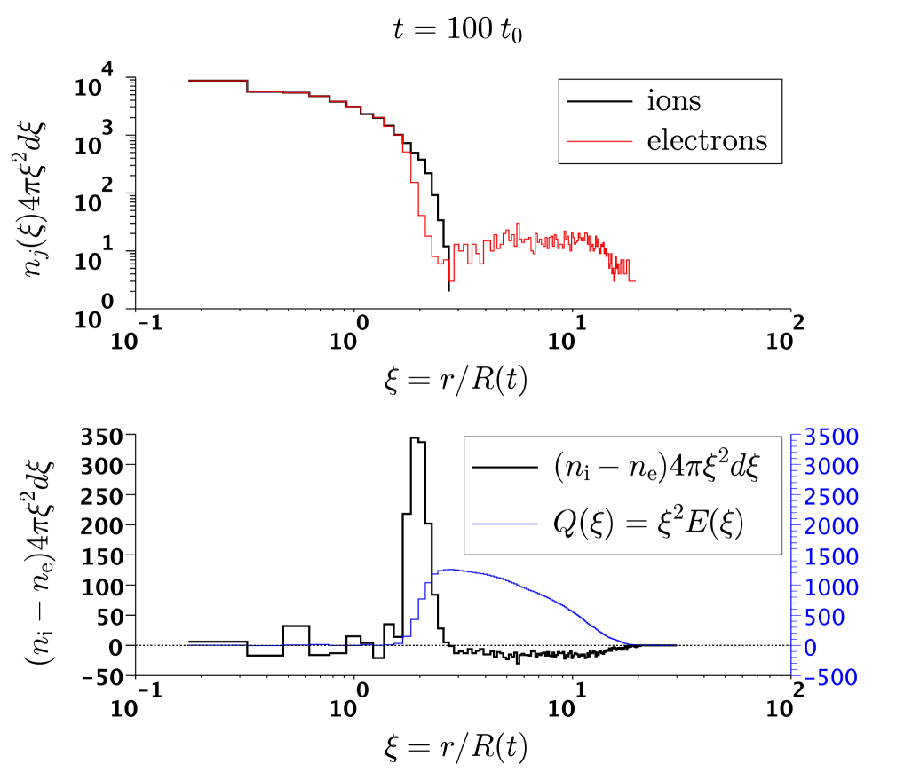
Figure 9: Radial linear density for ions and electrons (top panel). The bottom panel shows the linear charge density (thick black curve and right scale) in units of the positive elementary charge $|e|$. The thin blue curve corresponds to the net charge $Q(\xi)$ contained within the the spherical shell of radius $\xi$.

The charge distribution at the end of the simulation at $t=100t_{0}$ is shown in the bottom panel of Figure 9 where, again, $Q(\xi)$ represents the charge within the sphere of radius $\xi$. The maximum $Q_{\rm max}\approx 1292$ is reached for $\xi\approx 2.7$. Thus $Q_{\rm max}\approx 0.3N\Lambda$, corresponding to roughly $1/5$ of the positive charge contained in the outermost Debye shell of the cloud at $t=t_{0}$. On the other hand the charge at the position of the electric field maximum is $Q(\xi=2.1)\approx 1053\approx 0.245N\Lambda$ giving a maximum field intensity $E_{\max}(t/t_{0})^{2}\approx 0.245N\Lambda/(2.1R_{0})^{2}\approx 2.4$ as confirmed by the latest profiles of $E$ shown in Figure 8. Changing to SI units we obtain a more useful expression

$$E_{\max,{\rm SI}}=8\>10^{-11}\frac{N\Lambda}{R^{2}}$$ (21)

where $E_{\max,{\rm SI}}$ is expressed in V/m and $R$ in metres.

7 Ion and electron fluid velocities

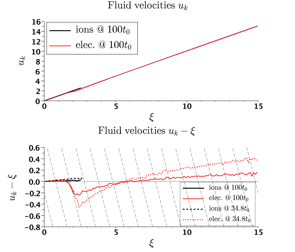
Figure 10: Fluid velocities $u_{j}(\xi)=\int_{-\infty}^{\infty}v\>f_{j}(v,\xi)dv/n_{j}{\xi}$ for ions and electrons at the end of the simulation (top panel) and $u_{j}-\xi$ for at two different times (bottom panel). The grid of dashed lines in the bottom panel gives the trajectories $v={\rm const}$ individual particles are expected to follow in case of an electric field declining as $t^{-2}$ (see Section 4.1).

Figure 10 shows the spatial fluid velocity profiles $u_{\rm e,p}$ for both electron and ions at the end of the simulation. Not surprisingly both populations have velocities profiles close to the $v=\xi$ curve (top panel). Plotting the fluid velocities $u_{\rm e,p}-\xi$ versus $\xi$ (bottom panel) shows that while all ions and electrons located within $\xi\lesssim 1.7$ do closely follow the $v=\xi$ curve (meaning that they are already frozen) electrons with $1.7\lesssim\xi\lesssim 6$ stay below the $v=\xi$ curve. These electrons are still flowing (falling) inwards along the dashed lines, corresponding to the $v={\rm const}$ trajectories predicted for a $t^{-2}$ declining electric field (see Section 4.1). The electron inflow velocity at $t=100t_{0}$ peaks near $\xi\approx 2.3$ at about $10\%$ of the absolute ion fluid velocity. The ion velocity will not evolve significantly after $t=100t_{0}$ as it is already well approximated by $u_{\rm i}=\xi$. The asymptotic position of the electrons near $\xi\approx 2$ at $t=100t_{0}$, will lie some $10\%$ closer to the centre of the cloud. This late displacement of the electrons will not modify the final structure of the electric field significantly as the density of these inflowing electron is substantially lower than the ion density near $\xi=2$ (see Figure top panel in 9). On the other hand, electrons at $\xi(100t_{0})\gtrsim 3$ are too fast for the ions to catch up with and constitute the final electron precursor.

8 Application to the case of clouds formed by interplanetary nanoparticles impacts

When dust particles travelling in the interplanetary space hit a solid object at characteristic velocities of the order of tens to hundreds km/s, a plasma cloud is generated at the impact point. The cloud is formed due to the vaporisation and partial ionisation of the dust particle itself and the target material. The subsequent expansion of the cloud is hemispherical rather then spherical as assumed in the above model. In the case of a non conducting and charge neutral target the above results should not be modified in any substantial way. On the other hand, one should be extremely cautious when trying to interpret the electric signals measured on a spacecraft as spacecraft are generally positively charged due to electrons being stripped from their metallic surface through photoionisation by solar radiation. The associated electric field (typically of the order of a few V/m) exceeds the cloud’s internal electric field very early during the expansion, causing stripping of most of the cloud’s electrons [17]. Not only is the expanding cloud subject to charging so that the long term expansion is more like a Coulomb explosion[1, 27] rather than a quasi-neutral expansion as described above, but the role of the photoelectrons, continually emitted and recollected by the spacecraft, must be taken into account when trying to interpret the voltage pulses measured on spacecraft antennae. Indeed, in the scenario described in appendix A of the Zaslawsky et al paper [39]), the voltage pulses measured on individual antennae in conjunction with the impact of nano dusts on the STEREO spacecraft are not a direct measure of the field within the post impact expanding plasma cloud but are the consequence of the equilibrium photoelectron return current towards the part of the antenna within the plasma cloud being interrupted. The interruption of the photoelectron return current induces an accumulation of positive charges on the antenna which is then measured by on board detectors as a temporal variation of the potential between the antenna and the spacecraft.

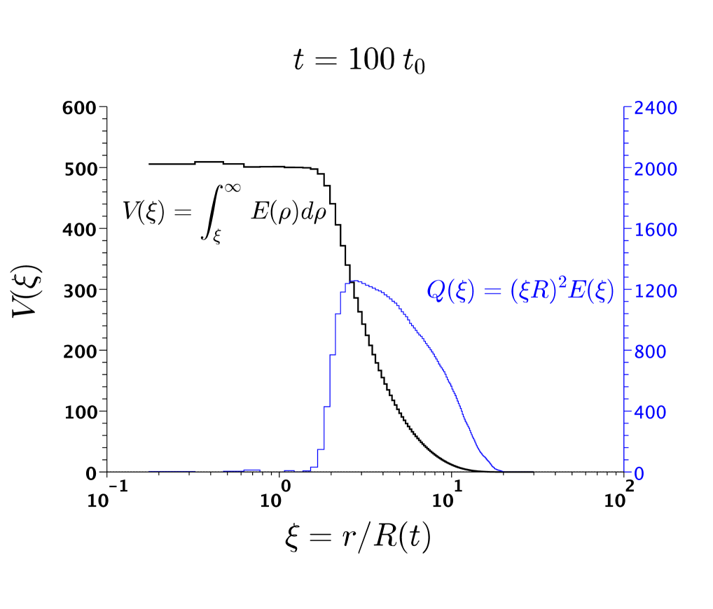
Figure 11: Electrostatic potential $V(\xi)$ and total charge $Q(\xi)$ as in figure 9.

Let us estimate the electrostatic potential through a real cloud generated by a nanoparticle hitting a target in interplanetary space using the above model. As we shall see the intrinsic field of the cloud is too weak to account for the impact associated potential pulses observed on STEREO.

The electrostatic potential through the simulated plasma cloud is shown in Figure 11. The total drop in the electrostatic potential is $\Delta V\approx 550$ while, as already stated, the peak charge is $Q_{\rm max}\approx 1292$ (see bottom panel in Figure 9). Assuming a linear relation between $\Delta V$ and $Q_{\rm max}$ we find

$$\Delta V(N)\approx{Q_{\rm max}\over 2.35}\approx 0.128~{}N\Lambda~{}~{}~{}({\rm simulation~{}~{}units}).$$ (22)

This relation can be interpreted as the electrostatic potential at the surface of a sphere of radius $2.35R$ enclosing a charge $Q_{\rm max}$. Multiplication of Equation (22) by $e/(4\pi\varepsilon_{0}R)$ in SI units, leads to the dimensional version of (22):

$$\Delta V_{\rm SI}(N,R)\approx 1.84~{}10^{-10}\;{{N\Lambda}\over R}$$ (23)

where $R$ is in meters and $V_{\rm SI}$ in Volts.

Let us use equation (23) to estimate the voltage pulse $\Delta V$ due to the impact of a $m_{\rm d}=10^{-20}\,$kg grain (size $\sim 10\,$nm) travelling at $v=300\,$km/s. The number of electrons and ions within the plasma cloud can be estimated via the semi-empirical formula $N/2\approx 0.7m_{\rm d}^{1.02}v^{3.48}/e$ (see [17, 31]), where $[e]={\rm C}$, $[m_{\rm d}]=$kg and $[v]=$km/s. With these parameters we obtain $N\approx 1.4~{}10^{7}$ and, from the relation between $\Lambda$ and $N$ established in the discussion following equation (4) we find $\Lambda(1.4~{}10^{7})=0.016$. Plugging this value into in equation (23) leads to $\Delta V_{\rm SI}(1.4~{}10^{7})\approx 4.1~{}10^{-5}/R$. Thus, when the cloud’s radius has grown to $R=50$cm, i.e. when its density has fallen to a value comparable to the interplanetary density, $\Delta V_{\rm SI}\approx 0.082{\rm mV}$ only. Noting that the effectively measured voltage is obtained by averaging over the whole antenna length, i.e. by multiplying the above voltage by $l/L$, where $L$ is the length of the antenna (6 m on STEREO) and $l$ the length of the part of the antenna within the cloud, the voltage predicted by the model is far too week to be directly detectable and in any case much too weak to induce the up to 100mV pulses observed on STEREO. Previous estimates of the voltage pulse associated with nano-size dust impacts were based on the assumption that the charge separation within the expanding cloud is total with $\sim N/2$ electrons in the precursor[17]. The assumption, adopted here, that charge separation only occurs at the time when the expanding cloud becomes collisionless, without influence of potential external fields, reduces the number of electrons in the precursor to a much smaller number of order $0.3N\Lambda$. Using equation (21) we can estimate the maximum electric field within the above cloud to be of order $E_{\max,SI}\approx 1.8\;10^{-5}R^{-2}$. Thus, when the cloud has reached $R=4.2{\rm mm}$ the maximum field is already down to 1V/m, i.e. comparable to the spacecraft’s own field. Beyond this size, the cloud will start loosing its electrons to the spacecraft. However, even in case of a complete charge separation such that the electrostatic field outside the cloud is given by the Coulomb field $Q/r$, the latter is much too weak (at most a few mV) to account for the on board measured voltage pulses associated with nanodust impacts. As we shall explain in more details in a forthcoming paper, but as already briefly exposed in the appendix A of [39], the strong potential pulses measured on individual antennas on STEREO are due to the perturbative effect of the expanding cloud on the photoelectrons surrounding the antenna.

9 Summary and conclusions

We have explored numerically the unconstrained spherically symmetric expansion of an initially uniform, overall neutral and at thermodynamic equilibrium cloud of immobile plasma. The initial temperature and density of the plasma are such that the cloud’s radius equals the Fokker-Planck collisional mean free path of a thermal electron, representing an admittedly crude model of an expanding cloud at the time it becomes collisionless. Consistently assuming that the ion and electron velocity distributions are Maxwellians at the time of the collisional to collisionless transition, it follows that the key parameter of the problem $\Lambda\equiv\lambda_{\rm D}/R_{0}$ can be written as a function of the total number of ions and electrons in the cloud only. Due to the $\Lambda\propto N^{-1/4}$ dependence (see equation (4)) typical nano size grain impacts which are expected to ignite plasma clouds with $N=\mathcal{O}(10^{8})$, $\Lambda$ is always much smaller then unity, i.e. the collisionless expansion is quasi-neutral.

During the initial phase of the collisionless regime most electrons (the less energetic ones) lose nearly all of their kinetic energy thorough Fermi deceleration in the expanding potential (see Figure 11). On the other hand the outermost ions near the electric field maximum (see Figure 8), are accelerated outwards by the positive electric field. The net effect is that ions and electrons do asymptotically tend towards having the same velocity distribution up to a threshold of the order of the ion thermal velocity (see Figure 7). The fact that all particle trajectories converge towards the $v=\xi$ curve as $t\rightarrow\infty$ implies that electron and ion fluid velocities end up being simple linear functions of the distance $r$ from the expansion centre.

At late times the ion density profile is conveniently described by $n_{\rm i}(r)\propto\exp[-(r/tv_{\overline{m}})^{2}]$ where $v_{\overline{m}}\equiv(2T_{0}/\overline{m})^{1/2}$ is the thermal velocity based on the initial temperature $T_{0}$ and the mean mass $\overline{m}\equiv 0.5(m_{\rm i}+m_{\rm e})$. Because of $\Lambda\ll 1$ the electron density $n_{\rm e}$ closely follows the ion density up to a distance $r^{*}$ solution of the equation ${\rm Erf}(r^{*}/tv_{\overline{\rm m}})\approx 1-0.3\Lambda N$. Beyond this point the electron density is flat up to a radial distance of the order of $v_{\rm e}t$ as observed in Vlasov simulations [29]. The electric field is essentially zero for $r\lesssim r^{*}$ (see Figure 8) but rises towards a maximum on the ion length scale $r_{\rm rise}\approx v_{\rm i}t$ and decreases slowly on the electron precursor length scale $r_{\rm fall}\approx v_{\rm e}t$. At late times the maximum field intensity $E_{\rm max}$ is essentially nailed down by the number of electrons in the outer shell of the cloud of thickness $\lambda_{\rm D}$. This number can be expressed in terms of the total number of particles $N$ and the dimensionless parameter $\Lambda\equiv\lambda_{\rm D}/R_{0}$ to give $1.5N\Lambda$, implying that the electric field intensity must be proportional to $N\Lambda/R^{2}$. In our representative simulation, we find $E_{\max,{\rm SI}}\approx 8\>10^{-11}N\Lambda/R^{2}$ which we expect to hold as long as $N\gg 1$ and provided the cloud has changed from collisional to collisionless during expansion. The electrostatic potential through the cloud has been found to be $\Delta V_{\rm SI}(N,R)\approx 1.84~{}10^{-10}N\Lambda/R$.

The electrostatic potential difference between the cloud’s centre and infinity predicted by the model is far too weak to be account for the voltage pulses,sometimes exceeding 100mV, observed on the S/WAVES TDS detector on the STEREO spacecraft following a nano-sized dust particles impact. One plausible reason for this discrepancy is that spacecraft are positively charged due to photoelectron emission through their sunlight exposed surfaces. The resulting electric field, typically of the order of a few $V{\rm m}^{-1}$ at 1AU from the Sun, generally exceeds the maximum field intensity within the plasma cloud before its dilution in the ambient plasma. The late evolution of the cloud is therefore dominated by the spacecraft field which strips most or all of the electrons from the cloud which then sees both its charge and its internal electrostatic potential field increase by a factor of order $\Lambda^{-1}\gg 1$. However, even in case of an unrealistically large nanodust impact generated cloud with some $N=10^{8}$ and with all electrons stripped-off, the total electrostatic potential difference would merely be a smallish $20{\rm mV}$ at the time of its maximum extension, when $R\approx 1{\rm m}$. Considering that the measured field is down by at least a factor $R/L$, where $L$ is the the total length of the antenna ($L=6{\rm m}$ on the Stereo spacecraft), one must conclude that the on board measured fields are not a direct measure of the cloud’s intrinsic field. Indeed, recent findings by Zaslavsky et al [39] indicate that nanodust impact associated clouds strongly affect the photoelectron environment of the antenna. In the scenario proposed by Zaslavsky et al the photoelectrons emitted by the sunlight exposed surface of the antenna are temporarily hindered to fall back onto it because of the presence of the cloud’s perturbing field. The resulting net photoelectron current is strong enough to allow for a fast positive charging of the antenna which is compatible with the measured field intensities. The bottom line is that the presented model is not directly applicable to the case of plasma clouds generated by nanodust impacts on spacecraft as neither the spacecraft potential nor the surrounding photoelectrons have been considered. The model is however expected to be applicable in case of nanodust impacts on uncharged targets.

References

References

- [1] F. Peano, J. L. Martins, R. A. Fonseca, L. O. Silva, G. Coppa, F. Peinetti, and R. Mulas. Dynamics and control of the expansion of finite-size plasmas produced in ultraintense laser-matter interactions. Physics of Plasmas, 14:6704–+, May 2007.
- [2] T. Ditmire, J. Zweiback, V. P. Yanovsky, T. E. Cowan, G. Hays, and K. B. Wharton. Nuclear fusion from explosions of femtosecond laser-heated deuterium clusters. Nature, 398:489–492, April 1999.
- [3] S. Ter-Avetisyan, M. Schnürer, H. Stiel, U. Vogt, W. Radloff, W. Karpov, W. Sandner, and P. V. Nickles. Absolute extreme ultraviolet yield from femtosecond-laser-excited xe clusters. Phys. Rev. E, 64(3):036404–+, September 2001.
- [4] Y. Kishimoto, T. Masaki, and T. Tajima. High energy ions and nuclear fusion in laser-cluster interaction. Physics of Plasmas, 9:589–601, February 2002.
- [5] P. Mora. Thin-foil expansion into a vacuum. Physical Review E, 72(5):056401–+, November 2005.
- [6] B. N. Breizman, A. V. Arefiev, and M. V. Fomyts’kyi. Nonlinear physics of laser-irradiated microclusters. Physics of Plasmas, 12(5):056706–+, May 2005.
- [7] K. E. Lonngren. Expansion of a dusty plasma into a vacuum. Planetary and Space Science, 38:1457–1459, November 1990.
- [8] S. R. Pillay, S. V. Singh, R. Bharuthram, and M. Y. Yu. Self-similar expansion of dusty plasmas. Journal of Plasma Physics, 58:467–474, October 1997.
- [9] P. C. Birch and S. C. Chapman. Two dimensional particle-in-cell simulations of the lunar wake. Physics of Plasmas, 9:1785–1789, May 2002.
- [10] D. A. Gurnett, E. Grun, D. Gallagher, W. S. Kurth, and F. L. Scarf. Micron-sized particles detected near saturn by the voyager plasma wave instrument. Icarus, 53:236–254, February 1983.
- [11] M. G. Aubier, N. Meyer-Vernet, and B. M. Pedersen. Shot noise from grain and particle impacts in saturn’s ring plane. Geophys. Res. Lett., 10:5–8, January 1983.
- [12] N. G. Utterback and J. Kissel. Attogram dust cloud a million kilometers from comet halley. Astronomical Journal, 100:1315–1322, October 1990.
- [13] H. A. Zook, E. Grun, M. Baguhl, D. P. Hamilton, G. Linkert, J.-C. Liou, R. Forsyth, and J. L. Phillips. Solar wind magnetic field bending of jovian dust trajectories. Science, 274:1501–1503, November 1996.
- [14] N. McBride and J. A. M. McDonnell. Meteoroid impacts on spacecraft:sporadics, streams, and the 1999 leonids. Planetary and Space Science, 47:1005–1013, August 1999.
- [15] I. Mann and A. Czechowski. Dust destruction and ion formation in the inner solar system. Astrophysical Journal Letters, 621:L73–L76, March 2005.
- [16] S. Kempf, R. Srama, M. Horányi, M. Burton, S. Helfert, G. Moragas-Klostermeyer, M. Roy, and E. Grün. High-velocity streams of dust originating from saturn. Nature, 433:289–291, January 2005.
- [17] N. Meyer-Vernet, M. Maksimovic, A. Czechowski, I. Mann, I. Zouganelis, K. Goetz, M. L. Kaiser, O. C. St. Cyr, J.-L. Bougeret, and S. D. Bale. Dust detection by the wave instrument on STEREO: nanoparticles picked up by the solar wind? Solar Physics, 256:463–474, May 2009.
- [18] O. C. St. Cyr, M. L. Kaiser, N. Meyer-Vernet, R. A. Howard, R. A. Harrison, S. D. Bale, W. T. Thompson, K. Goetz, M. Maksimovic, J.-L. Bougeret, D. Wang, and S. Crothers. STEREO SECCHI and S/WAVES observations of spacecraft debris caused by Micron-Size interplanetary dust impacts. Solar Physics, 256:475–488, May 2009.
- [19] Ya. B. Zel’dovich and Yu. P. Raizer. Physics of shock waves and high-temperature hydrodynamic phenomena. Courier Dover Publications, 2002.
- [20] D. C. Pack. The motion of a gas cloud expanding into a vacuum. Monthly Notices of the Royal Astronomical Society, 113:43, 1953.
- [21] K. P. Stanyukovich. Unsteady motion of Continuous Media. Pergamon Press, 1960.
- [22] Y. Tzuk, B. D. Barmashenko, I. Bar, and S. Rosenwaks. The sudden expansion of a gas cloud into vacuum revisited. Physics of Fluids, 5:3265–3272, December 1993.
- [23] C. Sack and H. Schamel. Plasma expansion into vacuum - a hydrodynamic approach. Physics Reports, 156:311–395, December 1987.
- [24] P. Mora. Plasma expansion into a vacuum. Physical Review Letters, 90(18):185002–+, May 2003.
- [25] M. Murakami and M. M. Basko. Self-similar expansion of finite-size non-quasi-neutral plasmas into vacuum: Relation to the problem of ion acceleration. Physics of Plasmas, 13:2105–+, January 2006.
- [26] N. Kumar and A. Pukhov. Self-similar quasineutral expansion of a collisionless plasma with tailored electron temperature profile. Physics of Plasmas, 15(5):053103–+, May 2008.
- [27] A. Beck and F. Pantellini. Spherical expansion of a collisionless plasma into vacuum: self-similar solution and ab initio simulations. Plasma Physics and Controlled Fusion, 51(1):015004–+, January 2009.
- [28] F. Peano, F. Peinetti, R. Mulas, G. Coppa, and L. O. Silva. Kinetics of the collisionless expansion of spherical nanoplasmas. Physical Review Letters, 96(17):175002–+, May 2006.
- [29] G. Manfredi, S. Mola, and M. R. Feix. Rescaling methods and plasma expansions into vacuum. Physics of Fluids B, 5:388–401, February 1993.
- [30] D. S. Dorozhkina and V. E. Semenov. Exact Solution of Vlasov Equations for Quasineutral Expansion of Plasma Bunch into Vacuum. Physical Review Letters, 81:2691–2694, September 1998.
- [31] K. Hornung and J. Kissel. On shock wave impact ionization of dust particles. Astronomy and Astrophysics, 291:324–336, November 1994.
- [32] P. Molmud. Expansion of a rarefield gas cloud into a vacuum. Physics of Fluids, 3:362–366, May 1960.
- [33] L. Spitzer and R. Härm. Transport phenomena in a completely ionized gas. Physical Review, 89:977–981, 1953.
- [34] L.D. Landau and E.M. Lifshits. Fluid mechanics. 2nd ed. Volume 6 of Course of Theoretical Physics. Transl. from the Russian by J. B. Sykes and W. H. Reid. Pergamon Press, 1987.
- [35] E. C. Shoub. Invalidity of local thermodynamic equilibrium for electrons in the solar transition region. i - Fokker-Planck results. The Astrophysical Journal, 266:339–369, March 1983.
- [36] J. F. Luciani, P. Mora, and J. Virmont. Nonlocal heat transport due to steep temperature gradients. Phys. Rev. Lett., 51(18):1664–1667, October 1983.
- [37] C. Salem, D. Hubert, C. Lacombe, S. D. Bale, A. Mangeney, D. E. Larson, and R. P. Lin. Electron properties and coulomb collisions in the solar wind at 1 AU: <i>Wind</i> observations. The Astrophysical Journal, 585(2):1147–1157, March 2003.
- [38] G. D. Quinlan and S. Tremaine. Symmetric multistep methods for the numerical integration of planetary orbits. Astronomical Journal, 100:1694–1700, November 1990.
- [39] A. Zaslavsky, N. Meyer-Vernet, I. Mann, A. Czechowski, K. Issautier, G. Le Chat, F. Pantellini, K. Goetz, M. Maksimovic, S. D. Bale, and J. C. Kasper. Interplanetary dust detection by radio antennas: Mass calibration and fluxes measured by STEREO/WAVES. sumitted to "Journal of Geophysical Research - Space Physics", 2011.