New implementation of hybridization expansion quantum impurity solver based on Newton-Leja interpolation polynomial

Abstract

We introduce a new implementation of hybridization expansion continuous time quantum impurity solver which is relevant to dynamical mean-field theory. It employs Newton interpolation at a sequence of real Leja points to compute the time evolution of the local Hamiltonian efficiently. Since the new algorithm avoids not only computationally expansive matrix-matrix multiplications in conventional implementations but also huge memory consumptions required by Lanczos/Arnoldi iterations in recently developed Krylov subspace approach, it becomes advantageous over the previous algorithms for quantum impurity models with five or more bands. In order to illustrate the great superiority and usefulness of our algorithm, we present realistic dynamical mean-field results for the electronic structures of representative correlated metal SrVO₃.

I introduction

The rapid development of efficient numerical and analytical methods for solving quantum impurity models has been driven in recent years by the great success of dynamical mean-field theory (DMFT)Georges et al. (1996); Kotliar et al. (2006) and its non-local extensions.Maier et al. (2005) In the framework of DMFT, the momentum dependence of self-energy is neglected, then the solution of general lattice model may be obtained from the solution of an appropriately defined quantum impurity model plus a self-consistency condition. Both the non-local extensions of DMFTMaier et al. (2005) and realistic DMFT (i.e, local density approximation combined with dynamical mean-field theory, LDA+DMFT) calculations,Kotliar et al. (2006) involve multi-site or multi-orbital quantum impurity models, whose solutions are computationally expensive and in practice the bottleneck of the whole calculations. Therefore it is of crucial importance to develop fast, reliable, and accurate quantum impurity solvers.

The multi-site or multi-orbital nature of the most relevant quantum impurity models favors quantum Monte Carlo methods. In the past two decades, perhaps the most commonly used impurity solver is the well-known Hirsch-Fye quantum Monte Carlo (HFQMC) algorithm.Georges et al. (1996); Kotliar et al. (2006); Maier et al. (2005); Hirsch and Fye (1986) This solver is numerically exact, but computationally expensive. Furthermore it suffers inevitable systematic error which is introduced by time discretization procedure, and thus is not suitable for solving the quantum impurity models under low temperature.

Very recently, important progresses have been achieved with the development of various continuous time quantum Monte Carlo (CTQMC) impurity solvers, which are based on stochastic sampling of diagrammatic expansion of the partition function.Gull et al. (2011a, b) According to the differences in perturbation expansion terms, these CTQMC quantum impurity solvers can be classified into two types: weak coupling (also named as interaction expansion) and strong coupling (also named as hybridization expansion) implementations. The weak coupling CTQMC impurity solver was first proposed by Rubtsov et al.,Rubtsov et al. (2005); Savkin et al. (2005) who expanded the partition function in the interaction terms. This is the method of choice for cluster calculations of relatively simple models at small interactions, because the computational effort scales as the cube of the system size. As an useful complement, Werner and Millis proposedWerner and Millis (2006); Werner et al. (2006) another powerful and flexible CTQMC impurity solver, which is based on a diagrammatic expansion in the impurity-bath hybridization and the local interactions are treated exactly. Since this algorithm perturbs around an exactly solved atomic limit, it is particularly efficient at moderate and strong interactions. Furthermore, due to its ability to provide the information about atomic states,Haule (2007) hybridization expansion quantum impurity solver is the desirable tool for LDA+DMFT calculations for strongly correlated materials. However, since the Hilbert space of the local problems grows exponentially with the number of sites or orbitals, the computational effort scales exponentially, rather than cubically with system size. Hence the applications of hybridization expansion quantum impurity solver in LDA+DMFT calculations are severely constrained, especially for those multi-orbital impurity models with rotationally invariant interaction terms.

With this obstacle in mind, in this paper we present a new efficient implementation for hybridization expansion quantum impurity solver, which enables reliable and fast simulations for multi-orbital models with up to seven orbitals on modern computer clusters or GPU-enable workstations. The rest of this paper is organized as follows: In Sec.II a brief introduction to the conventional implementationWerner and Millis (2006); Haule (2007) and newly developed Krylov subspace approachLauchli and Werner (2009) for the hybridization expansion quantum impurity solver in general matrix formalism is provided. In Sec.III the new algorithm based on Newton interpolation at real Leja points (for simplicity, in the following of this paper we just name it as Newton-Leja interpolation or Newton-Leja algorithm) is presented in details. Then in Sec.IV we discuss the truncation approximation, accuracy, and performance issues of the new algorithm and compare it with competitive Krylov subspace approach. In Sec.V the LDA+DMFT calculated results for typical strongly correlated metal SrVO₃ by using the Newton-Leja algorithm as an impurity solver are illustrated. Section VI serves as a conclusion and outlook. In Appendix, concise introductions for the so-called Newton interpolation and Leja points are available as well.

II hybridization expansion quantum impurity solver

The general quantum impurity model to be solved in the framework of single site DMFT can be given by the following Hamiltonian:Georges et al. (1996); Kotliar et al. (2006)

$$H_{qim}=-\sum_{a,\sigma}(\mu-\Delta_{a})n_{a,\sigma}+H_{hyb}+H_{bath}+H_{int}.$$ (1)

Here $a$ labels orbital, $\sigma$ labels spin, $\mu$ is the chemical potential, $\Delta_{a}$ is the energy level shift for orbital $a$ from a crystal field splitting, and $n_{a,\sigma}$ is the occupation operator. $H_{hyb}$, $H_{bath}$, and $H_{int}$ denote impurity-bath hybridization, bath environment, and interaction terms, respectively.

The basic idea of CTQMC impurity solvers is very simple.Gull et al. (2011a, b) One begins from a general Hamiltonian $H=H_{a}+H_{b}$, which is split into two parts labeled by $a$ and $b$, writes the partition function $Z=\text{Tr}e^{-\beta H}$ in the interaction representation with respect to $H_{a}$, and expands in powers of $H_{b}$, thus

$$Z=\sum_{k}\frac{(-1)^{k}}{k!}(\prod^{k}_{i=1}\int^{\beta}_{0}d\tau_{i})\text{Tr}[e^{-\beta H_{a}}\mathcal{T}\prod^{k}_{i=1}H_{b}(\tau_{i})].$$ (2)

Here $\mathcal{T}$ is the time-ordering operator. The trace $\text{Tr}[...]$ evaluates to a number and diagrammatic Monte Carlo method enables a sampling over all orders $k$, all topologies of paths and diagrams, and all times $\tau_{1}$, $\cdots$, $\tau_{k}$ in the same calculation. Because this method is formulated in continuous time from the beginning, time discretization errors which are severe in Hirsch-Fye algorithmHirsch and Fye (1986) do not have to be controlled any more.

This continuous time method does not rely on an auxiliary field decomposition and a particular partitioning of the Hamiltonian into “interacting” and “non-interacting” parts. In principles, the only requirement is that one may decompose the Hamiltonian in such a way that the time evolution associated with $H_{a}$ and the contractions of operators $H_{b}$ may easily be evaluated. Thus there are several variations of CTQMC impurity solvers.Gull et al. (2011a, b) We note that all of the continuous time diagrammatic expansion algorithms are based on the same general idea, there are only significant differences in the specifics of how the expansions are arranged, the measurements are done, and the errors are controlled. In this paper, we focus on the hybridization expansion algorithm merely.

In the hybridization expansion algorithm,Werner et al. (2006); Werner and Millis (2006); Haule (2007) based on Eq.(1) and Eq.(2), $H_{b}$ is taken to be the impurity-bath hybridization term $H_{hyb}$ and $H_{a}=H_{bath}+H_{loc}$, where

$$H_{loc}=H_{int}-\sum_{a,\sigma}(\mu-\Delta_{a})n_{a,\sigma}.$$ (3)

Since

$$H_{hyb}=\sum_{pj}(V^{j}_{p}c^{\dagger}_{p}d_{j}+V^{j*}_{p}d^{\dagger}_{j}c_{p})=\tilde{H}_{hyb}+\tilde{H}^{\dagger}_{hyb},$$ (4)

contains two terms which create and annihilate electrons on the impurity, respectively, only even powers of the expansion and contributions with equal numbers of $\tilde{H}_{hyb}$ and $\tilde{H}^{\dagger}_{hyb}$ can yield a nonzero trace. Inserting the $\tilde{H}_{hyb}$ and $\tilde{H}^{\dagger}_{hyb}$ operators explicitly into Eq.(2) and then separating the bath operators ($c^{\dagger}_{p}$ and $c_{p}$) and impurity operators ($d^{\dagger}_{j}$ and $d_{j}$), we finally obtain

$$\frac{Z}{Z_{bath}}=\sum_{k=0}^{\infty}\int^{\beta}_{0}d\tau_{1}...\int^{\beta}_{\tau_{k-1}}d\tau_{k}\int^{\beta}_{0}d\tau^{\prime}_{1}...\int^{\beta}_{\tau_{k^{\prime}-1}}d\tau^{\prime}_{k}\sum_{\begin{subarray}{c}b_{1}...b_{k}\\ b^{\prime}_{1}...b^{\prime}_{k}\end{subarray}}\text{Tr}_{d}\left[e^{-\beta H_{loc}}\mathcal{T}\prod^{k}_{i=1}d_{b_{i}}(\tau_{i})d^{\dagger}_{b^{\prime}_{i}}(\tau^{\prime}_{i})\right]\text{det}\mathbf{\Delta}.$$ (5)

Here we define the bath partition function

$$Z_{bath}=\text{Tr}e^{-\beta H_{bath}}=\prod_{\sigma}\prod_{p}(1+e^{-\beta\epsilon_{p}}),$$ (6)

and $\mathbf{\Delta}$ is a $k\times k$ matrix with elements $\mathbf{\Delta}_{lm}=\Delta_{j_{l}j_{m}}(\tau_{l}-\tau_{m})$, where

$$\Delta_{lm}(\tau)=\sum_{\alpha}\frac{V^{l*}_{\alpha}V^{m}_{\alpha}}{1+e^{-\beta\epsilon_{\alpha}}}\times\begin{cases}e^{\epsilon_{\alpha}(\tau-\beta)},&\tau>0\\ -e^{\epsilon_{\alpha}\tau},&\tau<0.\end{cases}$$ (7)

Next the diagrammatic Monte Carlo technique can be used to sample Eq.(5). The two basic actions required by ergodicity are the insertion and removal of a pair of creation and annihilation operators. Additional updates keeping the order $k$ constant are typical not required for ergodicity but may speed up equilibrium and improve the sampling efficiency.

In the Monte Carlo simulation, the most time consuming part is to calculate the following trace factor:Gull et al. (2011a, b)

$$w_{loc}=\sum_{\begin{subarray}{c}b_{1}...b_{k}\\ b^{\prime}_{1}...b^{\prime}_{k}\end{subarray}}\text{Tr}_{d}\left[e^{-\beta H_{loc}}\mathcal{T}\prod^{k}_{i=1}d_{b_{i}}(\tau_{i})d^{\dagger}_{b^{\prime}_{i}}(\tau^{\prime}_{i})\right].$$ (8)

If $H_{loc}$ is diagonal in the occupation number basis defined by the $d^{\dagger}_{a}$ and $d_{a}$ operators, a separation of “flavors” (spin, site, orbital, etc.) as in the segment formalismWerner et al. (2006) is possible, and the computational efficiency is fairly satisfactory. Conversely, if $H_{loc}$ is not diagonal in the occupation number basis, the calculation of $w_{loc}$ becomes more involved and challenging.

The conventional strategy proposed by Werner and Millis et al.Werner and Millis (2006); Haule (2007) is to evaluate the trace factor (see Eq.(8)) in the eigenstate basis of $H_{loc}$, because in this basis the time evolution operators $e^{-\tau H_{loc}}$ become diagonal and can be computed easily. On the other hand, in this representation the $d_{\alpha}$ and $d^{\dagger}_{\alpha}$ operators become complicated matrices. Hence this algorithm involves many multiplications of matrices whose size is equal to the dimension of the Hilbert space of $H_{loc}$. In order to facilitate the task of multiplying these operator matrices it is crucial to arrange the eigenstates according to some carefully chosen good quantum numbers.Haule (2007) Then the evaluation of the trace is reduced to block matrix multiplications. With this trick, the present state of the art is that five spin degenerate bands can be treated exactly. However, since the matrix blocks are dense and the largest blocks grow exponentially with system size, the simulation of bigger models becomes extreme expensive and is only doable if the size of the blocks is severely truncated. Various truncation and approximation schemes provide limited access to larger problems, but as the number of orbitals is increased the difficulties rapidly become insurmountable.Gull et al. (2011a, b)

Recently, Läuchli and WernerLauchli and Werner (2009) present an implementation of the hybridization expansion impurity solver which employs sparse matrix exact diagonalization technique to compute the time evolution of the local Hamiltonian $H_{loc}$ and then evaluate the weight of diagrammatic Monte Carlo configurations. They propose to adopt the occupation number basis, in which the creation and annihilation operators can easily be applied to any given states and in which the sparse nature of $H_{loc}$ matrix can be exploited during the imaginary time evolution by relying on mature Krylov subspace iteration method.Park and Light (1986); Hochbruck and Lubich (1997); Moler and Loan (2003) Their implementation is based on very efficient sparse matrix algorithm for the evaluation of matrix exponentials applied to a general vector, i.e., $\exp(-\tau H_{loc})|\nu\rangle$. At first the algorithm try to construct a Krylov subspace

$$\mathcal{K}_{p}(|\nu\rangle)=\text{span}\{|\nu\rangle,\ H_{loc}|\nu\rangle,\ H^{2}_{loc}|\nu\rangle,\ ...,\ H^{p}_{loc}|\nu\rangle\},$$ (9)

by Lanczos or Arnoldi iterations, and then approximate the full matrix exponential of the Hamiltonian projected onto the Krylov subspace $\mathcal{K}_{p}(|\nu\rangle)$. Here $p$ means the dimension of the built Krylov subspace. It has been shown rigorously that these Krylov subspace iteration algorithms converge rapidly as a function of $p$.Hochbruck and Lubich (1997) Since this implementation involves only matrix-vector multiplications of the type $d^{\dagger}|\nu\rangle$, $d|\nu\rangle$, and $H_{loc}|\nu\rangle$ with sparse operators $d^{\dagger}$, $d$, and symmetric matrix $H_{loc}$, and is thus doable in principle even for systems for which the multiplication of dense matrix blocks becomes prohibitively expensive or for which the matrix blocks will not even fit into the memory anymore. Their algorithm avoids computationally expensive matrix-matrix multiplications and becomes advantageous over the conventional implementation for models with five or more bands. Laüchli et al.Lauchli and Werner (2009) have illustrated the power and usefulness of the Krylov subspace approach with dynamical mean-field results for a given five-band model which captures some aspects of the physics of the iron-based superconductors.

III Newton-Leja interpolation method

The spirit of our new implementation for hybridization expansion quantum impurity solver is quite similar with previous Krylov subspace approach.Lauchli and Werner (2009) We just adopt the occupation number basis and exploit the sparse nature of $d_{\alpha}^{\dagger}$ and $d_{\alpha}$ operators by applying them to any given states as well. But the kernel of our implementation is to evaluate the time evolution of sparse symmetric matrix $H_{loc}$, i.e. $\exp(-\tau H_{loc})$, by Newton interpolation at a sequence of real Leja points, instead of the Krylov subspace approach. Our algorithm inherits all the advantages of Krylov subspace approach, and is significantly superior to the latter on efficiency and memory consumption aspects. Consequently our implementation will be very promising to replace the Krylov subspace approach.

How to efficiently evaluate the matrix exponentials of local Hamiltonian $H_{loc}$ applied to any given vectors, i.e., $\exp(-\tau H_{lov})|\nu\rangle$, is the essential ingredient in hybridization expansion quantum impurity solver. We note that fast evaluation of the matrix exponential functions, just like $\exp(\tau\mathcal{A})v$ and $\varphi(\tau\mathcal{A})v$, is the key building block of the so-called “exponential integrators” in engineering mathematics and has received a strong impulse in recent years.Hochbruck and Ostermann (2010); Hochbruck et al. (1998); Hochbruck and Ostermann (2005) Here $\mathcal{A}\in\mathcal{R}^{n\times n}$, $v\in\mathcal{R}^{n}$, $\tau$ is arbitrary time step, and

$$\varphi(z)=\frac{\exp(z)-1}{z}.$$ (10)

To this respect, most authors regard Krylov-like as the methods of choice.Sidje (1998) Nevertheless, an alternative class of polynomial interpolation methods has been developed since the beginning,Tal-Ezer (1989) which is based on direct interpolation or approximation of the matrix exponential functions on the eigenvalue spectrum (or the field of values) of the relevant matrix $\mathcal{A}$. Despite of a preprocessing stage needed to get a rough estimation of some marginal eigenvalues, the latter is competitive with Krylov-like methods in several instances, namely on large scale, sparse, and in general asymmetric matrices, usually arising from the spatial discretization of parabolic partial differential equations (PDEs).Bergamaschi et al. (2006)

Among others, the Newton interpolation based on real Leja points method (for a brief review of these two concepts, please refer to Appendix) has shown very attractive computational features.Reichel (1990); Bergamaschi et al. (2006); Martínez et al. (2009); Caliari et al. (2004); Caliari (2007) Given a general matrix $\mathcal{A}$ and a general vector $v$, Newton interpolation approximates the exponential propagator as

$$\varphi(\tau\mathcal{A})v\sim p_{m}(\tau\mathcal{A})v,$$ (11)

with $m$ polynomial expansion order and $p_{m}(z)$ Newton interpolating polynomial of $\varphi(z)$ at a sequence of real Leja points $\{\xi_{k}\}$ in a compact subset of the complex plane containing the eigenvalue spectrum of matrix $\mathcal{A}$:Reichel (1990); Bergamaschi et al. (2006); Martínez et al. (2009); Caliari et al. (2004)

$$p_{m}(\tau\mathcal{A})v=\sum^{m}_{j=0}d_{j}\Omega_{j}v,$$ (12)

and

$$\Omega_{j}=\prod^{j-1}_{k=0}(\tau\mathcal{A}-\xi_{k}\mathcal{I}).$$ (13)

Here $\mathcal{I}$ is the unit matrix, and ${d_{j}}$ is the corresponding divided differencesCaliari (2007) for $\varphi(z)$. Observe that once $\varphi(\tau\mathcal{A})$ is computed, then

$$\exp(\tau\mathcal{A})v=\tau\mathcal{A}\varphi(\tau\mathcal{A})v+v.$$ (14)

Thus in practice it is numerically convenient to interpolate the function $\varphi(\tau\mathcal{A})$ at first.

By replacing general matrix $\mathcal{A}$ with $-H_{loc}$ and general vector $v$ with $|\nu\rangle$, and using Eq.(11)-(14), our algorithm rests on Newton interpolation of $\exp(-\tau H_{lov})|\nu\rangle$ at a sequence of Leja points on the real focal interval, say $[\alpha,\beta]$, of a suitable ellipse containing the eigenvalue spectrum of local Hamiltonian $-H_{loc}$. The use of real Leja points is suggested by the fact that on such a well defined ellipse they can give a stable interpolant, superlinearly convergent to entire functions due to the analogous scalar property,Baglama et al. (1998); Caliari et al. (2004) i.e.,

$$\lim_{m\rightarrow\infty}\sup||\varphi(\mathcal{A})v-p_{m}(\mathcal{A})v||^{1/m}_{2}=0.$$ (15)

In real arithmetic, a key step is given by estimating at low cost the reference focal interval $[\alpha,\beta]$ for the eigenvalue spectrum of $-H_{loc}$ matrix. In present works we adopt the simplest estimation given directly by the famous Gershgorin’s theorem.

Now let us describe the full workflow for the trace evaluation in some more details. In the initial stage of the hybridization expansion quantum impurity solver, the following steps are necessary: (1) Calculate the low-lying eigenstates of $H_{loc}$ by Lanczos iteration algorithm or exact diagonalization technique.Georges et al. (1996) Decide which eigenstates should be kept in the trace calculation and the other high-lying eigenstates are discarded. (2) Determine the real focal interval $[\alpha,\beta]$ of a suitable ellipse containing the eigenvalue spectrum of matrix $-H_{loc}$ by using the Gershgorin’s theorem. (3) Compute a sequence of real Leja points $\{\xi_{k},\ k=0,...,m-1\}$ on the interval $[\alpha,\beta]$ by using the fast Leja points (FLPs) algorithmBaglama et al. (1998) and initialize the Newton-Leja algorithm. Depending on the simulation results gathered in present works the average degree for Newton interpolation $m\sim 15$, thus 64 real Leja points are enough to guarantee excellent convergence. Then, in the actual calculation of a trace factor, we proceed as follows: (4) Select an eigenstate as retained before, and propagate it to the first time evolution operator. Since the initial state is an eigenstate of $H_{loc}$, it is simply multiplied by an exponential factor for the first time interval. (5) Apply the creation or annihilation operator on the propagated state by using the efficient sparse matrix-vector multiplication technique. (6) Propagate the current state to next time evolution operator using the Newton-Leja algorithm as described above. (7) Go back to step 5 if more creation and annihilation operators are present. (8) Add the contribution of the propagated state to the trace. (9) Go back to step 4 until all retained eigenstates have been considered in the trace.

The Newton-Leja algorithm turns out to be quite simple and efficient, and its time complexity is very similar with the Krylov subspace approach. According to Eq.(12) and Eq.(13), matrix-matrix multiplications are practically avoided, and the most important arithmetic is sparse matrix-vector multiplication. Furthermore, being based on vector recurrences in real arithmetic, its storage occupancy and computational cost are very small, and it results more efficient than Krylov subspace approach on large scale problems.Bergamaschi et al. (2006) In addition, this algorithm is very well structured for a parallel implementation, as it has been demonstrated in the references.Martínez et al. (2009) It is worth to mention that except for the traditional parallelism strategy for random walking and Markov chain in the Monte Carlo algorithm, in a fine-grained parallelism algorithm the (4) $\sim$ (8) steps can be easily parallelized over the retained eigenstates with multi-thread technique in modern multi-core share memory computers. Further acceleration by using CUDA-GPU technology is another very promising research area. In the next section we should address the performance and reliability issues of this new algorithm.

IV benchmark

In this section, we try to benchmark our new algorithm and compare the calculated results with other existing implementations for hybridization expansion quantum impurity solvers. Three aspects, including truncation error, reliability, and efficiency are mainly discussed. Just like Krylov subspace approach, the truncation approximation can be adopted by our algorithm as well. And the high accuracy and superior performance of our algorithm are proved with extensive test cases.

A spin degenerated three-band Hubbard model, with the following local Hamiltonian with rotationally invariant interactionsGull et al. (2011a)

$$\begin{split}H_{loc}=&-\sum_{a,\sigma}(\mu-\Delta_{a})n_{a,\sigma}+\sum_{a}Un_{a,\uparrow}n_{a,\downarrow}\\ &+\sum_{a>b,\sigma}[U^{\prime}n_{a,\sigma}n_{b,-\sigma}+(U^{\prime}-J)n_{a,\sigma}n_{b,\sigma}]\\ &-\sum_{a<b}J^{\prime}(d^{\dagger}_{a,\downarrow}d^{\dagger}_{b,\uparrow}d_{b,\downarrow}d_{a,\uparrow}+h.c.)\\ &-\sum_{a<b}J^{\prime}(d^{\dagger}_{b,\uparrow}d^{\dagger}_{b,\downarrow}d_{a,\uparrow}d_{a,\downarrow}+h.c.),\end{split}$$ (16)

is used as a toy model to examine our implementation. Here $U^{\prime}=U-2J$ and Hund’s coupling parameter $J^{\prime}=J=U/4$. All the orbitals have equal bandwidth 4.0 eV, and a semicircular density of states is chosen. The chemical potential $\mu$ is fixed to keep the system at half filling and the crystal field splitting $\Delta_{\alpha}$ is set to be zero. Unless it is specifically stated, this model is used throughout this section. We solve this toy model in the framework of single site DMFT using variant implementations of hybridization expansion quantum impurity solvers, including conventional matrix implementation,Gull et al. (2011a, b) Krylov subspace approach,Lauchli and Werner (2009) and our Newton-Leja algorithm.

IV.1 Truncation approximation

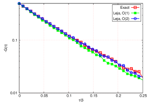
Figure 1: (Color online) Single particle Green’s function $G(\tau)$ of a three-band Hubbard model with $\beta=10$ and $U$ = 2.0 eV computed by the conventional matrix implementation (open squares, exact results) and the Newton-Leja algorithm (filled squares for $O(1)$ level truncation and open circles for $O(2)$ level truncation of the trace).

In the calculation of trace factor, some high-lying eigenstates with negligible contributions can be abandoned in advance to improve the computational efficiency. At low temperature region this truncation approximation is practical, however, at high temperature region it must be used with great care.

We solve the predefined three-band model (see Eq.(16)) at extreme high temperature ($\beta=10$, $T\sim$ 1100 K) and moderate interaction strength ($U$ = 2.0 eV) to explore the influence of truncation approximation to the single particle Green’s function. At first we can obtain the exact solutions by using the conventional matrix algorithm without any truncations. Then we run the simulation again by using the Newton-Leja algorithm with $O(1)$ level (in which only the 4-fold degenerated ground states are retained) and $O(2)$ level (in which not only the 4-fold degenerated ground states but also the 28-fold degenerated first excited states are kept) truncations respectively.

The calculated results are shown in Fig.1. It is apparent that under $O(1)$ level truncation there are significantly systematic deviations between the approximate and exact results, while under $O(2)$ level truncation the deviations can be ignored safely. It has been suggested by Laüchli et al.Lauchli and Werner (2009) that the truncation approximation to the ground state vectors is legitimate just for temperatures which are $\leq 1\%$ of the bandwidth. Therefore in this case the temperature is too high to apply the $O(1)$ level truncation, but the $O(2)$ level truncation is still acceptable. Finally, It should be pointed out that for this model the computational speed with $O(2)$ level truncation is at least twice faster than that of full calculation without any truncations.

IV.2 Accuracy of Newton-Leja algorithm

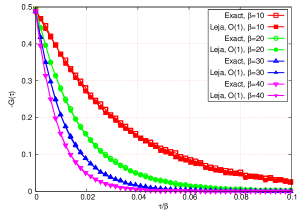
Figure 2: (Color online) Comparison between the single particle Green’s functions of a three-band model computed with the traditional matrix method (open symbols, without any truncations) and those computed with the Newton-Leja algorithm (full symbols, with $O(1)$ level truncation). Upper panel: the calculated single particle Green’s functions at different interaction strengths $U$ and $\beta$ is fixed to 30. Lower panel: the calculated single particle Green’s functions at $U$ = 4.0 eV and different inverse temperatures $\beta$.

Next we try to demonstrate the accuracy of the new approach in a wider parameter range. The top panel of Fig.2 shows the measured single particle Green’s function $G(\tau)$ for $\beta=30$ and different values of the Coulomb interaction strength $U$. Since the model temperature ($T\sim$ 390 K) meets the truncation criterion,Lauchli and Werner (2009), both $O(1)$ and $O(2)$ level truncations are valid. Of course, the $O(2)$ level truncation can give finer results at the cost of performance, so in these simulations we apply the $O(1)$ level truncation merely. In this figure the open symbols were computed with the conventional matrix method without any truncations and used to test the precision of the Newton-Leja algorithm. Not surprisingly, essentially perfect agreement between the two methods is found for all relevant interaction strengths.

The bottom panel of Fig.2 illustrates the calculated results for $U$ = 4.0 eV at different values of inverse temperature $\beta$. The $O(1)$ level truncation is adopted for the Newton-Leja algorithm. The exact solutions obtained by traditional matrix method are shown as a comparison. It is noticed that when the inverse temperature $\beta$ is 10, the deviations between traditional matrix implementation and Newton-Leja algorithm are distinct. The temperature is lower, the smaller the deviation. And for $\beta\geq 20$, the deviations can be considered negligible. In other words, their results become indistinguishable at temperatures which are $\leq 1\%$ of the bandwidth. Nevertheless, the Newton-Leja algorithm with carefully chosen approximations is demonstrated to be controllable, reliable and consistent with original implementations, and can be widely used in standard DMFT calculations.

IV.3 Efficiency of Newton-Leja algorithm

Efficiency is always a major concern for newly developed quantum impurity solver, so it is urgent for us to explore the performance of Newton-Leja algorithm. Based on considerable testing, we found that when the system size is not large enough, the Newton-Leja algorithm is less efficiency than general matrix formulation,Gull et al. (2011a, b) even the Krylov subspace approach.Lauchli and Werner (2009) Whereas, when the system size is large enough, e.g., five-band or bigger model, the situation completely opposite. The Krylov subspace approach outperforms the conventional matrix method and Newton-Leja algorithm is better than the Krylov subspace approach. In this subsection, we try to compare the efficiencies between Newton-Leja algorithm and Krylov subspace approach, and determine the system size for which the former is superior to the latter.

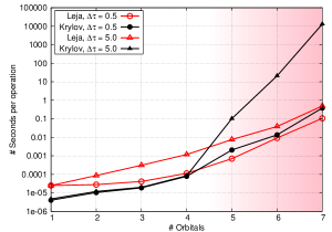
Figure 3: (Color online) Efficiencies (time consumption per evaluation of matrix exponentials $\exp(-\Delta\tau H_{loc})|\nu\rangle$ is used as metric) of the Krylov subspace approach and Newton-Leja algorithm as a function of system size. The local Hamiltonian $H_{loc}$ with rotationally invariant interaction at half-filling is defined in Eq.(16), where $U$ = 4.0 eV and $J/U=0.25$. $\Delta\tau$ = 0.5 and 5.0 for typically short and long time intervals, respectively. The initial vector $|\nu\rangle$ is generated randomly. Both the maximum number of real Leja points for Newton-Leja algorithm $m$ and maximum allowable dimension of Krylov subspace for Krylov approach $p$ are 64. The results obtained by these two algorithms are consistent with each other within the machine precision. In the pink zone, the efficiency of Newton-Leja algorithm is clearly superior to Krylov subspace approach.

Since the key building blocks for both Newton-Leja algorithm and Krylov subspace approach are the calculations of time evolution operators, we just compare their efficiencies by the evaluation of $\exp(-\Delta\tau H_{loc})|\nu\rangle$. Here $|\nu\rangle$ is a randomly generated vector and time step $\Delta\tau$ is set to be 0.5 and 5.0, corresponding to typically short and long time intervals, respectively. The multi-orbital local Hamiltonian $H_{loc}$ is constructed by using Eq.(16), and the interaction strength $U$ is fixed to be 4.0 eV and $J^{\prime}=J=U/4$. Both the maximum allowable dimension for Krylov subspace $p$ and number for real Leja points $m$ are fixed to be 64, which are sufficient to obtain convergent and accurate results.

In order to eliminate the influence of fluctuating measurement data, we repeated every benchmark for 20 times and then evaluated the average time consumption per evaluation of matrix exponentials. The benchmark results for multi-orbital systems with $n=$1, 2, $\cdots$, 7 ($n$ labels the number of bands) are displayed in Fig.3. As can be seen from the figure, when the system size is small or moderate ($n\leq 4$) the Newton-Leja algorithm exhibits worse performance than Krylov subspace approach. However, when increasing the system size continually ($5\leq n\leq 7$, indicated in this figure by pink zone) the Newton-Leja algorithm is the winner. For instance, at $n=5$ and $\Delta\tau=5.0$ the Newton-Leja algorithm is almost ten times faster than the Krylov subspace approach. More impressively, at $n=7$ and $\Delta\tau=5.0$, the Krylov subspace approach is slower than Newton-Leja algorithm about even four orders of magnitude. We note that for short time interval the performances for both implementations are close, but as for $n\geq 5$ the Newton-Leja algorithm still exhibits better performance. According to these benchmarks, it is tentatively suggested that the Newton-Leja algorithm is much more suitable for the systems with five or more orbitals than Krylov subspace approach.

Figure 4: (Color online) Efficiencies (time consumption per evaluation of matrix exponentials $\exp(-\Delta\tau H_{loc})|\nu\rangle$ is used as metric) of the Krylov subspace approach and Newton-Leja algorithm as a function of time interval for the five-band model with rotationally invariant interaction ($U=$ 4.0 eV, $J/U=0.25$). The chemical potential $\mu$ is fixed to fulfill the half-filling condition. Randomly generated vector $|\nu\rangle$ is used as an initial state. The maximum number of real Leja points $m$ is fixed to be 64, while the maximum allowable size of Krylov subspace $p$ is varied from 16 to 64. The convergence criterion for all algorithms are the same. When $\Delta\tau>3.5$, it is very difficult to obtain converged solutions for Krylov subspace approach by current settings.

Next we concentrate our attentions to the five-band model, which plays an important role in the underlying physics of transition metal compounds, and make further benchmarks for our new implementation. The average time consumption per evaluation of matrix exponentials $\exp(-\Delta\tau H_{loc})|\nu\rangle$) is used again as a measurement of efficiency. The model parameters are consistent with previous settings except the time interval $\Delta\tau=0.1\sim 3.5$. The maximum number of real Leja points $m$ is fixed to be 64, while the maximum allowable dimension of Krylov subspace $p$ is varied from 16 to 64. The benchmark results are shown in Fig.4. As is illustrated in this figure, at short ($\Delta\tau<0.8$) and long ($\Delta\tau>1.8$) time intervals, the Newton-Leja algorithm shows better efficiency. It is apparent that when $\Delta\tau>2.0$, actually no decline in efficiency for Newton-Leja algorithm is seen, i.e., the efficiency has nothing to do with the length of time interval. That is because the average degree of Newton interpolation (i.e. number of Leja points used in Newton interpolation) almost remain unchanged. According to our experiences, $m=15\sim 20$ is suitable for most of the five, six, and seven-band models in general parameter ranges. As is mentioned above, provided limiting $m$ and a well defined ellipse containing the eigenvalue spectrum of matrix $-H_{loc}$, a stable interpolant, superlinearly convergent to matrix exponentials $\exp(-\Delta\tau H_{loc})|\nu\rangle$) is guaranteed by the Leja points method (see Eq.(15)).Baglama et al. (1998); Caliari et al. (2004) So we can decrease the maximum number of real Leja points $m$ further to reduce the memory consumption and obtain higher efficiency. As for the Krylov subspace approach, at short time interval region the simulation with smaller Krylov subspace exhibits better performance, while at long time interval region the contrary is indeed true. It is very easy to be understood: at long time interval region, the Krylov subspace algorithm requires larger dimension of subspace to obtain fast convergence speed, and it is hardly to achieve convergence with small dimension of Krylov subspace only when more iterations are done. However, it is impossible to increase the dimension of Krylov subspace infinitely, the oversize of Krylov subspace will deteriorate the performance of Krylov approach quickly.

Table 1: The average computational times per DMFT iteration for typical three-band and five-band Hubbard models solved by hybridization expansion quantum impurity solvers based on Newton-Leja algorithm and Krylov subspace approach respectively. In current simulations, each DMFT iteration took 40000000 Monte Carlo steps per processor, and the results were averaged over 16 processors.

method	three-band model	five-band model
	$U=4.0$ eV and $\beta=20$
Newton-Leja, $m=64$	3.23h	29.07h
Krylov, $p=64$	0.46h	36.80h
	$U=4.0$ eV and $\beta=40$
Newton-Leja, $m=64$	6.12h	67.32h
Krylov, $p=64$	0.78h	399.36h

Finally, two concrete cases are provided to demonstrate the superior performance of Newton-Leja algorithm. Let’s consider typical three-band and five-band Hubbard models respectively. The moderate Coulomb interaction strength $U=4.0$ eV, and inverse temperature $\beta=20\ \text{or}\ 40$ ($T\sim$ 580 K or 290 K) are chosen. These two models are solved separately by hybridization expansion quantum impurity solvers based on Newton-Leja algorithm and Krylov subspace approach with the same computational parameters, and the computational times are gathered and compared with each other. The benchmark results are summarized in table 1. It is confirmed again that for the three-band model Krylov subspace approach is more efficient than Newton-Leja algorithm, yet for the five-band model Newton-Leja algorithm exhibits much better performance, which is consistent with previous benchmark results. Thus by any measure, our new implementation is better than Krylov subspace approach at low temperature and large system size.

V application

In this section, in order to illustrate the usefulness of Newton-Leja algorithm, we used it as a quantum impurity solver in the non-self-consistent LDA+DMFT calculations for representative transition metal oxide SrVO₃. SrVO₃ is a well-known $t^{1}_{2g}e^{0}_{g}$ metal. It is a good test case for LDA+DMFT calculations because it is cubic and nonmagnetic and also the $t_{2g}$ bands are isolated from both $e_{g}$ and oxygen $2p$ bands in the LDA band structure. Numerous theoretical calculations (including LDA+DMFT)Pavarini et al. (2004); Nekrasov et al. (2006); Amadon et al. (2008); Nekrasov et al. (2005) and experimentsEguchi et al. (2006); Yoshida et al. (2005); Sekiyama et al. (2004); Yoshida et al. (2010) have been done on this compound. This is thus an ideal system to benchmark our implementation.

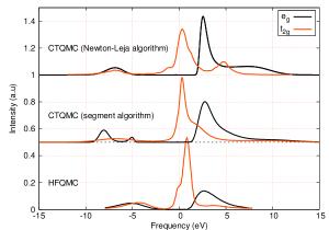
Figure 5: (Color online) The single particle spectral functions for vanadium $3d$ states in SrVO₃ obtained by LDA+DMFT calculations. As for the Newton-Leja algorithm, the rotationally invariant interaction terms are taken into considerations, while for segment algorithmWerner et al. (2006) only the Ising-like density-density interaction terms are treated. The spectral function is obtained from imaginary time Green’s function $G(\tau)$ by using maximum entropy method,Jarrell and Gubernatis (1996) and the calculated results are cross-checked by using recently developed stochastic analytical continuation method.Beach Previous LDA+DMFT results,Amadon et al. (2008) in which traditional HFQMC is used as an impurity solver, are shown in this figure as a comparison.

The LDA+DMFT framework employed in present works has been described in the literatures.Korotin et al. (2008); Trimarchi et al. (2008); Amadon et al. (2008) The ground state calculations have been carried out by using the projector augmented wave (PAW) method with the ABINIT package. The cutoff energy for plane wave expansion is 20 Ha, and the $k$-mesh for Brillouin zone integration is $12\times 12\times 12$. The low-energy effective LDA Hamiltonian is obtained by applying a projection onto maximally localized Wannier function (MLWF) orbitals including all the vanadium $3d$ and oxygen $2p$ orbitals, which is described in details in reference [Amadon et al., 2008]. That would correspond to a $14\times 14$ $p-d$ Hamiltonian which is a minimal modelMossanek et al. (2009) required for a correct description of the electronic structure of SrVO₃.

The LDA+DMFT calculations presented below have been done for the experimental lattice constants ($a_{0}=7.2605$ a.u). All the calculations were preformed in paramagnetic state at the temperature of 1160 K ($\beta=10$). The Coulomb interaction is taken into considerations merely among vanadium $3d$ orbitals. In the present work, we choose $U$ = 4.0 eV and $J$ = 0.65 eV, which are accordance to previous LDA+DMFT calculations.Amadon et al. (2008) We adopt the around mean-field (AMF) scheme proposed in reference [Amadon et al., 2008] to deal with the double counting energy. The effective quantum impurity problem for the DMFT part was solved by two implementations of hybridization expansion CTQMC quantum impurity solver supplemented with recently developed orthogonal polynomial representation algorithm.Boehnke et al. (2011) The former implementation is based on the segment representationWerner et al. (2006) and only the Ising-like density-density interaction terms are treated. The latter implementation is based on the Newton-Leja algorithm, and the local Hamiltonian is with rotationally invariant interactions (see Eq.(16)). The maximum entropy methodJarrell and Gubernatis (1996) was used to perform analytical continuation to obtain the impurity spectral function from imaginary time Green’s function $G(\tau)$ of vanadium $3d$ states. In the present simulations, each LDA+DMFT iteration took 40000000 Monte Carlo steps per process. Since the segment representation hybridization expansion impurity solverWerner et al. (2006) is extreme efficient, it took less 5 hour to finish 30 LDA+DMFT iterations by using a 8-cores Xeon CPU. Though $O(2)$ level approximation is adopted during the simulation, the Newton-Leja algorithm is much more time consumption and took about $12\sim 13$ hours to finish single LDA+DMFT iteration by using 64 cores in a Xeon cluster.

The calculated single particle spectral functions for vanadium $3d$ states in SrVO₃ are shown in Fig.5. The calculated results within density-density interaction are consistent with previous LDA+DMFT simulations.Amadon et al. (2008); Nekrasov et al. (2006, 2005) But the results obtained by classical segment representation and Newton-Leja algorithm display remarkable differences. For examples, the upper and lower Hubbard bands in $t_{2g}$ sub-bands obtained by Newton-Leja algorithm with rotationally invariant interactions are more apparent. And the quasiparticle resonance peak around the Fermi level exhibits clearly shoulder structure, while that shoulder peak is absent in the segment picture (density-density interaction case). Since the vanadium $e_{g}$ sub-bands are isolated from $t_{2g}$ states and located above the Fermi level, so they show roughly similar peak structures for both two implementations of hybridization expansion quantum impurity solvers. Nevertheless, based on our calculated results, it is suggested that the spin-flip and pair-hopping terms in rotationally invariant interactions may play a key role in understanding the subtle electronic structure of SrVO₃ around the Fermi level, which has been ignored by previous theoretical calculations.

VI conclusions

We have presented an alternate implementation of the hybridization expansion quantum impurity solver which makes use of the Newton-Leja interpolation to evaluate the weight of Monte Carlo configurations. The new implementation inherits all the advantages of previously developed Krylov subspace approach with less memory consumption and better convergence control. It shows tremendous growth in computational performance over Krylov subspace approach and conventional matrix implementation at low temperature and large system size, and provides a controlled and efficient way which enables the LDA+DMFT study of transition metal compounds, or even actinide compounds with realistic interactions. To demonstrate the power of the new implementation, we used it as an impurity solver in the LDA+DMFT calculations for typical strongly correlated metal SrVO₃. The obtained impurity spectral function of vanadium $t_{2g}$ states shows apparent distinctions with previous calculated results. It is argued that the full Hund’s exchange may has a big impact on the fine energy spectrum near the Fermi level. The generalization of Newton-Leja algorithm to high performance CUDA-GPU architecture is underway.

Appendix A Leja points

Figure 6: (Color online) The first nine asymmetric real Leja points in [-2:2] interval generated by “Fast Leja Points” algorithm.Baglama et al. (1998) The labels denote the sequences of Leja points.

For the reader’s convenience, here we briefly recall the definition of real Leja points. Sequences of Leja points $\{\xi_{j}\}^{\infty}_{j=0}$ for the compact set $\mathbf{K}$ are defined recursively as follows: if $\xi_{0}$ is an arbitrary fixed point in $\mathbf{K}$, then $\xi_{j}$ are generated recursively in such a way that

$$\prod^{j-1}_{k=0}|\xi_{j}-\xi_{k}|=\max_{\xi\in\mathbf{K}}\prod^{j-1}_{k=0}|\xi-\xi_{k}|,\ j=1,\ 2,\ \cdots.$$ (17)

An efficient algorithm for computing a sequence of real Leja points, the so-called “Fast Leja Points (FLPs)”, has been proposed in reference [Baglama et al., 1998]. In Fig.6 the first nine Leja points in [-2,2] interval are shown as a illustration. The Leja sequences are attractive for interpolation at high-degree, in view of the stability of the corresponding algorithm in the Newton interpolation.Reichel (1990)

Appendix B Newton interpolation

Given a set of $m+1$ data points

$$(x_{0},y_{0}),\ldots,(x_{m},y_{m})$$ (18)

where no two $x_{j}$ are the same, the so-called Newton interpolation polynomial is defined as follows

$$p_{m}(x)=\sum^{m}_{j=0}d_{j}\Omega_{j}(x),$$ (19)

with ${d_{j}}$ the divided differenceCaliari (2007) and the Newton basis polynomial $\Omega_{j}(x)$ defined as

$$\Omega_{j}(x)=\prod^{j-1}_{k=0}(x-x_{k}).$$ (20)

It is apparent that Eq.(12) and Eq.(13) are the matrix forms of Eq.(19) and Eq.(20), respectively. The Newton form is an attractive representation for interpolation polynomials because it can be determined and evaluate rapidly, and, moreover, it is easy to determine $p_{m+1}$ if $p_{m}$ is already known. Because the Leja points are defined recursively, they are attractive to use with the Newton interpolation.

References

- Georges et al. (1996) A. Georges, G. Kotliar, W. Krauth, and M. J. Rozenberg, Rev. Mod. Phys. 68, 13 (1996).
- Kotliar et al. (2006) G. Kotliar, S. Y. Savrasov, K. Haule, V. S. Oudovenko, O. Parcollet, and C. A. Marianetti, Rev. Mod. Phys. 78, 865 (2006).
- Maier et al. (2005) T. Maier, M. Jarrell, T. Pruschke, and M. H. Hettler, Rev. Mod. Phys. 77, 1027 (2005).
- Hirsch and Fye (1986) J. E. Hirsch and R. M. Fye, Phys. Rev. Lett. 56, 2521 (1986).
- Gull et al. (2011a) E. Gull, A. J. Millis, A. I. Lichtenstein, A. N. Rubtsov, M. Troyer, and P. Werner, Rev. Mod. Phys. 83, 349 (2011a).
- Gull et al. (2011b) E. Gull, P. Werner, S. Fuchs, B. Surer, T. Pruschke, and M. Troyer, Comput. Phys. Comm. 182, 1078 (2011b).
- Rubtsov et al. (2005) A. N. Rubtsov, V. V. Savkin, and A. I. Lichtenstein, Phys. Rev. B 72, 035122 (2005).
- Savkin et al. (2005) V. V. Savkin, A. N. Rubtsov, M. I. Katsnelson, and A. I. Lichtenstein, Phys. Rev. Lett. 94, 026402 (2005).
- Werner and Millis (2006) P. Werner and A. J. Millis, Phys. Rev. B 74, 155107 (2006).
- Werner et al. (2006) P. Werner, A. Comanac, L. de’ Medici, M. Troyer, and A. J. Millis, Phys. Rev. Lett. 97, 076405 (2006).
- Haule (2007) K. Haule, Phys. Rev. B 75, 155113 (2007).
- Lauchli and Werner (2009) A. M. Lauchli and P. Werner, Phys. Rev. B 80, 235117 (2009).
- Park and Light (1986) T. J. Park and J. C. Light, J. Chem. Phys. 85, 5870 (1986).
- Hochbruck and Lubich (1997) M. Hochbruck and C. Lubich, SIAM J. Numer. Anal. 34, 1911 (1997).
- Moler and Loan (2003) C. Moler and C. V. Loan, SIAM Rev. 45, 3 (2003).
- Hochbruck and Ostermann (2010) M. Hochbruck and A. Ostermann, Acta Numerica 19, 209 (2010).
- Hochbruck et al. (1998) M. Hochbruck, C. Lubich, and H. Selhofer, SIAM J. Sci. Comp. 19, 1552 (1998).
- Hochbruck and Ostermann (2005) M. Hochbruck and A. Ostermann, Appl. Numer. Math. 53, 323 (2005).
- Sidje (1998) R. B. Sidje, ACM Transactions on Mathematical Software 24, 130 (1998).
- Tal-Ezer (1989) H. Tal-Ezer, Journal of Scientific Computing 4, 25 (1989).
- Bergamaschi et al. (2006) L. Bergamaschi, M. Caliari, A. Martínez, and M. Vianello, in Computational Science - ICCS 2006, Lecture Notes in Comput. Sci., Vol. 3994, edited by V. N. Alexandrov, G. D. van Albada, P. M. A. Sloot, and J. Dongarra (Springer, 2006) pp. 685–692.
- Reichel (1990) L. Reichel, BIT Numerical Mathematics 30, 332 (1990).
- Martínez et al. (2009) A. Martínez, L. Bergamaschi, M. Caliari, and M. Vianello, J. Comput. Appl. Math. 231, 82 (2009).
- Caliari et al. (2004) M. Caliari, M. Vianello, and L. Bergamaschi, J. Comput. Appl. Math. 172, 79 (2004).
- Caliari (2007) M. Caliari, Computing 80, 189 (2007).
- Baglama et al. (1998) J. Baglama, D. Calvetti, and L. Reichel, Electron. Trans. Numer. Anal. 7, 124 (1998).
- Pavarini et al. (2004) E. Pavarini, S. Biermann, A. Poteryaev, A. I. Lichtenstein, A. Georges, and O. K. Andersen, Phys. Rev. Lett. 92, 176403 (2004).
- Nekrasov et al. (2006) I. A. Nekrasov, K. Held, G. Keller, D. E. Kondakov, T. Pruschke, M. Kollar, O. K. Andersen, V. I. Anisimov, and D. Vollhardt, Phys. Rev. B 73, 155112 (2006).
- Amadon et al. (2008) B. Amadon, F. Lechermann, A. Georges, F. Jollet, T. O. Wehling, and A. I. Lichtenstein, Phys. Rev. B 77, 205112 (2008).
- Nekrasov et al. (2005) I. A. Nekrasov, G. Keller, D. E. Kondakov, A. V. Kozhevnikov, T. Pruschke, K. Held, D. Vollhardt, and V. I. Anisimov, Phys. Rev. B 72, 155106 (2005).
- Eguchi et al. (2006) R. Eguchi, T. Kiss, S. Tsuda, T. Shimojima, T. Mizokami, T. Yokoya, A. Chainani, S. Shin, I. H. Inoue, T. Togashi, S. Watanabe, C. Q. Zhang, C. T. Chen, M. Arita, K. Shimada, H. Namatame, and M. Taniguchi, Phys. Rev. Lett. 96, 076402 (2006).
- Yoshida et al. (2005) T. Yoshida, K. Tanaka, H. Yagi, A. Ino, H. Eisaki, A. Fujimori, and Z.-X. Shen, Phys. Rev. Lett. 95, 146404 (2005).
- Sekiyama et al. (2004) A. Sekiyama, H. Fujiwara, S. Imada, S. Suga, H. Eisaki, S. I. Uchida, K. Takegahara, H. Harima, Y. Saitoh, I. A. Nekrasov, G. Keller, D. E. Kondakov, A. V. Kozhevnikov, T. Pruschke, K. Held, D. Vollhardt, and V. I. Anisimov, Phys. Rev. Lett. 93, 156402 (2004).
- Yoshida et al. (2010) T. Yoshida, M. Hashimoto, T. Takizawa, A. Fujimori, M. Kubota, K. Ono, and H. Eisaki, Phys. Rev. B 82, 085119 (2010).
- Jarrell and Gubernatis (1996) M. Jarrell and J. Gubernatis, Phys. Rep. 269, 133 (1996).
- (36) K. S. D. Beach, arXiv:0403055 [cond-mat] .
- Korotin et al. (2008) D. Korotin, A. Kozhevnikov, S. Skornyakov, I. Leonov, N. Binggeli, V. Anisimov, and G. Trimarchi, Eur. Phys. J. B 65, 91 (2008).
- Trimarchi et al. (2008) G. Trimarchi, I. Leonov, N. Binggeli, D. Korotin, and V. I. Anisimov, J. Phys: Condens. Matter 20, 135227 (2008).
- Mossanek et al. (2009) R. J. O. Mossanek, M. Abbate, T. Yoshida, A. Fujimori, Y. Yoshida, N. Shirakawa, H. Eisaki, S. Kohno, P. T. Fonseca, and F. C. Vicentin, Phys. Rev. B 79, 033104 (2009).
- Boehnke et al. (2011) L. Boehnke, H. Hafermann, M. Ferrero, F. Lechermann, and O. Parcollet, Phys. Rev. B 84, 075145 (2011).