Accurate calculation of the solutions to the Thomas-Fermi equations

Abstract

We obtain highly accurate solutions to the Thomas-Fermi equations for atoms and atoms in very strong magnetic fields. We apply the Padé-Hankel method, numerical integration, power series with Padé and Hermite-Padé approximants and Chebyshev polynomials. Both the slope at origin and the location of the right boundary in the magnetic-field case are given with unprecedented accuracy.

1 Introduction

The Thomas-Fermi model is one of the simplest approaches to the study of the potential and charge densities in a variety of systems, like, for example, atoms[1, 2, 3, 4, 5, 6], molecules[7, 4], atoms in strong magnetic fields[8, 9, 10, 6, 11], metals and crystals[12, 13] and dense plasmas[14]. For this reason there has been great interest in the accurate calculation of the solution to the Thomas-Fermi equation[1, 15, 3, 16, 5, 17, 18, 19, 20, 21, 22, 23, 24]. In particular the accurate results obtained by Kobayashi et al[3] by numerical integration are commonly chosen as benchmark data for testing other approaches. The even more accurate results of Rijnierse do not appear to be so well known, probably because they do not appear to have been published and are only quoted in the book by Torrens[5].

The behaviour of the solution to the nonlinear Thomas-Fermi equation depends on the slope at the origin. The critical slope at the origin suitable for neutral atoms is of particular interest and has been estimated by many authors (see, for example, Kobayashi et al[3]). Particularly accurate results for this critical slope were obtained by Amore and Fernández[19, 20] and later by Fernández[21, 22] using the Padé-Hankel method (PHM). Abbasbandy and Bervillier[23] considerably improved this estimate by means of a judicious analytic continuation of the expansion of the solution about the origin and Boyd[24] reported an even more accurate result obtained by means of a rational Chebyshev series. Other authors have also resorted to Padé approximants in order to approximate the solution to the Thomas-Fermi equation[25, 26]. It has been shown that a method due to Majorama is suitable for obtaining a semi-analytical series solution to the Thomas-Fermi equation in terms of only one quadrature[27].

The analytic properties of the solution of the Thomas-Fermi equation under different boundary conditions (in addition to the physically relevant ones) are also of great interest and have been studied by several authors (see, for example, Hille[28, 29] and the references therein).

The purpose of this paper is twofold. First, we want to stress the different behaviour of the solution of the Thomas-Fermi equation for atoms and atoms in strong magnetic fields that was overlooked in a recent application of the PHM[22]. More precisely, in his application of the PHM Fernández[22] assumed the incorrect asymptotic behaviour at infinity suggested by Banerjee et al[8]. However, since the PHM does not take into account the second (outer) boundary condition explicitly Fernández obtained an accurate slope at the origin. The PHM is based on the Riccati-Padé method that was developed to obtain bound states and resonances of separable quantum-mechanical problems[31, 32, 33, 34, 35, 36, 37, 38, 39].

Our second goal is to show that the available computer-algebra software enable one to solve the Thomas-Fermi equations (and, certainly, other nonlinear equations as well) with great accuracy. We want to provide sufficiently accurate solutions that may be used as benchmark data for testing future analytical or numerical methods.

Boyd[24] obtained the most accurate critical slope at the origin of the solution to the Thomas-Fermi equation for neutral atoms by means of rational Chebyshev series. In this paper we try the Chebyshev polynomials on the equation for neutral atoms in very strong magnetic fields.

In Section 2 we outline the expansions of the solution to the Thomas-Fermi equation about origin, at infinity, about poles and zeroes/branch points. Such expansions have already been discussed by other authors and also used as aids for obtaining approximate analytical solutions as well as accurate numerical results[1, 16, 7, 3, 28, 29, 5, 6, 17, 18, 25, 2, 23]. The main purpose of this section is to stress the difference between the Thomas-Fermi equations for isolated atoms and atoms in strong magnetic fields. In section 3 we describe the accurate results obtained by means of the PHM and from straightforward integration of the differential equations. In Sec. 4 we discuss the application of two power series and their Padé and Hermite-Padé approximants to the Thomas-Fermi equation for a neutral atom in a magnetic field. In Sec. 5 we apply Chebyshev polynomials to the same problem and in Sec. 5.2 we consider analytical results based such polynomials of small degree. Finally, in Sec. 6 we draw conclusions.

2 Expansions for the solutions to the Thomas-Fermi equations

In order to facilitate the discussion and to make this paper clearer in this section we summarize the well known expansions of the Thomas-Fermi equations about some characteristic points. As indicated above, such expansions are well known and have been widely used by other authors for several different purposes[1, 16, 7, 3, 28, 29, 5, 6, 17, 18, 25, 2, 23].

In this paper we restrict ourselves to the simplest cases. The first one is the Thomas-Fermi equation for an atom

$$u^{\prime\prime}(x) = \frac{u(x)^{3/2}}{x^{1/2}}$$

$$u(0) = 1$$ (1)

It can be expanded about origin as

$$u=1+ax+\frac{4x^{3/2}}{3}+\frac{2ax^{5/2}}{5}+\frac{x^{3}}{3}+\ldots$$ (2)

where $a=u^{\prime}(0)<0$ is the unknown slope at the origin.

There is a critical slope $u_{0}^{\prime}$ and the behaviour of the solution depends on the relation between $u^{\prime}(0)$ and $u_{0}^{\prime}$. If $u^{\prime}(0)$ $<$ $u_{0}^{\prime}$ the solution vanishes at a movable branch point[29] $x=x_{q}$ around which it behaves as

$$u=bs+b^{3/2}x_{q}^{3/2}\left(\frac{4s^{7/2}}{35}+\frac{2s^{9/2}}{63}+\frac{s^{11/2}}{66}+\ldots\right)$$ (3)

where $s=(x_{q}-x)/x_{q}$ and $b$ is a constant.

If $u^{\prime}(0)$ $>$ $u_{0}^{\prime}$ the solution decreases and reaches a minimum at $x=x_{m}$ about which it behaves as

$$u=a_{0}+(a_{0}x_{m})^{3/2}\left[\frac{s^{2}}{2}+\frac{s^{3}}{12}+\frac{\left(2\sqrt{a_{0}}x_{m}^{3/2}+1\right)s^{4}}{32}+\frac{\left(8\sqrt{a_{0}}x_{m}^{3/2}+5\right)s^{5}}{320}+\ldots\right]$$ (4)

where $s=(x_{m}-x)/x_{m}$ and $a_{0}$ is a positive constant.

After this minimum the solution increases and tends to infinity because of a movable singularity at $x=x_{s}$ about which it behaves as

$$u=\frac{1}{x_{s}^{3}}\left(\frac{400}{s^{4}}-\frac{2000}{9s^{3}}-\frac{2000}{81s^{2}}-\frac{10000}{729s}-\frac{3189895}{177147}+\ldots\right)$$ (5)

where $s=(x_{s}-x)/x_{s}$. Abbasbandy and Bervillier[23] derived an alternative and more detailed expansion in terms of the variable $z=x^{1/2}$ for the function $g(z)=\sqrt{u(z^{2})}$.

It is also well known that $x_{q}\rightarrow\infty$ as $u^{\prime}(0)\rightarrow u_{0}^{\prime}$ from the left and $x_{m},x_{s}\rightarrow\infty$ as $u^{\prime}(0)\rightarrow u_{0}^{\prime}$ from the right. At this limit the solution tends monotonically to zero according to

$$u=\frac{144}{x^{3}}+d\,\,x^{(1-\sqrt{73})/2}+\frac{7\sqrt{73}+67}{29184}d^{2}x^{4-\sqrt{73}}+\ldots$$ (6)

where $d$ is a constant. There have been reasonably successful attempts at matching the expansions (2) and (6) by means of appropriate nonlinear transformations of the independent variable[17, 18].

From a physical point of view the zero at $x=x_{q}$ (see the expansion (3)) is the radio of an atom if

$$-x_{q}u^{\prime}(x_{q})=1-\frac{N}{Z}=q$$ (7)

where $N$ is the number of electrons, $Z$ is the atomic number and $q$ is the degree of ionization (note that $N<Z$). For a neutral atom ($q=0$) the boundary condition $u(x_{0})=u^{\prime}(x_{0})=0$ takes place at $x_{0}=\infty$ as indicated above for the case $u^{\prime}(0)=u_{0}^{\prime}$.

Abbasbandy and Bervillier[23] argued that the PHM applies successfully to this problem because the Hankel condition sends the movable singularity at $x=x_{s}$ to infinity.

The Thomas-Fermi equation for an atom in a strong magnetic field is (Tomishina and Yonei[9] proposed a somewhat more realistic model that we do not discuss here)

$$u^{\prime\prime}(x) = \sqrt{xu(x)}$$

$$u(0) = 1$$ (8)

In this case the expansion about the origin is given by

$$u=1+ax+\frac{4x^{5/2}}{15}+\frac{2ax^{7/2}}{35}+\ldots$$ (9)

where $a=u^{\prime}(0)$. As in the preceding case the behaviour of the solution depends on this slope at the origin that also exhibits a critical value $u_{0}^{\prime}$.

If $u^{\prime}(0)<u_{0}^{\prime}$ the solution vanishes at a movable branch point $x=x_{q}$ according to

$$u=bs+\frac{4\sqrt{b\,x_{1}^{5}}s^{5/2}}{15}-\frac{2\sqrt{b\,x_{1}^{5}}s^{7/2}}{35}+\ldots$$ (10)

where $s=(x_{q}-x)/x_{q}$ and $b$ is a constant.

If $u^{\prime}(0)>u_{0}^{\prime}$ the solution exhibits a minimum at $x=x_{m}$ around which it behaves as

$$u=a_{0}+\frac{\sqrt{a_{0}x_{m}^{5}}}{2}s^{2}-\frac{\sqrt{a_{0}x_{m}^{5}}}{12}s^{3}+\frac{2x_{m}^{5}-\sqrt{a_{0}x_{m}^{5}}}{96}s^{4}-\frac{3\sqrt{a_{0}x_{m}^{5}}+8x_{m}^{5}}{960}s^{5}+\ldots$$ (11)

where $s=(x_{m}-x)/x_{m}$ and $a_{0}$ is a constant.

The main difference between this equation and the preceding one is that in this case the pole is located at infinity. For large values of the coordinate the solution behaves as

$$u=\frac{x^{5}}{400}+c_{0}x^{\left(\sqrt{41}+1\right)/2}+c_{0}^{2}\left(\frac{25\sqrt{41}}{2}+\frac{425}{6}\right)x^{\sqrt{41}-4}+\ldots$$ (12)

where $c_{0}$ is a constant.

When $u^{\prime}(0)=u_{0}^{\prime}$ the solution and its first derivative vanishes at $x=x_{0}$ according to the expansion

$$u=x_{0}^{5}s^{4}\left(\frac{1}{144}-\frac{s}{336}-\frac{s^{2}}{7056}-\frac{s^{3}}{16464}\ldots\right)$$ (13)

where $s=(x_{0}-x)/x_{0}$. The location of the minimum $x_{m}$ approaches $x_{0}$ from below as $u^{\prime}(0)$ approaches $u_{0}^{\prime}$ from above. The zero/branch point $x_{q}$ also approaches $x_{0}$ from below as $u^{\prime}(0)$ approaches $u_{0}^{\prime}$ from below. However, the function is analytic at $x=x_{0}$ when $u^{\prime}(0)=u_{0}^{\prime}$ as shown in Eq. (13). The solution with the critical slope at the origin also tends to infinity as $x\rightarrow\infty$ according to equation (12). According to Banerjee et al[8] the universal solution corresponding to neutral atoms ($N=Z$) satisfies $u(x_{0})=0$ and $u^{\prime}(x_{0})=0$ at $x_{0}=\infty$. Based on this conjecture Fernández[22] applied the PHM and obtained a somewhat more accurate value of $u_{0}^{\prime}$. However Hill et al[11] showed that $x_{0}$ is finite and can be related to $x_{q}$ by means of a perturbation expansion of the form.

$$x_{q}=x_{0}-(24q/x_{0}^{2})^{1/3}+\ldots$$ (14)

which clearly shows that $x_{q}$ approaches $x_{0}$ from below as $q\rightarrow 0$ (and $u^{\prime}(0)\rightarrow u_{0}^{\prime}$ from below). They confirmed this result by numerical integration of Eq. (8).

In the two cases discussed above the PHM yields the correct critical slope at the origin disregarding the second boundary condition. In the first example both $u(x)$ and $u^{\prime}(x)$ vanish as $x\rightarrow\infty$, while in the second example they vanish at a finite value $x_{0}$ of the independent variable. Abbasbandy and Bervillier[23] suggested that the success of the PHM is based on “forcing the localization at infinity of a movable singularity (when it exists)”. They also stated that “if the second boundary is located at infinity, the PHM has a particular significance”. The success of the PHM for the Thomas-Fermi equation (8) shows that the approach is also suitable when the second boundary condition takes place at a finite point. In this case the movable singularity pushed to infinity may be the zero/branch point $x_{q}$ discussed above (Eq. (10)). It was shown that $x_{q}$ approaches $x_{0}$ as $u^{\prime}(0)$ approaches the critical slope but it may jump to infinity when $u^{\prime}(0)=u_{0}^{\prime}$ leaving the solution analytic at $x_{0}$ as discussed above. We cannot prove this conjecture rigorously but we believe that it sounds plausible.

3 PHM and numerical integration

We first review the main points of the PHM. Following Amore and Fernández[19, 20, 21, 22] we choose the new variables $x=t^{2}$ and $v(t)=\sqrt{u(t^{2})}$. The function $v(t)$ can be expanded in a Taylor series

$$v(t)=\sum_{j=0}^{\infty}v_{j}t^{j}$$ (15)

where the coefficients $v_{j}$, $j\geq 4$ depend on $v_{2}=u_{0}^{\prime}/2$.

We construct the Hankel determinants $H_{D}^{d}=\left|v_{i+j+d+1}\right|_{i,j=0,1,\ldots D-1}$ that depend on the unknown slope at the origin $u_{0}^{\prime}$ and obtain sequences of roots $u_{0}^{\prime`}[D,d]$ of $H_{D}^{d}=0$, $D=2,3,\ldots$, ($d=0,1,\ldots$ fixed) that converge towards the critical slope.

We carried out PHM calculations for values of $D$ greater than those used before[22] and also numerical integration based commands built in Mathematica together with the bisection method. We describe the results in what follows.

There are far too many results for the critical slope of the solution to the Thomas-Fermi equation for neutral atoms. Table 1 just shows the most accurate ones. Present PHM result was estimated from sequences of roots of the Hankel determinants with $D\leq 60$ and $d=3$.

The Thomas-Fermi equation for a neutral atom in a strong magnetic field has not been so widely studied. Table 2 shows the available critical slopes at origin. Present PHM result was estimated by comparing results with $D\leq 60$ and $d=1,\,3$. The PHM exhibits a much greater rate of convergence for this problem.

In order to provide benchmark data for testing other approaches in the future we have calculated $u(x)$ and $u^{\prime}(x)$ for Eq. (1) and $u(x)$ for Eq. (8) as accurately as possible using straightforward numerical integration. In principle, we can resort to the analytical behaviour of the solutions described in section 2 in order to bracket the slope at origin $u^{\prime}_{0}$ with any desired accuracy. However, in the present case we have remarkably accurate values of the critical slope at origin obtained by other methods and, therefore, we proceeded in a different way that we describe in what follows.

A sufficiently accurate value of the slope at origin for the Thomas-Fermi equation obtained in this paper is $u^{\prime}(0)=-1.588071022611375312718684508$. We calculated the values of $u(x)$ and $u^{\prime}(x)$ by means of the command NSDolve built in Mathematica with different accuracy choices to test the precision of the numerical results. We tried three sets of parameters:

• Case I: WorkingPrecision=300; PrecisionGoal=20;AccuracyGoal=20;

• Case II: WorkingPrecision=1000; PrecisionGoal=50;AccuracyGoal=50;

• Case III: WorkingPrecision=1000; PrecisionGoal=60;AccuracyGoal=60;

and carried out the numerical integration through the interval $(0,1000)$.

In addition to the straightforward comparison of the results for those three sets it is also necessary to determine the effect of the error due to the approximate choice of $u^{\prime}_{0}$. With this purpose in mind we also carried out the calculations with slightly modified critical slopes:

• $u_{L}^{\prime}(0)=-1.588071022611375312718684509$

• $u_{R}^{\prime}(0)=-1.588071022611375312718684507$

The maximum difference between the values of $u(x)$ obtained with sets I and III at all the chosen points was found to be of order $10^{-14}$, while such difference for sets II and III was $2\times 10^{-20}$. On the other hand, even considering less accurate set I, we found that the maximum difference between values of $u(x)$ calculated with $u_{L}^{\prime}(0)$ and $u_{R}^{\prime}(0)$ was of the order of $10^{-17}$. Thus we conclude that set I yields sufficiently accurate results with the critical slope at origin shown above.

A sample of the results is shown in tables 3, 4 and 5, and a considerably wider range of values is available elsewhere[30]. From the numerical analysis outlined above we are confident that all the digits in those tables are exact.

4 Power-series approaches

4.1 Power-series for the original equation

When $u^{\prime}(0)=u_{0}^{\prime}$ the function is analytic at $x=x_{0}$ and numerical experimentation suggests that the Taylor series (13) converges over the whole domain of interest, even at the left endpoint $x=0$. It is convenient to rescale the coordinate by defining $s=(x_{0}-x)/x_{0}$ so that $x=0$ corresponds to $s=-1$. Therefore we may try to calculate the parameters $u_{0}^{\prime}$ and $x_{0}$ by means of the sequences of partial sums

$$u_{M}(x)=x_{0}^{5}s^{4}\sum_{j=0}^{M}c_{j}s^{j},\,s=\frac{x_{0}-x}{x_{0}}$$ (16)

and the conditions $u_{M}(0)=1$, $u_{M}^{\prime}(0)=u_{0}^{\prime}$. Since the singularity at $s=-1$ ($x=0$) is proportional to $x^{5/2}$ (see Eq. (9)) the coefficients $c_{j}$ decrease as $O(j^{-7/2})$ and the error of the $M-th$ partial sum falls proportionally to $M^{-5/2}$. For example, in this way we obtain $x_{0}\approx 3.06882$ that is correct for five digits versus the actual value $x_{0}\approx 3.068857$. It is remarkable that a power series is able to yield any accuracy at all for a nonlinear, singular boundary value problem.

4.2 Quadratic Padé approximants

Accelerating the convergence by applying ordinary Padé approximations produced no improvement because the function $u$ has a branch point at the left boundary, precisely where we are summing the series to approximate $u^{\prime}(0)$. However, the so-called “Hermite-Padé” or “Shafer” approximation is much more successful.

The quadratic Shafer approximant $u[K/L/M](s)$ is defined to be the solution of the quadratic equation [49, 50, 51, 52]

$$P(s)\,(u[K/L/M])^{2}+Q(s)\,u[K/L/M]\,+\,R(s)=0$$ (17)

where the polynomials $P$, $Q$ and $R$ are of degrees $K$, $L$ and $M$, respectively. These polynomials are chosen so that the power series expansion of $u[K/L/M](s)$ agrees with that of $u(s)$ through the first $N=K+L+M+1$ terms. The constant terms in $P$ and $Q$ can be set arbitrarily to one without loss of generality since these choices do not alter the roots of the equation, so the total number of degrees of freedom is $N=K+L+M+1$. As true for ordinary Padé approximants, the coefficients of the polynomials can be computed by solving a matrix equation and the most accurate approximations are obtained by choosing the polynomials to be of equal degree, so-called “diagonal” approximants. Because the power series begins with $s^{4}$, the method was applied to $\tilde{u}\equiv u(x[s])/(x_{0}^{5}s^{4}$ in the coordinate $s$; the eigenparameter is then estimated from

$$x_{0}\approx\tilde{u}(s=-1)^{-1/5}$$ (18)

The quadratic equation actually yields two approximations:

$$~{}u^{\pm}[K/L/M](s)=\frac{-Q(s)\,\pm\sqrt{Q(s)^{2}-4P(s)\,R(s)}}{2\,P(s)}$$ (19)

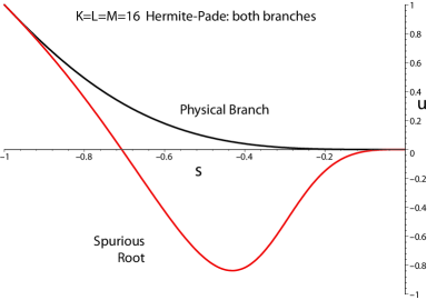
Figure 1: The $K=L=M=16$ Hermite-Padé approximations to $u$ in the coordinate $s=x/x_{0}-1$.

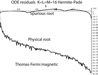
Figure 2: The $K=L=M=16$ Hermite-Padé ODE residuals, that is, the result of substituting the approximation into the Thomas-Fermi differential equation.

as illustrated for $K=L=M=16$ in Fig. 1; the root obtained from applying the minus sign in front of the radical is spuriously negative on much of the interval $s\in[-1,0]$. Substituting $u=x_{0}^{5}s^{4}u^{\pm}[K/L/M]$ into the differential equation yields the “residual function, $\rho^{\pm}=u_{ss}/x_{0}^{2}-\sqrt{x_{0}(s+1)u}$. Plotting the residual functions as in Fig. 2 shows that the “physical” root is the plus sign in (19); the residual function is tiny for the plus root but $O(1)$ for the negative root. One warning is that, like ordinary Padé approximants, Hermite-Padé computations are rather ill-conditioned. We therefore employed Maple so that much of the work was done in exact rational arithmetic, and floating points portions were calculated using 60 decimal digits of precision; we did not investigate ill-conditioning.

The first surprise is that both solution branches of the Hermite-Padé converge to almost the same values as $s\leftrightarrow-1$. We therefore list the errors of the diagonal Shafer approximants for $x_{0}$ from both solutions in Table 6. The table also gives the error of the power series up to order $N$ from whence the Hermite-Padé approximations were obtained. We noticed that the errors of the two branches are roughly equal and opposite; we therefore also list the error in theaverage of the two roots of the quadratic. Each of the roots of the quadratic is a much better approximation than the power series.

In other applications of Hermite-Padé approximations, the roots converge to separate modes, such as one root to the ground state eigenvalue and the other to the first excited state. Here, however, both roots converge to the unique eigenparameter and their average is extraordinarily accurate. We are unaware of another profitable use of averaging in Hermite-Padé approximations.

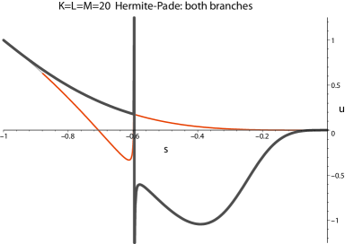
Figure 3: The $K=L=M=20$ Hermite-Padé approximations to $u$ in the coordinate $s=z/x_{0}-1$.

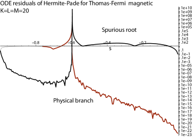
Figure 4: The $K=L=M=20$ Hermite-Padé ODE residuals in the coordinate $s=z/x_{0}-1$.

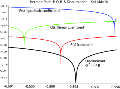
Figure 5: The $K=L=M=20$ Hermite-Padé approximant: Plots of the coefficient polynomials in the quadratics equation $P(f[K/L/M])^{2}+Q\,f[K/L/M]\,+\,R=0$ and also the “discriminant”, $D\equiv Q^{2}-4PR$, which is the argument of the square root in the solutions to the quadratic.

The second surprise is that when $K\geq 17$, the diagonal approximant develops a spurious singularity in the middle of the spatial interval for both branches as illustrated in Fig. 3. Except in a narrow neighborhood of the singularity, the residual function for one branch is very tiny as illustrated in Fig. 4. It has long been known that ordinary Padé approximants may develop similar spurious singularities even at high order and even in spatial regions where the approximants have started to converge; the difficulty is not due to roundoff error, but rather to a near-coincidence of zeros in the numerator and denominator of the rational function which is the Padé approximant [43, 44]. Similarly, the three coefficients of the Hermite-Padé quadratic and also the discriminant, which is the argument of the square root in the approximations, all have nearly coincident zeros as illustrated in Fig. 5. The branches also switch identities at the singularities so that the physical solution is given by the “plus” branch on one side of the singularity and by the “minus” branch on the other side.

This difficulty is not as serious as it seems. Both branches and their average continue to give superb approximations to the eigenparameter $x_{0}$. The ordinary power series converges exponentially fast in the middle of the spatial interval where the Hermite-Padé fails.

The third surprise is that when the order of the approximant is thirty or larger, both roots predict complex-valued $x_{0}$. When $K=L=M=30$, for example, the two branches of the quadratic give errors in $x_{0}$ of $0.199\times 10^{-23}+i0.166\times 10^{-15}$. The imaginary parts cancel when the average is taken, leaving the extraordinarily small and real valued average error of about $0.2\times 10^{-23}$! Thus, in spite of the three surprises, which are also complications, and need for high precision arithmetic at high order, the Hermité-Padé acceleration of the right endpoint Taylor series is very successful.

4.3 Power-series for a modified equation

We can improve the results by removing the singularity through a convenient transformation of the differential equation (8). Instead of the variables discussed above it is more convenient for our aims to choose $x=x_{0}z^{2}$ and $v(z)=\sqrt{u(x_{0}z^{2})}$ so that the differential equation becomes

$$zv(z)v^{\prime\prime}(z)+zv^{\prime}(z)^{2}-v(z)v^{\prime}(z)-2x_{0}^{5/2}z^{4}v(z)=0$$ (20)

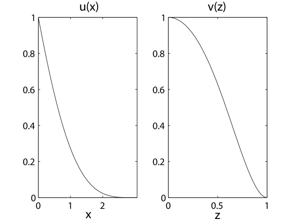
Figure 6: Left: the solution to the Thomas-Fermi problem or strong magnetic field. Right: the transformed unknown $v(z)$ in the rescaled coordinate space $z$.

In this way the domain size $x_{0}$ appears as a sort of eigenparameter $x_{0}$. Fig 6 compares the two functions $u(x)$ and $v(z)$.

We can thus obtain $x_{0}$ and $u_{0}^{\prime}$ from the partial sums

$$v_{M}(z) = x_{0}^{5/2}t^{2}\sum_{j=0}^{M}\tilde{c}_{j}t^{j}$$ (21)

$$= x_{0}^{5/2}t^{2}\left(\frac{1}{3}+\frac{10}{21}t+\frac{149}{588}t^{2}+\ldots\right),\,t=z-1$$

and the equations $v_{M}(0)=1$ and $u_{0}^{\prime}=v_{M}^{\prime\prime}(0)/x_{0}$. Results can be considerably improved by means of Padé approximants $[J,K](t)$. Here we choose diagonal $[M/2,M/2]$ and near-diagonal $[(M-1)/2,(M+1)/2]$ ones because experience and theory suggest that they are usually the most accurate[43, 44, 45]. Tables 7 and 8 show the parameters $u_{0}^{\prime}$ and $x_{0}$ calculated by means of the partial sums (21) and their Padé approximants. The rate of convergence is remarkable for a power-series approach to a nonlinear problem.

5 Chebyshev Pseudospectral Method

We have also written a program that solves the Thomas-Fermi equation using the Chebyshev pseudospectral method and Newton iteration. Because it is so similar to an earlier for the Lane-Emden equation, we omit the details[48].

5.1 Calculations of large order

The solution is approximated in the form

$$v(z)=\sum_{n=0}^{\infty}a_{n}T_{n}(2z-1)$$ (22)

The Chebyshev polynomials can be conveniently evaluated by $T_{n}(z)=\cos(n\,\mbox{arccos}(z))$ or by the usual three term recurrence relation [47].

Newton’s iteration, which was used to solve the system of quadratic equations for the unknowns $(x_{0},a_{0},a_{1},\ldots a_{N})$, requires and initialization or “first guess”. We found that a first guess for $x_{0}\in[2,6]$ combined with the lowest term in the power series, $v\approx x_{0}^{5/2}(z-1)^{2}/3$, suffice to give rapid convergence without underrelaxation.

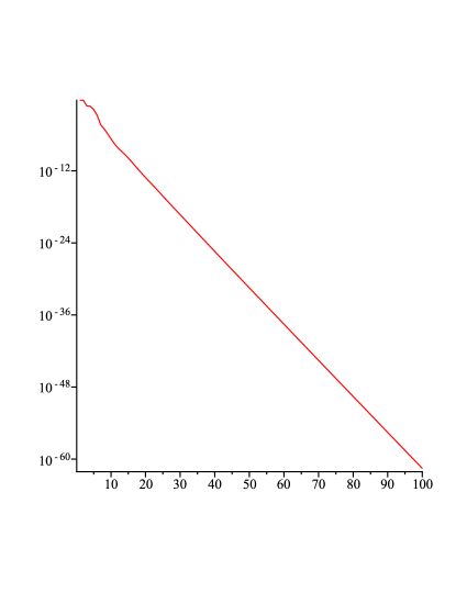
Figure 7: Chebyshev coefficients $a_{n}$ of $v(z)$.

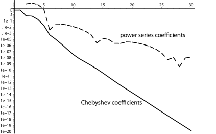
Figure 8: Chebyshev coefficients and power series coefficients of $v(z)$.

The Chebyshev coefficients converge geometrically as illustrated in Fig. 7 with $a_{n}\propto\exp(-n\mu)$ where $\mu$ is between 1.4 and 1.42. All the Chebyshev coefficients larger than $10^{-15}$ listed in Table 9. The Chebyshev series converges much more rapidly than the power series about the right endpoint as illustrated in Fig. 8.

Based on the trends in the Chebyshev calculations, we believe the following results are accurate to all 50 decimal places shown.

$$x_{0}=3.06885718281479942624073100623167158584582595057745$$ (23)

$$u^{\prime}_{0}=-0.93896688764395889305505340187460180383289370739437$$ (24)

5.2 Semi-Analytical Solutions: Chebyshev Polynomial Methods for Small $N$

The most efficient spectral representation is one that incorporates all three boundary conditions into the approximation in a form independent of the spectral coefficients $d_{n}$:

$$v=(z-1)^{2}\,\left\{1+d_{1}[T_{1}(2z-1)+T_{0}]+d_{2}[T_{2}(2z-1)+T_{1}(2z-1)+\ldots\right\}$$ (25)

where we have used the identity $\mbox{sign}(T_{n}(-1))=-\mbox{sign}(T_{n+1}(-1))$ for all $n$. It is convenient, to eliminate fractional powers in the unknowns, to define the new unknown

$$\lambda\equiv 2x_{0}^{5/2}$$ (26)

The pseudospectral method with collocation at the interior points $x_{j}=(1+\cos(\pi j/(N+2))$, $j=1,\ldots(N+1)$ yields a system of coupled polynomial equations, quadratic in the unknowns $(\lambda,d_{1},d_{2},\ldots d_{N})$.

For $N=1$, for example, substitution of $v=(z-1)^{2}\,(1+2d_{1}z)$ into the differential equation yields the residual function

$$resid(z;\lambda,d_{1}) = z\,v\,v^{\prime\prime}+z(v^{\prime})^{2}-\,v\,v^{\prime}-\lambda\,z^{4}\,v$$

$$= 2-2\,\lambda\,z^{7}a_{{0}}+4\,\lambda\,z^{6}a_{{0}}-2\,\lambda\,z^{5}a_{{0}}-6\,z^{2}-64\,z^{3}a_{{0}}+36\,a_{{0}}z^{2}$$

$$- 120\,z^{4}a_{{0}}^{2}+96\,z^{3}a_{{0}}^{2}-24\,a_{{0}}^{2}z^{2}+30\,z^{4}a_{{0}}+48\,z^{5}a_{{0}}^{2}-\lambda\,z^{6}+2\,\lambda\,z^{5}$$

$$- \lambda\,z^{4}+4\,z^{3}-2\,a_{{0}}$$

The coupled system of two equations in two unknowns is the pair of equations $resid(1/4;\lambda,d_{1})=0$ and $resid(3/4;\lambda,d_{1})=0$:

$${\frac{27}{16}}-{\frac{81}{128}}\,d_{{1}}-{\frac{27}{64}}\,{d_{{1}}}^{2}-{\frac{9}{4096}}\,\lambda-{\frac{9}{8192}}\,\lambda\,d_{{1}}=0$$

$${\frac{5}{16}}+{\frac{95}{128}}\,d_{{1}}+{\frac{27}{64}}\,{d_{{1}}}^{2}-{\frac{81}{4096}}\,\lambda-{\frac{243}{8192}}\,\lambda\,d_{{1}} = 0$$ (28)

The resultant of the two equations with elimination of $d_{1}$ is

$${\frac{2705319}{4194304}}+{\frac{1643895}{268435456}}\,\lambda-{\frac{51182361}{68719476736}}\,{\lambda}^{2}+{\frac{1240029}{2199023255552}}\,{\lambda}^{3}=0$$ (29)

This, with substitution of each $\lambda$ root in turn back into one of the residual conditions to determine $d_{1}$, yields the three solutions:

$$\{\lambda=34.33616,d_{1}=1.31544\};\{\lambda=1311.8,d_{1}=-.66653\}$$ (30)

$$\{\lambda=-25.3931,d_{1}=-2.8724\}$$

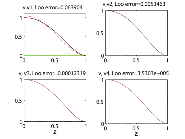
Figure 9: Comparisons of $v(z)$ [solid black] with $N=1$ to $N=4$ Chebsyhev pseudospectral approximations [dashed red]. The green dotted lines, barely visible at the bottom, are the errors.

The first solution is graphed in figure  9; the other two are spurious.

For small $N$, the Maple “solve” command will find all the finite solutions to the system, here $2^{N+1}-1$ in number. In this work, the physical solution was identified as that solution with the eigenparameter $\lambda$ closest to known values found by other means. When no such a priori information is available, a tedious but reliable procedure is to substitute each solution into the differential equation to calculate the residual, and accept the solution with the smallest residual norm. If multiple solutions are suspected, a good strategy is to use each small-$N$solution as a first guess for the Newton pseudospectral code at higher-resolution.

Maple’s system solver is very slow and failed for $N=5$; in contrast, the Newton/collocation program needed only 60 seconds to calculate for $N=100$ in 100 decimal place arithmetic. However, the Maple code that exploits the ”solve” command is much shorter and is given in its entirety in Table 10.

The numerical results, including coefficients up to and including $d_{N}$, are in Table 11 and Fig. 9. Note that only the $N=1$ approximation, obtained by solving a pair of equations for $(\lambda,d_{1})$, is graphically distinguishable from the exact $v(z)$. The success of such low truncations emphasizes the smoothness of the Thomas-Fermi solution in the transformed coordinate $z$ and unknown $u$. it also illustrates that spectral methods can often be used in a semi-analytical mode as described further in [46] and Chapter 20 of [47].

6 Conclusions

We have shown that the PHM converges for two Thomas-Fermi equations that exhibit quite different boundary conditions. In the case of neutral isolated atoms we have $u(x\rightarrow\infty)=0$ and $u^{\prime}(x\rightarrow\infty)=0$ while, on the other hand, $u(x_{0})=0$ and $u^{\prime}(x_{0})=0$ apply to the neutral atoms in very strong magnetic fields. If the success of the PHM depends on the existence of a movable singularity that the approach can push to infinity in the form of a zero of the denominator of the Padé approximant[23], then it seems that two different kinds of singularities are involved in the problems just outlined. According to Abbasbandy and Bervillier[23], in the former case such singular point is precisely the pole $x_{s}$ (see Eq. (5)). However, in the latter case the only candidate appears to be the zero/branch-point $x_{q}$ (see Eq. (10)). Besides, in this case the rate of convergence of the PHM is remarkably larger.

Present PHM calculations of the critical slope at the origin are quite accurate but the generation of analytic Hankel determinants of dimension as large as $D=60$ is time consuming. However, the rate of convergence is commonly so great that one can obtain reasonably accurate results from determinants of relatively small dimension. This feature of the PHM was already exploited by Abbasbandy and Bervillier[23] to estimate the parameters of the conformal mapping used in the analytical continuation of the power series.

We have also shown that nowadays available computer algebra software like Mathematica enable us to obtain the solution to a nonlinear differential equation quite efficiently and accurately by means of suitable built in commands. Such results are shown in tables 4, 4 and 5. However, we found the PHM more convenient for the accurate calculation of the slope at the origin as shown in tables 1 and 2.

In the case of the Thomas-Fermi equation for a neutral atom in a very strong magnetic field we have shown that the power-series expansion about the zero of multiplicity two at $x_{0}$ is a suitable way of obtaining reasonably accurate approximants to the solution over the entire physical interval $0<x<x_{0}$. The results can be slightly improved by means of Padé approximants and considerably improved by means of Hermite-Padé approximations, even when the latter exhibit a singular point or yield complex results at large orders of approximation. If we remove the singularity at origin by means of a suitable transformation both the power series and its Padé approximants lead to remarkably more accurate results.

Finally, we have proved once more that the Chebyshev polynomials are by far the most accurate and efficient way of solving this type of equations. In this application we resorted to another computer-algebra software, Maple.

Table 1: Critical slope at origin for the Thomas-Fermi equation for neutral atoms

Source	$u^{\prime}_{0}$
Ref.[3]	-1.588071
Ref.[5]	-1.5880710
Ref.[22]	-1.588071022611375313
Ref.[23]	-1.5880710226113753127189$\pm 7\times 10^{-22}$
Ref.[24]	-1.5880710226113753127186845
Present (integration)	-1.588071022611375312718684
Present (PHM)	-1.588071022611375312718684508

Table 2: Critical slope at origin for the Thomas-Fermi equation for neutral atoms in strong magnetic fields

Source	$u^{\prime}_{0}$
Ref.[8]	-0.93896594
Ref.[11]	-0.938966887644
Ref.[22]	-0.93896688764395889306
Present (PHM)	-0.9389668876439588930550534018746018038328937073944

Table 3: Solution to the Thomas-Fermi equation for neutral atoms

$x$	$u(x)$
0	1.
10	0.024314292988681
20	0.0057849411915669
30	0.0022558366162029
40	0.0011136356388334
50	0.0006322547829849
60	0.00039391136668542
70	0.00026226529981201
80	0.00018354575974071
90	0.00013354582895373
100	0.00010024256813941
110	0.000077192183914122
120	0.000060724454048042
130	0.000048642170611589
140	0.000039574139448193
150	0.000032633964446257
160	0.000027231036946158
170	0.000022961351007399
180	0.000019542101672266
190	0.000016771248041131
200	0.000014501803496946
210	0.00001262507868731
220	0.000011059514500269
230	9.7430900509356e-6
240	8.6280669794388e-6
250	7.6772907646176e-6
260	6.8615483807441e-6
270	6.1576544141983e-6
280	5.5470471166532e-6
290	5.0147463894448e-6
300	4.548571953617e-6
310	4.1385507917383e-6
320	3.7764638007387e-6
330	3.4554958931053e-6
340	3.1699637128939e-6
350	2.9151021105849e-6
360	2.6868954790918e-6
370	2.4819436135582e-6
380	2.2973543393218e-6
390	2.1306570419327e-6
400	1.9797326281136e-6
410	1.842756484985e-6
420	1.7181517839461e-6
430	1.6045510644226e-6
440	1.5007644808624e-6
450	1.4057534397658e-6
460	1.3186086183364e-6
470	1.2385315617813e-6
480	1.1648192165876e-6
490	1.0968508828835e-6
500	1.034077168203e-6
510	9.7601060362214e-7
520	9.2221764589762e-7
530	8.7231183937678e-7
540	8.2594795176694e-7
550	7.828169303947e-7
560	7.4264155197267e-7
570	7.0517266036529e-7
580	6.7018590439059e-7
590	6.3747890208209e-7
600	6.0686876967458e-7
610	5.7818996335412e-7
620	5.5129238991189e-7
630	5.2603974917333e-7
640	5.0230807668597e-7
650	4.7998445984162e-7
660	4.5896590454401e-7
670	4.3915833284169e-7
680	4.2047569473637e-7
690	4.0283917973564e-7
700	3.861765157183e-7
710	3.7042134437901e-7
720	3.5551266396608e-7
730	3.4139433126073e-7
740	3.2801461580316e-7
750	3.1532580027683e-7
760	3.032838217405e-7
770	2.918479490687e-7
780	2.8098049253898e-7
790	2.7064654200495e-7
800	2.6081373052692e-7
810	2.5145202070801e-7
820	2.4253351131026e-7
830	2.3403226200994e-7
840	2.2592413439939e-7
850	2.1818664755992e-7
860	2.1079884671993e-7
870	2.0374118367901e-7
880	1.9699540782507e-7
890	1.9054446669994e-7
900	1.8437241518212e-7
910	1.7846433245545e-7
920	1.7280624602028e-7
930	1.6738506208215e-7
940	1.6218850172182e-7
950	1.5720504231184e-7
960	1.5242386369939e-7
970	1.4783479872324e-7
980	1.4342828767613e-7
990	1.3919533636191e-7
1000	1.3512747743129e-7

Table 4: First derivative of the Solution to the Thomas-Fermi equation for neutral atoms

$x$	$u^{\prime}(x)$
0	-1.5880710226114
10	-0.0046028818712693
20	-0.00064725433277769
30	-0.00018067000647699
40	-0.000069668028540326
50	-0.000032498902048259
60	-0.0000171977000831
70	-9.9565333930524e-6
80	-6.1661955287641e-6
90	-4.0244737037667e-6
100	-2.7393510686783e-6
110	-1.9299022690995e-6
120	-1.3992583170223e-6
130	-1.0395157118193e-6
140	-7.8856447021428e-7
150	-6.0913994786089e-7
160	-4.7807415548727e-7
170	-3.8051134288369e-7
180	-3.0666432312939e-7
190	-2.4992901331678e-7
200	-2.0575323164753e-7
210	-1.7093867858999e-7
220	-1.4319925950792e-7
230	-1.2087522043829e-7
240	-1.0274430764511e-7
250	-8.7894679831444e-8
260	-7.5637914908074e-8
270	-6.544852781645e-8
280	-5.6921313455898e-8
290	-4.9740860705699e-8
300	-4.3659496185299e-8
310	-3.8481144114006e-8
320	-3.4049389482697e-8
330	-3.0238562022714e-8
340	-2.6947014494947e-8
350	-2.4092011004349e-8
360	-2.1605807799308e-8
370	-1.9432625152504e-8
380	-1.7526290677749e-8
390	-1.5848392577797e-8
400	-1.4366823059949e-8
410	-1.3054622396184e-8
420	-1.1889056199565e-8
430	-1.0850874763838e-8
440	-9.9237153936954e-9
450	-9.0936176860656e-9
460	-8.3486285238475e-9
470	-7.6784786982998e-9
480	-7.0743170080134e-9
490	-6.5284906994362e-9
500	-6.0343634424472e-9
510	-5.5861638415855e-9
520	-5.1788588934186e-9
530	-4.8080479060999e-9
540	-4.4698732683358e-9
550	-4.160945144665e-9
560	-3.878277722421e-9
570	-3.6192350738087e-9
580	-3.3814850478544e-9
590	-3.1629598899054e-9
600	-2.9618225150474e-9
610	-2.7764375473743e-9
620	-2.6053463881518e-9
630	-2.4472456993964e-9
640	-2.3009687906329e-9
650	-2.1654694798767e-9
660	-2.0398080686052e-9
670	-1.9231391273669e-9
680	-1.8147008358921e-9
690	-1.7138056608835e-9
700	-1.6198321874803e-9
710	-1.5322179478635e-9
720	-1.4504531135232e-9
730	-1.3740749371114e-9
740	-1.3026628461653e-9
750	-1.2358341048206e-9
760	-1.1732399713605e-9
770	-1.1145622894042e-9
780	-1.0595104590168e-9
790	-1.0078187412534e-9
800	-9.59243855836e-10
810	-9.135628369537e-10
820	-8.7057111672569e-10
830	-8.3008080977438e-10
840	-7.9191917572404e-10
850	-7.5592723934792e-10
860	-7.2195855060047e-10
870	-6.8987806894922e-10
880	-6.5956115831007e-10
890	-6.3089268053242e-10
900	-6.0376617681006e-10
910	-5.7808312764064e-10
920	-5.5375228304499e-10
930	-5.3068905571025e-10
940	-5.0881497055441e-10
950	-4.8805716494193e-10
960	-4.6834793442266e-10
970	-4.4962431943178e-10
980	-4.3182772888659e-10
990	-4.1490359705517e-10
1000	-3.9880107046013e-10

Table 5: Solution to the Thomas-Fermi equation for neutral atoms in strong magnetic fields

$x$	$u(x)$
0.	1.
0.1	0.7170931035374508
0.2	0.6124516884444692
0.3	0.5381961080581211
0.4	0.479844885457407
0.5	0.4317097837447453
0.6	0.3908409649565394
0.7	0.3554696879373627
0.8	0.3244342852150042
0.9	0.2969222776883283
1.	0.2723385646065789
1.1	0.2502315742397729
1.2	0.2302489290264509
1.3	0.2121093520054812
1.4	0.1955840735228681
1.5	0.1804840769457186
1.6	0.1666510831170969
1.7	0.1539510127378397
1.8	0.1422691401494945
1.9	0.1315064314341758
2.	0.1215767304319089
2.1	0.1124045638520199
2.2	0.1039234063491158
2.3	0.09607429270074567
2.4	0.08880469561358382
2.5	0.0820676094016386
2.6	0.07582079507183087
2.7	0.07002615329387998
2.8	0.06464919967550395
2.9	0.05965862260930963
3.	0.05502590831205111
3.1	0.05072502095749841
3.2	0.04673212830182475
3.3	0.04302536512062993
3.4	0.0395846282664133
3.5	0.03639139832082583
3.6	0.03342858373515079
3.7	0.0306803840826662
3.8	0.02813216963071108
3.9	0.02577037491068775
4.	0.02358240434538228
4.1	0.02155654830361774
4.2	0.01968190820681658
4.3	0.01794832952175207
4.4	0.0163463416473783
4.5	0.01486710384803269
4.6	0.01350235650595824
4.7	0.0122443770673297
4.8	0.01108594014126138
4.9	0.01002028128341276
5.	0.00904106405704823
5.1	0.008142350016579636
5.2	0.007318571303218951
5.3	0.006564505580616747
5.4	0.005875253071267334
5.5	0.005246215482854354
5.6	0.004673076638280921
5.7	0.004151784644449602
5.8	0.003678535453408486
5.9	0.003249757685661876
6.	0.002862098599594876

Table 6: Errors in Eigenlength $x_{0}$ for the magnetic case, obtained from right endpoint power series and Hermite-Padé approximation for $u(x)$

$K$ ($=L=M$)	$N$	Taylor series	first root	second root	average of roots
2	7	0.0039	0.0023	0.044	0.023
5	16	0.00076	0.00093	0.000052	0.00043
10	31	$0.174\times 10^{-3}$	$0.265\times 10^{-6}$	$0.32\times 10^{-6}$	$0.31\times 10^{-7}$
15	46	$0.69\times 10^{-4}$	$0.11\times 10^{-8}$	$0.11\times 10^{-8}$	$0.32\times 10^{-11}$
20	61	$0.35\times 10^{-4}$	$0.15\times 10^{-11}$	$0.15\times 10^{-11}$	$0.45\times 10^{-15}$
25	76	$0.21\times 10^{-4}$	$0.11\times 10^{-12}$	$0.11\times 10^{-12}$	$0.39\times 10^{-18}$

Table 7: $v$-power series approximation of initial slope $u^{\prime}_{0}$; correct digits in boldface

$M$	Method	$u^{\prime}_{0}$	Number of correct digits
10	power series	-0.9364	2
	Padé	-0.9327	2
20	power series	-0.93879	3
	Padé	-0.9389645	5
40	power series	-0.938966834	7
	Padé	-0.93896688760	9
60	power series	-0.938966887635	10
	Padé	-0.9389668876439554	14
80	power series	-0.9389668876439574	14
	Padé	-0.9389668876439588927	17
—	PHM[22]	-0.93896688764395889306	20

Table 8: Eigenparameter $x_{0}$ approximations from the $v$-power series

$M$	Method	$x_{0}$
10	power series	3.068806
	Padé	3.06877
20	power series	3.0688560
	Padé	3.068857176
40	power series	3.06885718271
	Padé	3.068857182814799451
60	power series	3.0688571828147917
	Padé	3.06885718281479942624073139
80	power series	3.0688571828147994255
	Padé	3.068857182814799426240731006231672626130

Table 9: Chebyshev coefficients of the solution to the magnetic case of the Thomas-Fermi equation

degree $n$	$a_{n}$
0	$5.48135788388634344\times 10{-01}$
1	$-5.58881613523477153\times 10{-01}$
2	$-6.42705283349619230\times 10{-02}$
3	$5.70880541499120995\times 10{-02}$
4	$1.61861107728602653\times 10{-02}$
5	$1.78344934649533460\times 10{-03}$
6	$-4.97638953814069498\times 10{-05}$
7	$9.88568187276911699\times 10{-06}$
8	$-1.57314041941070364\times 10{-06}$
9	$2.17031601079801803\times 10{-07}$
10	$-3.17277060187282838\times 10{-08}$
11	$6.73733273124207577\times 10{-09}$
12	$-1.91849909540107163\times 10{-09}$
13	$5.43530178894964329\times 10{-10}$
14	$-1.37539658139417754\times 10{-10}$
15	$3.12411846416475022\times 10{-11}$
16	$-6.65185565734159168\times 10{-12}$
17	$1.41167490452475800\times 10{-12}$
18	$-3.15485896233555226\times 10{-13}$
19	$7.52433060541288362\times 10{-14}$
20	$-1.85848288796828985\times 10{-14}$
21	$4.57976772880843444\times 10{-15}$
22	$-1.10484891112084068\times 10{-15}$

Table 10: Maple Code to Compute a Chebyshev Pseudospectral Approximation for Small $N$

restart; with(orthopoly); N:=4; # Define approximation in next 2 lines;

vv:=1; for n from 1 to N do vv:=vv + d[n]*(T(n,2*x-1)+T(n-1,2*x-1)); od:

v:= (x-1)*(x-1)*vv; # derivatives of v; vx:=diff(v,x); vxx:=diff(v,x,x);

resid:= x*v*vxx + x*vx*vx -v*vx - lambda* x**4 *v; # ODE residual;

ta[0]:=evalf( Pi*(0+1)/(N+2) ); xa[0]:=evalf((cos(ta[0])+1)/2); # Chebyshev grid points ”xa”;

resida[0]:= evalf(subs(x=xa[0],resid));

varset:= lambda; eqset:= resida[0]; # initialize set of unknowns & the set of pointwise residuals;

for j from 1 to N do ta[j]:= evalf( Pi*(j+1)/(N+2) );

xa[j]:= evalf( (cos(ta[j] ) + 1)/2 ); resida[j]:= evalf(subs(x=xa[j],resid)); # array of ODE residuals ;

varset:= varset union d[j]; eqset:= eqset union resida[j]; # update variable & equation sets; od:

solutionvector:=solve(eqset,varset); assign(solutionvector[1]); # solve the polynomial system;

# {resida[j]=0, j=0, …, N} in unknowns {$\lambda,d_{1},\ldots d_{N}$} ;

xi:= evalf( (lambda/2)**(2/5) ); sigma:= evalf( subs(x=0,diff(v,x,x)/xi) );

Table 11: Results and Errors from Low Order Collocation

Name	$N=1$	$N=2$	$N=3$	$N=4$	Exact
$x_{0}$	3.11809	3.07417	3.0687055	3.068876456	3.0688571
$x_{0}$ error	0.049	0.0053	-0.00015	$0.19274\times 10{-4}$	—
$u^{\prime}_{0}$	-2.73	-.281	-.89047	-.9237607	-0.9389669
$u^{\prime}_{0}$ error	-1.79	0.66	0.048	0.015	—
$d_{1}$	1.315	1.8211	1.8837159	1.882043824	1.8825071389
$d_{2}$		.29256	.34172159	.3402298497	.34061038
$d_{3}$			0.027764	0.0266875	.0269894965
$d_{4}$				-0.000662	-.0004613479537

References

- [1] E. B. Baker, The application of the Fermi-Thomas statistical model to the calculation of potential distribution in positive ions, Phys. Rev. 36 (1930) 630-646.
- [2] C. A. Coulson, N. H. March, Momenta in atoms using the Thomas-Fermi method, Proc. Phys. Soc. A63 (1950) 367-374.
- [3] S. Kobayashi, T. Matsukuma, S. Nagai, K. Umeda, Accurate value of the initial slope of the ordinary TF function, J. Phys. Soc. Japan 10 (1955) 759-762.
- [4] N. H. March, The Thomas-Fermi approximation in quantum mechanics, Adv. Phys. 6 (1957) 1-101.
- [5] I. M. Torrens, Interatomic Potentials, Academic, New York, 1972.
- [6] N. H. March, Origins-The Thomas-Fermi theory, in: S. Lundqvist and N. H. March (Ed.), Theory of the inhomogeneous electron gas, Vol. Plenum Press, New York, London, 1983.
- [7] N. H. March, Thomas-Fermi fields for molecules with tetrahedral and octahedral symmetry, Proc. Camb. Phil. Soc. 48 (1952) 665-682.
- [8] B. Banerjee, D. H. Constantinescu, P. Rehák, Thomas-Fermi and Thomas-Fermi-Dirac calculations for atoms in a very strong magnetic field, Phys. Rev. D 10 (1974) 2384-2395.
- [9] Y. Tomishina, K. Yonei, Thomas-Fermi theory for atoms in a strong magnetic field, Prog. Theor. Phys. 59 (1978) 683-696.
- [10] N. H. March, Y. Tomishina, Behaviour of positive ions in extremely strong magnetic fields, Phys. Rev. D 19 (1979) 449-450.
- [11] S. H. Hill, P. J. Grout, N. H. March, Chemical potential and total energy of heavy positive atoms in extremely strong magnetic fields, near the weak ionisation limit, J. Phys. B 16 (1983) 2301-2307.
- [12] J. C. Slater, H. M. Krutter, The Thomas-Fermi Method for Metals, Phys. Rev. 47 (1935) 559-568.
- [13] K. Umeda, Y. Tomishina, On the influence of the packing on the atomic scattering factor based on the Thomas-Fermi theory, J. Phys. Soc. Jap. 10 (1955) 753-758.
- [14] R. Ying, G. Kalman, Thomas-Fermi model for dense plasmas, Physical Review A 40 (1989) 3927-3950.
- [15] V. Bush, S. H. Caldwell, Thomas-Fermi equation solution by the differential analyzer, Phys. Rev. 38 (1931) 1898-1902.
- [16] R. P. Feynman, N. Metropolis, E. Teller, Equations of state of elements based on the generalized Fermi-Thomas Theory, Physical Review 75 (1949)
- [17] G. I. Plindov, S. K. Pogrebnya, The analytical solution of the Thomas-Fermi equation for a neutral atom, J. Phys. B 20 (1987) L547-L550.
- [18] F. M. Fernández, J. F. Ogilvie, Approximate solutions to the Thomas-Fermi equation, Phys. Rev. A 42 (1990) 149-154.
- [19] P. Amore, F. M. Fernández, Rational Approximation for Two-Point Boundary value problems, arXiv:0705.3862
- [20] P. Amore, F. M. Fernández, Rational approximation to the solutions of two-point boundary value problems, Acta Polytech. 51 (2011) 9-13.
- [21] F. M. Fernández, Comment on: ”Series solution to the Thomas-Fermi equation” [Phys. Lett. A 365 (2007) 111], Phys. Lett. A 372 (2008) 5258-5260.
- [22] F. M. Fernández, Rational approximation to the Thomas-Fermi equations, Appl. Math. Comput. 207 (2011) 6433-6436.
- [23] S. Abbasbandy, C. Bervillier, Analytic continuation of Taylor series and the boundary value problems of some nonlinear ordinary differential equations, Appl. Math. Comput. 218 (2011) 2178-2199.
- [24] J. P. Boyd, Rational Chebyshev Series for the Thomas-Fermi Function: Endpoint Singularities and Spectral Methods, J. Comp. Appl. Math. (2012) in the press.
- [25] K. Tu, Analytic solution to the Thomas-Fermi and Thomas-Fermi-Dirac-Weizsäcker equations, J. Math. Phys. 32 (1991) 2250-2253.
- [26] L. N. Epele, H. Fanchiotti, C. A. García Canal, J. A. Ponciano, Padé approximant approach to the Thomas-Fermi problem, Phys. Rev. A 60 (1999) 280-283.
- [27] S. Esposito, Majorana solution of the Thomas-Fermi equation, Am. J. Phys. 70 (2002) 852-856.
- [28] E. Hille, On the Thomas-Fermi equation, Proc. Natl. Acad. Sci. USA 62 (1969) 7-10.
- [29] E. Hille, Some aspects of the Thomas-Fermi equation, J. Anal. Math. 23 (1970) 147-170.
- [30] P. Amore, J. P. Boyd, and F. M. Fernández, Accurate calculation of the solutions to the Thomas-Fermi equations, arXiv:1205.1704v1 [quant-ph].
- [31] F. M. Fernández, Q. Ma, R. H. Tipping, Tight upper and lower bounds for energy eigenvalues of the Schrödinger equation, Phys. Rev. A 39 (1989) 1605-1609.
- [32] F. M. Fernández, Strong Coupling Expansion for Anharmonic Oscillators and Perturbed Coulomb Potentials, Phys. Lett. A 166 (1992) 173-176.
- [33] F. M. Fernández, R. Guardiola, Accurate Eigenvalues and Eigenfunctions for Quantum-Mechanical Anharmonic Oscillators, J. Phys. A 26 (1993) 7169-7180.
- [34] F. M. Fernández, Direct Calculation of Accurate Siegert Eigenvalues, J. Phys. A 28 (1995) 4043-4051.
- [35] F. M. Fernández, Alternative Treatment of Separable Quantum-mechanical Models: the Hydrogen Molecular Ion, J. Chem. Phys. 103 (1995) 6581-6585.
- [36] F. M. Fernández, Resonances for a Perturbed Coulomb Potential, Phys. Lett. A 203 (1995) 275-278.
- [37] F. M. Fernández, Quantization Condition for Bound and Quasibound States, J. Phys. A 29 (1996) 3167-3177.
- [38] F. M. Fernández, Direct Calculation of Stark Resonances in Hydrogen, Phys. Rev. A 54 (1996) 1206-1209.
- [39] F. M. Fernández, Tunnel Resonances for One-Dimensional Barriers, Chem. Phys. Lett 281 (1997) 337-342.
- [40] B. Boisseau, P. Forgács, H. Giacomini, An analytical approximation scheme to two-point boundary value problems of ordinary differential equations, J. Phys. A 40 (2007) F215-F221.
- [41] C. Bervillier, Conformal mappings versus other power series methods for solving ordinary differential equations: illustration on anharmonic oscillators., J. Phys. A 42 (2009) 485202 (485217pp).
- [42] C. Bervillier, B. Boisseau, H. Giacomini, Analytical approximation schemes for solving exact renormalization group equations. II Conformal mappings, Nucl. Phys. B 801 (2008) 296-315.
- [43] G. A. Baker Jr (Eds.), Padé Approximants, Academic Press, New York, 1965, Vol. 1.
- [44] G. A. Baker Jr, Essentials of Padé Approximants, Academic Press, New York, 1975.
- [45] C. M. Bender, S. A. Orszag, Advanced mathematical methods for scientists and engineers, McGraw-Hill, New York, 1978.
- [46] J. P. Boyd, Chebyshev and Legendre spectral methods in algebraic manipulation languages, J. Symb. Comp. 16 (1993) 377-399.
- [47] J. P. Boyd, Chebyshev and Fourier Spectral Methods, Dover, Mineola, 2001.
- [48] J. P. Boyd, Chebyshev SpectralMethods and the Lane-Emden Problem, Numer. Math. Theor. Meth. Appl. 4 (2011) 142-157
- [49] A. V. Sergeev, D. A. Goodson, Summation of asymptotic expansions of multiple-valued functions using algebraic approximants: Application to anharmonic oscillators, J. Phys. A 31 (1998) 4301-4317.
- [50] R. E. Shafer, On quadratic approximation, SIAM J. Num. Anal. 11 (1974) 447-460.
- [51] J. P. Boyd, A. Natarov, Shafer (Hermite-Padé) approximants for functions with exponentially small imaginary part with application to equatorial waves with critical latitude, Appl. Math. Comput. 126 (2002) 109-117.
- [52] J. P. Boyd, The Devil’s Invention: Asymptotics, Superasymptotics and Hyperasymptotics, Acta Applicandae Mathematicae 56 (1999) 1-98.