New spectral relations between products and powers of isotropic random matrices

Abstract

We show that the limiting eigenvalue density of the product of $n$ identically distributed random matrices from an isotropic unitary ensemble (IUE) is equal to the eigenvalue density of $n$-th power of a single matrix from this ensemble, in the limit when the size of the matrix tends to infinity. Using this observation one can derive the limiting density of the product of $n$ independent identically distributed non-hermitian matrices with unitary invariant measures. In this paper we discuss two examples: the product of $n$ Girko-Ginibre matrices and the product of $n$ truncated unitary matrices. We also provide an evidence that the result holds also for isotropic orthogonal ensembles (IOE).

PACS: 02.50.Cw (Probability theory), 02.70.Uu (Applications of Monte Carlo methods)
Keywords: isotropic random matrices, free probability;

Introduction

Free probability theory is a fusion of non-commutative probability theory and the concept of free independence. Since 1991, when the link between the free probability theory and random matrix theory was established vdn , several new results have been proven in an easy and powerful way in the limit of infinitely large random matrices hp ; agz ; ns . In this note we demonstrate a simple albeit quite counterintuitive result that the spectral density of the product of $n$ free, identically distributed random matrices from an isotropic unitary ensemble (IUE) is equal to the spectral density of the $n$-th power of a single matrix from this ensemble in the limit of infinite matrix size. The proof is based on the multiplicative properties of the S-transform and the Haagerup-Larsen theorem hl .

The motivation for the present work comes from the observation made in bjw ; agt1 ; agt2 that the eigenvalue density of $n$ independent Girko-Ginibre g1 ; g2 matrices is identical to the eigenvalue density of the $n$-th power of a single Girko-Ginibre matrix in the limit of infinite size. This observation leads to the question whether this is a feature of only this particular class of matrices or if there exists a larger class of matrices that have this property. In the present paper we show that there is indeed a larger class of matrices sharing this property - a class of random isotropic matrices. We begin with defining isotropic matrices. Then we present the main result in detail and its derivation. Finally we outline a few sample applications, related to the recent interest in the literature. In particular we apply our result to the product of Ginibre-Girko matrices and rederive the density known from bjw ; agt1 ; agt2 . We also consider classes of truncated unitary and orthogonal matrices and compare our predictions to Monte Carlo simulations, which allow us to identify finite size corrections. We conclude the paper with a short summary.

Isotropic random matrices

It is convenient to introduce the concept of isotropic random matrices in analogy to isotropic complex random variables $z$ that have a circularly symmetric probability distribution depending only on the module $|z|$. Using polar decomposition, one can write $z=re^{i\phi}$ where $r$ is a real non-negative random variable and $\phi$ is a random variable (phase) with a uniform distribution on $[0,2\pi)$. Isotropic random matrices are defined by a straightforward generalization of isotropic complex random variables. A square $N\times N$ matrix $x$ is said to be isotropic random matrix if it has a polar decomposition $x=hu$ in which $h$ is a positive semi-definite Hermitian random matrix and $u$ is a unitary random matrix independent of $h$ and distributed on the unitary group $U(N)$ with the Haar measure. In short, $u$ is a Haar unitary matrix. The random matrix $h$ plays the role of the radial part of $x$. Such random matrices form an ensemble of isotropic unitary matices (IUE). An example is an ensemble generated by the partition function fz ; fsz :

$$Z=\int Dx\ e^{-N{\rm Tr}V(x^{\dagger}x)}$$ (1)

where $Dx=\prod_{ij}d({\rm Re}x_{ij})d({\rm Im}x_{ij})$ is a flat measure, and $V(a)$ is a polynomial in $a$. Another natural class of IUE matrices are matrices of the form $x=vdu$ where $d$ is an $N\times N$ diagonal matrix having real positive random eigenvalues with the given probability distribution and $v$ and $u$ are two independent Haar unitary matrices on the unitary group $U(N)$. By analogy one can also consider isotropic orthogonal ensemble (IOE) given by the decomposition $x=so$ with $s$ being a positive semidefinite real symmetric matrix and $o$ being a Haar orthogonal matrix. In this case, when one considers an ensemble given by a partition function like that given above, one has to replace $x$ by a real matrix.

In mathematical literature, isotropic matrices for $N\rightarrow\infty$ are called $R$-diagonal ns2 . In this note we prefer to call them isotropic (or IUE, IOE) in the large $N$ limit. IUE matrices have an eigenvalue distribution independent of the polar angle on the complex plane. In the limit when the matrix size $N\rightarrow\infty$ one can find an explicit relation between the eigenvalue density of the matrix $h^{2}$ and of the matrix $x$ hl ; fz ; fsz ; gkz . We briefly recall this relation below. Let us mention that the angular independence of the eigenvalue density does not imply that the matrix is isotropic. For example a block diagonal matrix of the form:

$$x=\left(\begin{array}[]{cc}h_{1}u_{1}&0\\ 0&h_{2}u_{2}\end{array}\right)$$ (2)

where $h_{1},h_{2}$ are independent Hermitian matrices of dimensions $N_{1}$ and $N_{2}$, $N_{1}+N_{2}=N$, and $u_{1},u_{2}$ are Haar unitary matrices on $U(N_{1})$ an $U(N_{2})$ respectively, has a circularly symmetric eigenvalue density in the complex plane, but it is not isotropic. Intuitively, this is because the split into $u_{1}$ and $u_{2}$ breaks the isotropy in the whole $U(N)$ group.

Main result

The main result of this paper is as follows: consider $n$ identically distributed isotropic matrices $x_{1}$, $x_{2}$, $\ldots$, $x_{n}$ generated independently from a given IUE (isotropic unitary ensemble). In the limit $N\rightarrow\infty$ the eigenvalue density of the product $X_{n}=x_{1}x_{2}\ldots x_{n}$ becomes identical as the eigenvalue density of the $n$-th power $x^{n}$ of a single matrix $x$ from this ensemble (e.g. $x=x_{1}$). In other words, the probability that a randomly chosen eigenvalue of $X_{n}$ lies within a circle of radius $r$: ${\rm Prob}(\lambda_{X_{n}}<r)$ approaches for $N\rightarrow\infty$ the probability that a randomly chosen eigenvalue of $x^{n}$ lies within the same circle: ${\rm Prob}(\lambda_{x}^{n}<r)$. One can use this observation to derive the eigenvalue density of the product $X_{n}=x_{1}x_{2}\ldots x_{n}$ if the eigenvalue density of $x$ is known. In particular one can immediately show that the eigenvalue distribution of the product of $n$ independent Girko-Ginibre matrices has a simple form:

$$\rho(z,\bar{z})=\frac{1}{\pi n}|z|^{-2+2/n}\qquad\mbox{for}\quad|z|\leq 1$$ (3)

and zero for $|z|>1$, in agreement with bjw ; agt1 ; agt2 ; bjn ; b1 ; b2 ; os . It is interesting to note that the matrices $X_{n}X_{n}^{\dagger}$ obtained from the products $X_{n}$ of Girko-Ginibre matrices generate a Fuss-Catalan family of distributions cnz that have however a much more complicated limiting eigenvalue density pz . Another interesting case is the product of $n$ independent truncated unitary matrices sz that is

$$\rho(z,\bar{z})=\frac{\kappa}{n\pi}|z|^{-2+2/n}(1-|z|^{2/n})^{-2}\qquad\mbox{for}\quad|z|\leq\left(\frac{1}{1+\kappa}\right)^{n/2}$$ (4)

and zero otherwise. The truncated matrices have dimensions $N\times N$. They are obtained by removing $L$ columns and $L$ rows from the original $(N+L)\times(N+L)$ Haar unitary random matrix. The result holds for $N\rightarrow\infty$ and $\kappa=L/N$ fixed.

This is a counterintuitive result, so let us stress that it only holds in the limit $N\rightarrow\infty$. For finite $N$ the eigenvalue distributions of the product of $x_{1}\ldots x_{n}$ and of the power $x^{n}$ differ. The difference however disappears when $N$ tends to infinity, as we illustrate it below.

Derivation

Consider an IUE ensemble of random matrices $x=hu$ of dimensions $N\times N$. In the large $N$ limit the random matrices can be represented as free random variables and one can use the Haagerup-Larsen theorem hl that relates the eigenvalue density of $x$ to the eigenvalue density of $h^{2}$ by the following formula:

$$S_{h^{2}}\left(F_{x}(r)-1\right)=\frac{1}{r^{2}}\ .$$ (5)

where $F_{x}(r)$ is the cumulative density function for the density of eigenvalues of $x$ on the complex plane and $S_{h^{2}}(x)$ is the S-transform for the matrix $h^{2}$. The cumulative density function

$$F_{x}(r)=\int_{|z|\leq r}d^{2}z\rho_{x}(z,\bar{z})=2\pi\int_{0}^{r}dss\varrho_{x}(s)=\int_{0}^{r}dsp_{x}(s),$$ (6)

can be interpreted as the fraction of eigenvalues of $x$ in the circle of radius $r$ centered at the origin of the complex plane. It is related to the eigenvalue density $\rho_{x}(z,\bar{z})=\varrho_{x}(|z|)$ that depends on the distance from the origin $|z|$. The integrand $dsp_{x}(s)=2\pi dss\varrho_{x}(s)$ is interpreted as the probability of finding eigenvalues of $x$ in a narrow ring of radii $|z|$ and $|z|+d|z|$:

$$F^{\prime}_{x}(r)=p_{x}(r)=2\pi r\varrho_{x}(r)\ .$$ (7)

The prime denotes the derivation with respect to the radial variable. The cumulative density function $F_{x}(r)$ enters equation (5) as an argument of the S-transform $S_{h^{2}}(z)$ that is related to the eigenvalue density $\rho_{h^{2}}(\lambda)$ of the matrix $h^{2}$ (see Appendix A). The Haagerup-Larsen theorem states also hl ; fz ; fsz ; gkz that the support of the eigenvalue density of $x$ is a ring of radii $R_{\rm min}$ and $R_{\rm max}$ or a disk (if $R_{\rm min}=0$):

$$R^{2}_{\rm max}=\int_{0}^{\infty}d\lambda\lambda\rho_{h^{2}}(\lambda)\quad,\quad R^{-2}_{\rm min}=\int_{0}^{\infty}d\lambda\lambda^{-1}\rho_{h^{2}}(\lambda)\ .$$ (8)

Let us make few comments. For an $R$-diagonal (isotropic) matrix $x$ given by the radial decomposition $x=hu$, where $h$ is Hermitian and $u$ is a Haar unitary matrix, the two matrices $xx^{\dagger}=h^{2}$ and $x^{\dagger}x=u^{\dagger}h^{2}u$ have identical eigenvalues and therefore the S-transforms for $xx^{\dagger}$ and $x^{\dagger}x$ are identical: $S_{xx^{\dagger}}(z)=S_{x^{\dagger}x}(z)=S_{h^{2}}(z)$. This means that (5) can be written as

$$S_{x^{\dagger}x}\left(F_{x}(r)-1\right)=\frac{1}{r^{2}}\ .$$ (9)

Let us now apply this equation to the product of $n$ identically distributed $R$-diagonal (isotropic) matrices $X_{n}=x_{1}\ldots x_{n}$. The resulting matrix has an identical eigenvalues as $H_{n}u_{n}$, where $H^{2}_{n}=X_{n}^{\dagger}X_{n}$ so we can apply (9) replacing in this equation $x$ by $X_{n}$:

$$S_{X_{n}^{\dagger}X_{n}}\left(F_{X_{n}}(r)-1\right)=\frac{1}{r^{2}}\ .$$ (10)

The S-transform for the matrix $X_{n}^{\dagger}X_{n}$ which appears in the last equation can be substituted by the S-transforms for individual terms in the product. Indeed, writing

$$X_{n}^{\dagger}X_{n}=x^{\dagger}_{n}X_{n-1}^{\dagger}X_{n-1}x_{n}$$ (11)

where $X_{n-1}=x_{1}\ldots x_{n-1}$ we see that

$$S_{X_{n}^{\dagger}X_{n}}=S_{X_{n-1}^{\dagger}X_{n-1}}S_{x_{n}^{\dagger}x_{n}}$$ (12)

since due to the cyclic properties of trace the moments of $x^{\dagger}_{n}X_{n-1}^{\dagger}X_{n-1}x_{n}$ are identical as those of $x_{n}x^{\dagger}_{n}X_{n-1}^{\dagger}X_{n-1}$ and moments of $x_{n}x^{\dagger}_{n}$ as those of $x^{\dagger}_{n}x_{n}$. Applying the last equation recursively we eventually obtain

$$S_{X_{n}^{\dagger}X_{n}}=\prod_{i=1}^{n}S_{x_{i}^{\dagger}x_{i}}\ .$$ (13)

Taking into account that all $x_{i}$ are identically distributed and having the same S-transform (that we denote by $S_{x^{\dagger}x}$) we can write the last equation as

$$S_{X_{n}^{\dagger}X_{n}}=S^{n}_{x^{\dagger}x}\ .$$ (14)

Inserting this into (10) we have

$$S_{x^{\dagger}x}\left(F_{X_{n}}(r)-1\right)=\frac{1}{r^{2/n}}\ .$$ (15)

This equation has an identical form as (9) except that on the left hand side $F_{x}(r)$ is replaced by $F_{X_{n}}(r)$ and on the right hand side $r$ is replaced by $r^{1/n}$. From this observation it immediately follows that

$$F_{X_{n}}(r)=F_{x}(r^{1/n})=F_{x^{n}}(r)\ .$$ (16)

The last equality follows from the fact that eigenvalues of the matrix $x^{n}$ are equal to the $n$-th power of the corresponding eigenvalues of $x$: $F_{x^{n}}(r)\equiv\mbox{Prob}(|\lambda|^{n}\leq r)=\mbox{Prob}(|\lambda|\leq r^{1/n})\equiv F_{x}(r^{1/n})$. So we see that indeed the product of $n$ identically distributed isotropic matrices $X_{n}=x_{1}x_{2}\ldots x_{n}$ has the same eigenvalue distribution as the $n$-th power $x^{n}$ of a single matrix in the product. In practice, the eigenvalue distribution of $X_{n}$ can be calculated directly from the eigenvalue distribution of a single matrix $x$ by substituting $r\rightarrow r^{1/n}$ in the cumulative distribution function $F_{x}(r)$ (6). The corresponding eigenvalue densities may be found using (7). They read

$$p_{X_{n}}(r)=\frac{1}{n}r^{1/n-1}p_{x}(r^{1/n})$$ (17)

and

$$\varrho_{X_{n}}(r)=\frac{1}{n}r^{2/n-2}\varrho_{x}(r^{1/n})\ .$$ (18)

Applications

Let us apply these formulas to a couple of examples. First consider Girko-Ginibre matrices g1 ; g2 that have a uniform distribution $\varrho_{x}(r)=1/\pi$ inside the unit circle $|z|\leq 1$. We have

$$F_{x}(r)=2\int_{0}^{r}r^{\prime}dr^{\prime}=r^{2}\qquad\mbox{for}\quad r\leq 1$$ (19)

and $1$ otherwise. For the product of $n$-independent Girko-Ginibre matrices we have (16)

$$F_{X_{n}}(r)=r^{2/n}\qquad\mbox{for}\quad r\leq 1$$ (20)

and one otherwise. Taking the derivative with respect to $r$ (7) we find the corresponding densities:

$$p_{X_{n}}(r)=\frac{2}{n}r^{2/n-1}\theta(1-r)$$ (21)

and

$$\varrho_{X_{n}}(r)=\frac{1}{\pi n}r^{2/n-2}\theta(1-r)$$ (22)

where $\theta$ denotes the Heaviside step function. This result agrees with that obtained using different methods in bjw ; bjn ; b1 ; b2 ; os as mentioned in the introduction of the paper.

As the second example, we consider the product of $n$ truncated unitary matrices sz . The cumulative eigenvalue distribution of a single matrix from this ensemble is

$$F_{x}(r)=\frac{\kappa r^{2}}{1-r^{2}}\qquad\mbox{for}\quad r\leq\left(\frac{1}{1+\kappa}\right)^{1/2}$$ (23)

and $1$ otherwise. The coefficient $\kappa=L/N$ is the ratio of the number of rows and columns $L$ removed from a Haar unitary matrix of dimensions $(N+L)\times(N+L)$. This truncation leaves a matrix of dimensions $N\times N$. In Appendix B we show how to derive this result using free random variables. The corresponding density reads:

$$\varrho_{x}(r)=\frac{\kappa}{\pi}(1-r^{2})^{-2}\theta\left(\left(\frac{1}{1+\kappa}\right)^{1/2}-r\right)\ .$$ (24)

Using (16) we find the distribution of eigenvalues for the product of $n$ such matrices:

$$F_{X_{n}}(r)=\kappa\frac{r^{2/n}}{1-r^{2/n}}\qquad\mbox{for}\quad r\leq\left(\frac{1}{1+\kappa}\right)^{n/2}$$ (25)

and $1$ otherwise. The corresponding eigenvalue density is

$$\varrho_{X_{n}}(r)=\frac{\kappa}{n\pi}r^{2/n-2}(1-r^{2/n})^{-2}\theta\left(\left(\frac{1}{1+\kappa}\right)^{n/2}-r\right)\ .$$ (26)

Numerical comparison and finite size effects

In order to crosscheck our results, we use Monte-Carlo simulations for generating (sampling) finite size random matrices from ensembles in question. An agreement between the analytical formulas (3) or (4) and numerical results is observed taking into account finite size corrections. The shape of obtained distributions $p(r)=F^{\prime}(r)$ (7) is shown in the figure 1. In the $N\rightarrow\infty$ limit, distributions have got compact support, and the sharp drop at the edge is present. For finite $N$ the spectra do not have a sharp threshold – instead they tend to zero continuously in an extended crossover region, and the difference between the product of independent matrices and the corresponding power of a single one is visible in this region (figure 2). The eigenvalue density of the product of independent matrices approaches the theoretical curve faster than of the corresponding power of a single matrix. Only radial distributions $p(r)=F^{\prime}(r)$ (7) are shown, since eigenvalue densities are circularly symmetric on the complex plane. The shape of the finite size corrections for Girko-Ginibre distribution was discussed in b1 ; b2 .

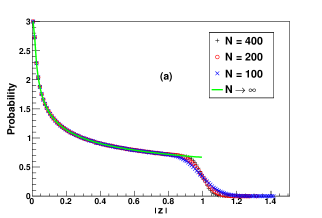
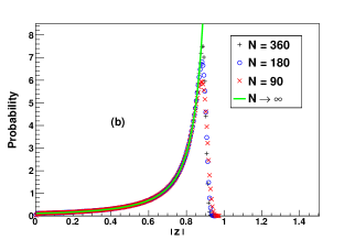
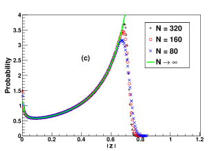
Figure 1: (Color online) Numerical verification of theoretical formulas (3) (a) and (4) (b),(c) for the radial part $p(r)=F^{\prime}(r)$ (7) of the mean spectral density $\rho\left(z,\bar{z}\right)$ of the product of independent matrices. (a) Numerical histograms for the product of 3 independent Gaussian random matrices $N=400$ (black crosses), $N=200$ (red circles) and $N=100$ (blue rotated crosses) compared to theoretical prediction for $N\rightarrow\infty$ (solid green line). Each histogram is made for $10^{7}$ eigenvalues. The numerical histograms approach theoretical curve as the size of matrices increases. (b) An analogous plot to (a) for the product of 2 independent truncated unitary matrices with ratio $\kappa=\frac{1}{9}$ and $N=360$ (black crosses), $N=180$ (red circles) and $N=90$ (blue rotated crosses). Each histogram is made for $9\times 10^{6}$ eigenvalues. (c) An analogous plot to (a) and (b) for the product of 3 independent truncated unitary matrices with ratio $\kappa=\frac{1}{4}$ and $N=320$ (black crosses), $N=160$ (red circles) and $N=80$ (blue rotated crosses). Each histogram represents $8\times 10^{6}$ eigenvalues.

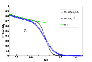
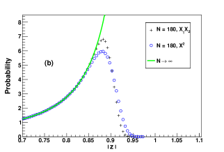
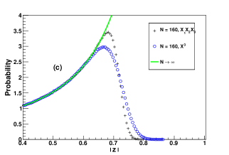
Figure 2: (Color online) Numerical analysis of the finite size effects for the radial part $p(r)=F^{\prime}(r)$ (7) of the mean spectral density $\rho\left(z,\bar{z}\right)$ of the product of independent matrices in comparison to the power of a single matrix. (a) Numerical histograms for product of 3 independent Gaussian random matrices $N=200$ (black crosses) and one matrix raised to 3’rd power for $N=200$ (blue circles) compared to theoretical prediction for $N\rightarrow\infty$ (solid green line). Each histogram is made for $10^{7}$ eigenvalues. Plots are zoomed in the region, where the difference in the shape is visible. (b) An analogous plot to (a) for the product of 2 independent truncated unitary matrices (black crosses) and 2’nd power of a single truncated unitary matrix (blue circles) with ratio $\kappa=\frac{1}{9}$ and $N=180$. Each histogram is made for $9\times 10^{6}$ eigenvalues. (c) An analogous plot to (a) and (b) but the product of 3 independent truncated unitary matrices (black crosses) and 3’rd power of a single truncated unitary matrix (blue circles) with ratio $\kappa=\frac{1}{4}$ and $N=160$. Each histogram is made for $8\times 10^{6}$ eigenvalues.

We also performed numerical simulations for the products of truncated orthogonal matrices as an example of multiplication of IOE matrices. In the large $N$ limit both the IUE and IOE densities are expected to have the same limiting distribution while for finite $N$ the distribution in the IOE case is expected to display a characteristic pattern that weakly breaks the circular symmetry of the eigenvalue distribution on the complex plane. More precisely, one expects that a fraction of eigenvalues accumulates on the real axis and disappears from a narrow depletion region close to the axis. The effect was first discussed for real Girko-Ginibre matrices e and later also for orthogonal truncated matrices ksz . It is known to be a finite size effect in the sense that the fraction of eigenvalues forming the pattern tends to zero for $N\rightarrow\infty$ so the full circular symmetry of the eigenvalue density is restored in the limit. In fact, this is exactly what we see in our numerical simulations of the product of truncated matrices. First we observe that the radial distribution of eigenvalues of product of two truncated unitary matrices is identical to the case of truncated orthogonal matrices except in a small region close to $r=0$ (see fig. 3.a). In figure 3.b we compare finite size distributions for the product of IUE (lower part) and IOE (upper part). We see that the IUE distribution is circularly symmetric up to the statistical noise while the IOE distribution has an elongated shape close to the real axis, as expected. Finally in fig. 3.c we show the full spectrum on which one can clearly see an accumulation of eigenvalues on the real axis.

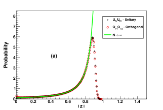
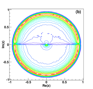
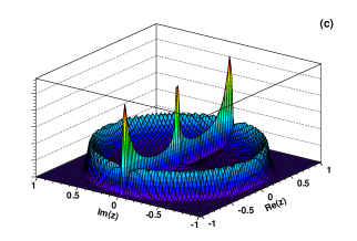
Figure 3: (Color online) Numerical comparison of the eigenvalues of product of two truncated orthogonal and unitary matrices. (a) The radial part $p(r)=F^{\prime}(r)$ (7) of the mean spectral density $\rho\left(z,\bar{z}\right)$ for unitary (black crosses) and orthogonal (red circles) matrices for $N=100$, $\kappa=\frac{1}{9}$. Each histogram is made for $9\times 10^{6}$ eigenvalues. The theoretical prediction for $N\rightarrow\infty$ is shown for comparison (solid green line). (b) Full eigenvalue distribution of orthogonal (upper half of complex plane) and unitary (lower half of complex plane) truncated matrices for $N=100$, $\kappa=\frac{1}{9}$. (c) Full eigenvalue distribution of orthogonal truncated matrices for same $N$,$\kappa$ parameters. The real eigenvalue band is clearly visible.

Discussion

In this note we have shown a simple, (and as far as we know) new relation between the spectral properties of the product of $n$ identically distributed isotropic random matrices from the given IUE ensemble and spectral properties of $n$-th power of a single matrix from this ensemble. We stress a nonintuitive aspect of this result that tells us that independent matrices, when multiplied, give the same eigenvalue density as the product of fully correlated (identical) matrices. In a sense it is a self-averaging effect: a single random matrix from a isotropic ensemble is a good representative to describe products of matrices from this ensemble in the limit $N\rightarrow\infty$. -

We have supplemented our analytic proof with extensive numerical simulations, allowing us to see how the finite size effects vanish in the thermodynamical limit. For Girko-Ginibre finite size effects agree with those conjectured in b1 ; b2 .

Our result elucidates the transparent analytic structure noted in several recently published papers on the products of random matrices bjw ; agt1 ; agt2 ; b1 ; b2 ; bjn ; os ; sz ; bmj ; bbcc ; ms ; gv ; fk ; djl and provides a powerful tool for the derivation of similar results for products of some application-designed, isotropic random matrices of large (infinite) size.

Acknowledgments

We thank Yan Fyodorov and Karol Zyczkowski for stimulating discussions. This work was supported by the Polish Ministry of Science Grant No. N N202 229137 (2009-2012) and by the Grant DEC-2011/02/A/ST1/00119 of National Centre of Science.

Appendix A

In this appendix we briefly recall basic facts about the S-transform, introduced by Voiculescu in free random probability v . Consider a Hermitian random matrix $a$. One usually defines the Green function

$$G_{a}(z)=\lim_{N\rightarrow\infty}\frac{1}{N}\left\langle\mbox{Tr}(z-a)^{-1}\right\rangle=\int d\lambda\frac{\rho_{a}(\lambda)}{z-\lambda}\ .$$ (27)

that is directly related to the eigenvalue density $\rho_{a}(\lambda)$. Note that the density is a function of a real variable while the Green’s function is a function of a complex variable. The Green’s function generates moments $\mu_{ak}$ (if they exist)

$$G_{a}(z)=\frac{1}{z}+\sum_{k=1}^{\infty}\frac{\mu_{ak}}{z^{k+1}}$$ (28)

of the eigenvalue density

$$\mu_{ak}=\lim_{N\rightarrow\infty}\frac{1}{N}\left\langle\mbox{Tr}\;a^{k}\right\rangle=\int d\lambda\rho_{a}(\lambda)\lambda^{k}\ .$$ (29)

Sometimes it is more convenient to use another generating function, given by a power series in $z$ rather than in $1/z$:

$$\psi_{a}(z)=\frac{1}{z}G_{a}\left(\frac{1}{z}\right)-1=\sum_{k=1}^{\infty}\mu_{ak}z^{k}$$ (30)

and to introduce its functional inverse $\chi_{a}$:

$$\chi_{a}(\phi_{a}(z))=\phi_{a}(\chi_{a}(z))=z$$ (31)

which can also be expressed as a power series in $z$ if the first moment is nonzero: $\mu_{a1}\neq 0$. The S-transform for the matrix $a$ is related to the $\chi$-transform as

$$S_{a}(z)=\frac{1+z}{z}\chi_{a}(z)\ .$$ (32)

The relevance of the S-transform in free probability is related to the fact that it allows one to concisely formulate the law of free multiplication. The S-transform of the product of two free (independent) matrices from invariant ensembles is a product of the S-transforms of individual matrices:

$$S_{ab}(z)=S_{a}(z)S_{b}(z)$$ (33)

The multiplication law was formulated in free random probability v but it also can be rederived in random matrix set-up using field theoretical techniques for the summation of planar Feynman diagrams and it can be generalized to non-hermitian matrices bjn .

Appendix B

In this appendix we rederive the distribution of a single unitary truncated matrix (23) using free probability and the Haagerup-Larsen theorem. We first construct the density of an $(N+L)\times(N+L)$ matrix $y=pu$ where

$$p=\mbox{diag}(\underbrace{1,\ldots,1}_{N},\underbrace{0,\ldots,0}_{L})$$ (34)

is a projection matrix and $u$ is an Haar unitary matrix of dimensions $(N+L)\times(N+L)$. In order to calculate the S-transform for the projector $p=p^{2}$ we first observe that all moments of $p$ are equal $\mu_{k}=N/(N+L)$. Hence $\psi_{p}(z)=\frac{N}{N+L}\frac{z}{1-z}$ (30), $\chi_{p}=\frac{z}{N/(N+L)+z}$ (31) and eventually (32)

$$S_{p}=\frac{1+z}{N/(N+L)+z}\ .$$ (35)

Inserting this to (5) we find

$$F_{y}(r)=\frac{L}{N+L}\frac{1}{1-r^{2}}\qquad\mbox{for}\quad r\leq\sqrt{N/(N+L)}$$ (36)

and $1$ otherwise. We see that $F_{y}(0)=L/(L+N)$. This means that there are $L$ eigenvalues equal zero. They are inherited from the zero eigenvalues of the projector. We can now reduce dimensionality of the matrix $y$ by removing $L$ zero eigenvectors. The remaining matrix $x$ that has no trivial zero eigenvalues. This gives the result given in equation (23) for a single truncated matrix

$$F_{x}(r)=\frac{N+L}{N}\left(F_{x}(r)-\frac{L}{N+L}\right)=\frac{L}{N}\frac{r^{2}}{1-r^{2}}\qquad\mbox{for}\quad r\leq\sqrt{N/(N+L)}$$ (37)

and one otherwise. The term $-L/(N+L)$ removes $L$ zero eigenvalues out of $(N+L)$ eigenvalues, and the factor $(N+L)/N$ restores the total normalization.

References

- (1) D. V. Voiculescu, K. J. Dykema and A. Nica, Free random variables, CRM Monograph Series, Vol. 1 (American Mathematical Society, Providence, RI, 1992). A non-commutative probability approach to free products with applications to random matrices, operator algebras and harmonic analysis on free groups.
- (2) F. Hiai and D. Petz, The semicircle law, free random variables and entropy, Mathematical Surveys and Monographs, Vol. 77, (American Mathematical Society, RI, 2000).
- (3) G. W. Anderson, A. Guionnet and O. Zeitouni, An Introduction to Random Matrices, (Cambridge University Press, UK, 2010).
- (4) A. Nica and R. Speicher, Lectures on the combinatorics of free probability, London Mathematical Society Lecture Note Series, Vol. 335 (Cambridge University Press, Cambridge, 2006).
- (5) U. Haagerup and F. Larsen, Journal of Functional Analysis, 176, 331 (2000).
- (6) Z. Burda, R. A. Janik, B. Waclaw, Phys. Rev. E 81, 041132 (2010).
- (7) N. Alexeev, F. Götze, A. Tikhomirov, Doklady Mathematics 82, 505 (2010).
- (8) N. Alexeev, F. Götze, A. Tikhomirov, Lithuanian Math. Journal, 50, 121 (2010).
- (9) J. Ginibre, J. Math. Phys. 6, (1965).
- (10) V. Girko, Theor. Prob. Appl. 29, 694 (1985).
- (11) J. Feinberg and A. Zee, Nucl.Phys. B 501, 643 (1997).
- (12) J. Feinberg, R. Scalettar, A. Zee, J.Math. Phys. 42, 5718 (2001).
- (13) A. Nica, R. Speicher, Fields Institute Communications, 12, 149 (1997).
- (14) A. Guionnet, M. Krishnapur and O. Zeitouni, Ann. Math. 174, 1189 (2011).
- (15) B. Collins, I. Nechita K. Zyczkowski, J. Phys. A 43, 275303 (2010).
- (16) K. A. Penson, K. Zyczkowski, Phys. Rev. E 83 061118 (2011).
- (17) K. Zyczkowski and H.-J. Sommers, J. Phys. A 33, 2045 (2000).
- (18) Z. Burda et al, Phys. Rev. E 82, 061114 (2010).
- (19) Z. Burda et al, Acta Phys. Polon. B 42, 939 (2011).
- (20) A. Edelman, J. Multivariate Anal. 60, 203 (1997).
- (21) B. A. Khoruzhenko, H.-J. Sommers and K. Zyczkowski, Phys. Rev. E 82, 040106 (2010).
- (22) Z. Burda, R. Janik and M.A. Nowak, Phys. Rev. E 84, 061125 (2011).
- (23) S. O’Rourke, A. Soshnikov, Electron. J. Probab. 16, 2219 (2011).
- (24) Z. D. Bai, B. Miao, B. Jin, J. Multivariate Anal. 98, 76 (2007).
- (25) T.Banica, S.Belinschi, M.Capitaine, B.Collins, Free Bessel laws, arXiv:0710.5931 (2007).
- (26) J.A. Mingo and R.Speicher, Sharp bounds for sums associated to graphs of matrices arXiv:0909.4277 (2009).
- (27) V. L. Girko, A.I. Vladimirova, Random Oper. Stochastic Equations 17, 243 (2009).
- (28) P. J. Forrester and M. Krishnapur, J. Phys. A: Math. Theor. 42, 385204 (2009).
- (29) Z. Dong, T. Jiang and D. Li, J. Math. Phys. 53, 013301 (2012).
- (30) D. V. Voiculescu, J. Operator Theory 18, 223 (1987).