Novel Disordering Mechanism in Ferromagnetic Systems with Competing Interactions

Abstract

Ferromagnetic Ising systems with competing interactions are considered in the presence of a random field. We find that in three space dimensions the ferromagnetic phase is disordered by a random field which is considerably smaller than the typical interaction strength between the spins. This is the result of a novel disordering mechanism triggered by an underlying spin-glass phase. Calculations for the specific case of the long-range dipolar ${{\rm LiHo_{x}Y_{1-x}F_{4}}}$ compound suggest that the above mechanism is responsible for the peculiar dependence of the critical temperature on the strength of the random field and the broadening of the susceptibility peaks as temperature is decreased, as found in recent experiments by Silevitch et al. [Nature (London) 448, 567 (2007)]. Our results thus emphasize the need to go beyond the standard Imry-Ma argument when studying general random-field systems.

Introduction.—

The random-field Ising model (RFIM) plays a central role in the study of disordered systems and has been applied to problems across disciplines ranging from disordered magnets to random pinning of polymers, as well as water seepage in porous media.

At and below the lower critical dimension $d_{\ell}=2$, the ferromagnetic (FM) phase is unstable to an infinitesimal random field (RF) Imry and Ma (1975); Binder (1983). At higher space dimensions the disordering of the FM phase requires the RF strength $h$ to be of the order of the spin-spin interaction strength $J$. Yet, the effect of the RF on the transition between the FM and paramagnetic (PM) phases—for systems with both short-range and dipolar interactions—has been source of vast experimental and theoretical scrutiny Nattermann (1988); Belanger (1998); Nattermann (1998). Over the past three decades the RFIM has been studied experimentally via dilute antiferromagnets in a field (DAFF) Fishman and Aharony (1979), as both the RFIM and the DAFF seem to share the same universality class. More recently it has been shown that in anisotropic dipolar magnets the RFIM can be realized in the FM phase: By applying a transverse field to a dilute dipolar ferromagnet, such as ${{\rm LiHo_{x}Y_{1-x}F_{4}}}$, one transforms the spatial disorder to a longitudinal effective RF Schechter and Laflorencie (2006); Tabei et al. (2006); Schechter (2008). This opens the doors for advancing our understanding of the RF problem com (a), as well as new applications, such as tunable domain-wall pinning Silevitch et al. (2010) in magnetic materials.

Silevitch et al. recently studied the FM-to-PM transition in the presence of RFs in ${{\rm LiHo_{x}Y_{1-x}F_{4}}}$ Silevitch et al. (2007). Remarkably, they found that $T_{c}$ depends linearly on the transverse field (and thus on $h$ Schechter and Laflorencie (2006); Schechter (2008)) and that the susceptibility peak diminishes and broadens as temperature decreases. In ${{\rm Mn_{12}\!-\!ac}}$, which is a realization of the RFIM with all FM interactions, a strong suppression of $T_{c}$ as a function of $h$ was found as well Wen et al. (2010), but with what appears to be a quite different functional dependence at small $h$.

Here we study the interplay between FM and spin-glass (SG) phases in a dipolar Ising model with competing interactions in the presence of a RF. We find a novel disordering mechanism of the FM phase when a RF is applied and the system is in close proximity (e.g., via dilution) to a SG phase. This disordering mechanism lies between the Imry-Ma and standard disordering mechanisms: The disordering of the FM phase occurs at a finite RF, which is considerably smaller than the typical spin-spin interaction, and the disordered phase [denoted henceforth as “quasi-SG” (QSG)] consists of not FM but glassy domains. At $T=0$ we predict the existence of a FM-to-QSG transition and determine for ${{\rm LiHo_{x}Y_{1-x}F_{4}}}$, analytically and numerically, the phase boundary as a function of the Ho concentration $x$ and RF strength $h$. At finite temperature our theory agrees with experiments Silevitch et al. (2007), suggesting that the existence of competing interactions and the proximity to the SG phase dictate the broadening of the susceptibility peaks at low temperature and the peculiar dependence of $T_{c}$ on $h$. Our theoretical analysis of the SG phase follows the scaling approach of Fisher and Huse Fisher and Huse (1988)—its validity supported by the agreement we find with our numerical results. The nature of the SG phase in a RF, however, is controversial Bhatt and Young (1985); Ciria et al. (1993); Kawashima and Young (1996); Billoire and Coluzzi (2003); Marinari et al. (1998); Houdayer and Martin (1999); Krzakala et al. (2001); Takayama and Hukushima (2004); Young and Katzgraber (2004); Katzgraber and Young (2005); Jörg et al. (2008); Katzgraber et al. (2009); Leuzzi et al. (2009, 2011); Baños et al. (2012); Larson et al. (2013), but of no concern here.

Theoretical analysis.—

We first study ${{\rm LiHo_{x}Y_{1-x}F_{4}}}$ at $T=0$. For dilutions $x>x_{c}$ the system is FM, whereas for $x_{0}<x<x_{c}$ the system is a SG. Below we show numerically that $x_{c}\approx 0.3$. To date, it is unclear if $x_{0}>0$ Stephen and Aharony (1981); Snider and Yu (2005). For $x\approx x_{c}$ we define the energy per spin of the lowest FM state of the system as $f_{\rm FM}(x)$, and the lowest energy of the SG state as $f_{\rm SG}(x)$. Note that $f_{\rm FM}(x)$ is the ground-state energy of the FM phase when $x>x_{c}$ and $f_{\rm SG}(x)$ represents the ground-state energy of the SG phase for $x_{0}<x<x_{c}$. At $x=x_{c}$ $f_{\rm FM}(x_{c})=f_{\rm SG}(x_{c})$, and for $x\approx x_{c}$, to first order in $x-x_{c}$, $f_{\rm SG}(x)-f_{\rm FM}(x)=\alpha(x-x_{c})+\ldots$. We consider the FM phase for $x>x_{c}$ in an applied RF of mean zero and standard deviation $h$. For small $h$, the FM state in three dimensions cannot gain energy from the field, because domain flips are not energetically favorable. However, for spin glasses the lower critical (Imry-Ma) dimension is infinity Fisher and Huse (1988). In particular, in 3D the energy of the system can be lowered by flipping domains, creating a QSG phase with a finite correlation length. Thus, for $x\sim x_{c}$ the energy of the SG state will become lower than the energy of the FM state at a finite RF, which is still considerably smaller than the typical spin-spin interaction $J$. More generally, any 3D Ising system with competing interactions having at zero RF a FM ground state and a SG state at a somewhat higher energy will be disordered through a transition to the QSG phase at a finite RF whose magnitude depends on the proximity to the SG phase and can be much smaller than $J$. Because in systems like ${{\rm LiHo_{x}Y_{1-x}F_{4}}}$ the effective RFs are a result of quantum fluctuations Schechter and Laflorencie (2006); Schechter et al. (2007), this phase transition is a particular case of a quantum phase transition where the quantum fluctuations of the spins are small, involving only the spin’s ground and first excited states com (b), but where the collective effect of all spins is strong enough to drive the transition.

The value of the critical RF can be estimated using the short-range Hamiltonian Binder and Young (1986) in a RF $H_{\rm EA}=-\sum_{\langle ij\rangle}J_{ij}S_{i}S_{j}+\sum_{i}h_{i}S_{i}$. $J_{ij}$ represent nearest-neighbor Gaussian random bonds between spins $S_{i}$ with zero mean and standard deviation $J$, and $h_{i}$ are Gaussian RFs of average strength $h$ com (c). The SG ground state is unstable to an infinitesimal RF, creating domains of typical size $(J/h)^{1/(3/2-\theta)}$ ($\theta\approx 0.19$) Hartmann (1999). The energy reduction per spin due to the RF is thus $f(h)=h(J/h)^{(-3/2)/(3/2-\theta)}$. The total energy reduction per spin is of the same order, because the energy cost to flip domains is much smaller. Considering now a FM system with competing interactions, e.g., ${{\rm LiHo_{x}Y_{1-x}F_{4}}}$ at $x>x_{c}$ where at $h=0$ the system is FM with $f_{\rm SG}>f_{\rm FM}$, the critical field $h_{c}(x)$ can be computed from $f(h=h_{c})=f_{\rm SG}-f_{\rm FM}$, i.e., $f(h=h_{c})=\alpha(x-x_{c})$. One obtains

$$h_{c}(x)=\alpha^{\prime}(J)(x-x_{c})^{(3/2-\theta)/(3-\theta)}\,,$$ (1)

where $\alpha^{\prime}(J)=\alpha^{(3/2-\theta)/(3-\theta)}J^{(3/2)/(3-\theta)}$; see Fig. 1. For $h>h_{c}(x)$ there are finite domains within which glassy order persists. The domain size decreases with increasing field, where at $h\approx J$ the system resembles a paramagnet. As $x\rightarrow x_{c}$, the disordering field approaches zero. For large $x-x_{c}$ and $h\approx J$ there is a crossover to the standard behavior where the disordering is a result of single-spin energy minimization; i.e., the intermediate QSG regime disappears.

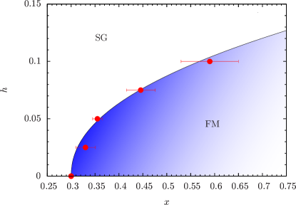
Figure 1: (color online) Comparison of the zero-temperature numerical and analytical [Eq. (1)] $h$-$x$ phase diagrams for the diluted dipolar Ising model [Eq. (2)]. $h_{c}(x)\sim(x-x_{c})^{0.466}$, with $\theta\approx 0.19$ Hartmann (1999). The analytical prediction agrees well with the numerical data ($\alpha^{\prime}$ is a fitting parameter).

We now consider finite temperatures and analyze the dependence of the FM $T_{c}$ (at $x>x_{c}$) on the effective RF. Let us denote the lowest free energies per spin of the FM phase (ordered for $T<T_{\rm FM}$, disordered for $T>T_{\rm FM}$) and a competing disordered QSG phase as $F_{\rm FM}(x,T)$ and $F_{\rm QSG}(x,T)$, respectively. Because the entropy of the QSG phase is dominated by regions at the boundaries between domains Fisher and Huse (1988), the main effect of the RFs is to lower the QSG energy. Thus, $F_{\rm QSG}(x,T)-F_{\rm FM}(x,T)=-A(T-T_{\rm FM})+B(x-x_{c})-h/\xi_{\rm QSG}^{3/2}$ [here, for $h=0$, $F_{\rm QSG}(x_{c},T_{c})=F_{\rm FM}(x_{c},T_{c})$]. For $h<h^{*}\equiv B(x-x_{c})\xi^{3/2}$ and $T=T_{\rm FM}$ we obtain $F_{\rm QSG}(x,T)>F_{\rm FM}(x,T)$, and the transition occurs between an ordered FM phase and a disordered PM phase dominated by FM fluctuations. However, for $h>h^{*}$ we obtain $T_{c}(h)-T_{c}(0)=A^{-1}\left[B(x-x_{c})-h/\xi^{3/2}\right]$, where the FM phase is disordered by a PM phase dominated by fluctuations of domains having SG correlations over distance $\xi$. Thus, at $h=h^{*}$, $T_{c}(h)$ has a crossover from a roughly quadratic dependence on the RF (known for a ferromagnet in a RF Ahrens et al. (2013)) to a linear dependence. This result is supported by our numerics.

Comparing to the experiments in Ref. Silevitch et al. (2007), our results are consistent with $T_{c}(h)$ being linear when $h\ll J$, with deviations from linearity as $h\rightarrow 0$. Note that in Ref. Silevitch et al. (2007) $T_{c}(h)$ is linear down to the lowest RFs studied if one defines $T_{c}$ by the asymptotic behavior of the susceptibility at high temperatures. However, if $T_{c}(h)$ is defined by the peak position of the susceptibility, deviations from linearity are observed at low fields com (d).

Numerical details.—

${{\rm LiHo_{x}Y_{1-x}F_{4}}}$ at low temperatures and in an external transverse magnetic field is well described by Chakraborty et al. (2004); Schechter (2008)

$$\!\!{\mathcal{H}}\!=\!\sum_{i\neq j}\frac{J_{ij}}{2}\epsilon_{i}\epsilon_{j}S_{i}S_{j}+\frac{J_{\rm ex}}{2}\!\!\sum_{\langle i,j\rangle}\epsilon_{i}\epsilon_{j}S_{i}S_{j}+\sum_{i}h_{i}\epsilon_{i}S_{i}\;.$$ (2)

Here $\epsilon_{i}=\left\{0,1\right\}$ is the occupation of the magnetic ${\rm Ho^{3+}}$ ions on a tetragonal lattice (lattice constants $a=b=5.175$Å and $c=10.75$Å) with four ions per unit cell Biltmo and Helenius (2009); Tam and Gingras (2009), $S_{i}\in\{\pm 1\}$, $h_{i}$ represent Gaussian RFs with zero mean and standard deviation $h$, where $h$ is measured in $[K]$. The magnetostatic dipolar coupling $J_{ij}$ between two ${\rm Ho^{3+}}$ ions is given by: $J_{ij}=D(r^{2}_{ij}-3z^{2}_{ij})/r_{ij}^{5}$, where $r_{ij}=|{\bf r}_{i}-{\bf r}_{j}|$, ${\bf r}_{i}$ is the position of the $i$th ${\rm Ho^{3+}}$ ion and $z_{ij}=\left({\bf r}_{i}-{\bf r}_{j}\right)\cdot\hat{z}$ is the component parallel to the easy axis. $D/a^{3}=0.214$K Biltmo and Henelius (2007) and the nearest-neighbor exchange is $J_{\rm ex}=0.12$K Biltmo and Helenius (2009); com (e). We use periodic boundary conditions with Ewald sums Tam and Gingras (2009); Wang and Holm (2001). At zero field and no dilution, we find $T_{c}=1.5316(2)$K, in agreement with experimental results where $T_{c}=1.530(5)$K Mennenga et al. (1984).

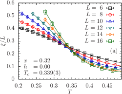
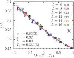
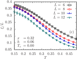
Figure 2: (color online) Correlation length $\xi_{L}/L$ as a function of $T$ for $x=0.32$. (a) $h=0$. There is a clear crossing for $T_{c}=0.340(3)$ com (e) for different system sizes $L$. (b) Scaling of the data for $h=0$. The solid line represents the optimal scaling function (polynomial approximation). (c) $h=0.06$. There is no transition.

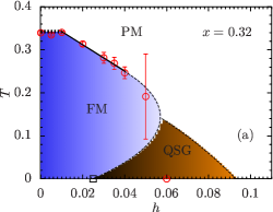
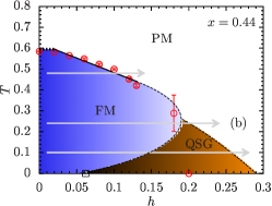
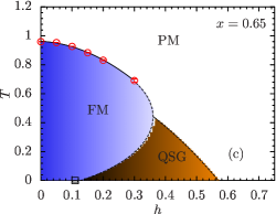
Figure 3: (color online) $T$-$h$ phase diagram of ${{\rm LiHo_{x}Y_{1-x}F_{4}}}$ for different concentrations $x$. Circles represent data from finite-temperature simulations, squares data from zero-temperature simulations (see Fig. 1). (a) $x=0.32$. (b) $x=0.44$ (dilution used in the experiments of Ref. Silevitch et al. (2007)). Horizontal lines denote lines of constant temperature and varying $h$, as done experimentally Silevitch et al. (2007) in susceptibility measurements. The top line has a direct FM-PM transition. The bottom two lines represent paths crossing the QSG phase where a broadening of the susceptibility peak and its diminishing with the enhancement of the RF at the crossover to the PM phase as temperature is decreased occur. (c) $x=0.65$. In all panels, dotted line segments represent the conjectured phase boundary.

For the zero-temperature simulations (Fig. 1) we use jaded extremal optimization Boettcher and Percus (2001); Middleton (2004). Here, $\tau=1.6$, $1.8$ and $2$ with an aging parameter $\Gamma=0.05$ for at least $2^{26}$ steps. Ground states are found with high confidence for $L\leq 10$ and $h=0$, and $L\leq 8$ with small $h\neq 0$. The phase boundary is identified via the Binder ratio $g=(1/2)(3-\left[{m^{4}}\right]_{\scriptscriptstyle\rm av}/\left[{m^{2}}\right]_{\scriptscriptstyle\rm av}^{2})$, where $m=(1/N)\sum_{i}S_{i}$ ($N=4xL^{3}$ is the number of spins and $\left[{\cdots}\right]_{\scriptscriptstyle\rm av}$ represents a disorder average. $g\sim\tilde{G}[L^{1/\nu}\left(x-x_{c}\right)]$ is a dimensionless function, allowing for the extraction of $x_{c}$ and $\nu$ for a fixed $h$. Parameters are listed in the Supplementary Material, Table 1 com (f).

At finite temperatures we use parallel tempering Monte Carlo Hukushima and Nemoto (1996). Parameters are listed in Tables 2, 3 and 4 in the Supplementary Material com (f). To determine the transitions for a given $h$ and $x$ we measure Ballesteros et al. (2000)

$$\xi_{L}=\frac{1}{2\sin(k_{\rm min}/2)}\sqrt{\frac{\left[{\left\langle{m^{2}(\mathbf{0})}\right\rangle_{\scriptscriptstyle\rm T}}\right]_{\scriptscriptstyle\rm av}}{\left[{\left\langle{m^{2}(\mathbf{k}_{\rm min})}\right\rangle_{\scriptscriptstyle\rm T}}\right]_{\scriptscriptstyle\rm av}}-1}\,,$$ (3)

where $m(\mathbf{k})=(1/N)\sum_{i=1}S_{i}\exp(i\mathbf{k}\cdot\mathbf{R}_{i})$. Here $\left\langle{\cdots}\right\rangle_{\scriptscriptstyle\rm T}$ represents a thermal average, and $\mathbf{R}_{i}$ is the spatial location of the spin $S_{i}$, and $\mathbf{k}_{\rm min}=(2\pi/L,0,0)$. $\xi_{L}/L\sim\tilde{X}[L^{1/\nu}(T-T_{c})]$; i.e., at the transition ($T=T_{c}$) the argument of $\tilde{X}$ is zero (up to scaling corrections) and hence independent of $L$ [lines of different system sizes cross [Fig. 2(a)]]. If, however, the lines do not meet, no transition occurs [Fig. 2(c)]. To determine $T_{c}(h)$ we scale the data [Fig. 2(b)]. Using a bootstrapped Levenberg-Marquardt minimization Katzgraber et al. (2006) allows us to determine the critical parameters with statistical errors; see Table 5 of the Supplemental Material com (f). Note that for a given $x$ the critical exponent $\nu$ increases with $h$.

Figure 1 shows the $h$-$x$ phase diagram of ${{\rm LiHo_{x}Y_{1-x}F_{4}}}$ at zero temperature. We find excellent agreement with Eq. (1), using $\theta\approx 0.19$ Hartmann (1999), i.e., $h_{c}(x)\sim(x-x_{c})^{0.466}$, and $\alpha^{\prime}$ a fitting parameter (quality of fit $Q=0.89$) Press et al. (1995). Note, however, that good fits are also possible for $0.42\lesssim z\lesssim 0.5$ with an optimal value of $z=0.43(4)$ ($Q=0.82$).

Figure 3 shows finite-temperature data for different $x$. Figure 3(a) shows $T_{c}(h)$ for $x=0.32$, i.e., $x-x_{c}=0.02$ small. Our results at finite $T$ corroborate our theoretical model with $h^{*}\approx 0.01$, where for $h<h^{*}$, $T_{c}$ is roughly independent of $h$ (at such small fields the numerical resolution does not allow a distinction between a constant and a parabolic dependence) and for $h>h^{*}$, $T_{c}(h)$ decreases linearly. The FM phase fully disorders, at all temperatures, for $h\approx 0.055(5)$, a value slightly larger than found from the $T=0$ simulations, yet much smaller than the interaction energy. Both the disordering of the FM phase at small fields and the linearity of $T_{c}(h)$ seem to persist up to $x=0.44$ [Fig. 3(b)], the dilution used in Ref. Silevitch et al. (2007), albeit with a less pronounced crossover at $h=h^{*}$. For $x=0.65$ [far from the SG phase, Fig. 3(c)] the behavior of $T_{c}(h)$ changes to a quadratic dependence for all $h<0.3$, suggesting a standard FM-PM transition. Critical parameters are listed in the Supplemental Material, Table 5 com (f).

Phase diagram: Reentrance and experiment.—

Our analysis for zero RF suggests that the critical concentration $x_{c}=0.3$ separating the FM and SG phases depends only slightly, if at all, on temperature. Reentrance to a SG phase is either missing or limited to a small concentration regime, in contrast to previous suggestions Reich et al. (1990).

At the same time, our results at finite RF at both zero and finite temperature for all concentrations suggest that there is a range of RFs where the system shows reentrance to a frozen QSG phase at low temperatures com (g). The RF-temperature phase diagram is shown in Fig. 3. Note also that the PM phase is characterized by distinct correlations over the phase diagram: FM fluctuating domains close to the FM phase at $h<h^{*}$ [dashed line in Figs. 3(a) and 3(b)], and SG fluctuating domains close to the transition for $h>h^{*}$. This form of the phase diagram is strongly supported by, and provides an explanation for, the results of Ref. Silevitch et al. (2007), Fig. 2. For $T>0.3$K [inflection point in Fig. 3(b) above] there is a direct transition from the FM to the PM [top horizontal arrow in Fig. 3(b)], as is indeed marked experimentally by a sharp cusp in the magnetic susceptibility. For $T<0.3$K, however, as the transverse field (and correspondingly the effective RF) is increased, the FM phase changes into a frozen QSG phase and only then to the PM phase [central horizontal arrow in Fig. 3(b)]. Experimentally, this effect is mirrored by a broad peak in the susceptibility at $T<0.3$K, in good agreement with the inflection point we find at $x=0.44$. As temperature is further reduced, the crossover between the frozen QSG phase and the PM phase occurs at a larger RF [bottom horizontal arrow in Fig. 3(b)], resulting in smaller glassy domains and the experimentally observed diminishing peak of the susceptibility Wu et al. (1993); Schechter and Laflorencie (2006).

Conclusions.—

We propose a novel disordering mechanism for 3D ferromagnets with competing interactions and an underlying spin-glass phase, resulting in a disordering field which is finite, yet can be much smaller than the interaction strength. We explain various aspects of the experiments of Ref. Silevitch et al. (2007), including the peculiar linear dependence of $T_{c}$ on the applied transverse field and the diminishing and broadening of the susceptibility peak with decreasing temperature. We further find that at smaller concentrations ($x=0.32$, close to the spin-glass phase) the reduction of $T_{c}$ with the RF becomes more pronounced. Our results strongly support the notion that it is the interplay between the competing interactions and the induced effective RF that dictate the behavior of the ${{\rm LiHo_{x}Y_{1-x}F_{4}}}$ ferromagnet at low concentrations. Our analytical results are generic to FM systems with competing interactions. It would therefore be interesting to verify these results for other types of interactions and lattice structurescom (h).

 

Supplementary Material: Andresen et al.

Table 1: Simulation parameters for $T=0$: System of size $L=6$, $8$, and $10$, field $h$ and dilution $x$ are studied. $x_{\rm min}$ [$x_{\rm max}$] is the smallest [largest] concentration studied and $\Delta x$ is the step size between measurements. $N_{\rm sa}$ is the number of disorder realizations.

$h$	$x_{\rm min}$	$x_{\rm max}$	$\Delta x$	$N_{\rm sa}$
$0.000$	$0.280$	$0.350$	$0.010$	$5000$
$0.025$	$0.275$	$0.400$	$0.025$	$3000$
$0.050$	$0.300$	$0.400$	$0.025$	$3000$
$0.075$	$0.300$	$0.600$	$0.050$	$1500$
$0.100$	$0.400$	$0.800$	$0.100$	$1500$

Table 2: Simulation parameters at finite temperature and $x=0.32$ for different fields $h$ and system sizes $L$. The equilibration/measurement times are $2^{b}$ Monte Carlo sweeps. $T_{\rm min}$ [$T_{\rm max}$] is the lowest [highest] temperature used and $N_{T}$ is the number of temperatures. $N_{\rm sa}$ is the number of disorder realizations.

$x$	$h$	$L$	$b$	$T_{\rm min}$	$T_{\rm max}$	$N_{T}$	$N_{\rm sa}$
$0.32$	$0.000$	$6$	$15$	$0.100$	$0.500$	$25$	$2000$
$0.32$	$0.000$	$8$	$17$	$0.100$	$0.500$	$25$	$2000$
$0.32$	$0.000$	$10$	$18$	$0.168$	$0.500$	$20$	$1000$
$0.32$	$0.000$	$12$	$18$	$0.240$	$0.500$	$15$	$1000$
$0.32$	$0.000$	$14$	$16$	$0.275$	$0.500$	$10$	$750$
$0.32$	$0.000$	$16$	$16$	$0.275$	$0.500$	$10$	$385$
$0.32$	$0.005$	$6$	$12$	$0.280$	$0.550$	$20$	$2000$
$0.32$	$0.005$	$8$	$13$	$0.280$	$0.550$	$20$	$3500$
$0.32$	$0.005$	$10$	$15$	$0.280$	$0.550$	$20$	$2000$
$0.32$	$0.005$	$12$	$17$	$0.280$	$0.550$	$20$	$1200$
$0.32$	$0.005$	$14$	$16$	$0.312$	$0.550$	$17$	$1200$
$0.32$	$0.010$	$6$	$15$	$0.050$	$0.500$	$30$	$1500$
$0.32$	$0.010$	$8$	$17$	$0.050$	$0.500$	$30$	$1100$
$0.32$	$0.010$	$10$	$18$	$0.230$	$0.500$	$15$	$1000$
$0.32$	$0.010$	$12$	$19$	$0.245$	$0.500$	$15$	$850$
$0.32$	$0.010$	$14$	$17$	$0.265$	$0.500$	$15$	$750$
$0.32$	$0.020$	$6$	$15$	$0.050$	$0.500$	$30$	$1500$
$0.32$	$0.020$	$8$	$18$	$0.050$	$0.500$	$30$	$1000$
$0.32$	$0.020$	$10$	$16$	$0.245$	$0.500$	$15$	$1000$
$0.32$	$0.020$	$12$	$19$	$0.245$	$0.500$	$15$	$600$
$0.32$	$0.020$	$14$	$17$	$0.274$	$0.500$	$13$	$7500$
$0.32$	$0.030$	$6$	$14$	$0.226$	$0.450$	$14$	$3000$
$0.32$	$0.030$	$8$	$17$	$0.212$	$0.450$	$15$	$2000$
$0.32$	$0.030$	$10$	$17$	$0.226$	$0.450$	$14$	$2000$
$0.32$	$0.030$	$12$	$19$	$0.226$	$0.450$	$14$	$600$
$0.32$	$0.035$	$6$	$13$	$0.218$	$0.450$	$20$	$3000$
$0.32$	$0.035$	$8$	$14$	$0.218$	$0.450$	$20$	$2000$
$0.32$	$0.035$	$10$	$15$	$0.218$	$0.450$	$20$	$2000$
$0.32$	$0.035$	$12$	$18$	$0.218$	$0.450$	$20$	$650$
$0.32$	$0.040$	$6$	$14$	$0.218$	$0.450$	$20$	$3000$
$0.32$	$0.040$	$8$	$16$	$0.218$	$0.450$	$20$	$2800$
$0.32$	$0.040$	$10$	$17$	$0.218$	$0.450$	$20$	$2000$
$0.32$	$0.040$	$12$	$17$	$0.218$	$0.450$	$14$	$1000$
$0.32$	$0.050$	$6$	$13$	$0.105$	$0.500$	$20$	$1500$
$0.32$	$0.050$	$8$	$16$	$0.150$	$0.500$	$20$	$1000$
$0.32$	$0.050$	$10$	$18$	$0.150$	$0.500$	$20$	$1000$
$0.32$	$0.050$	$12$	$19$	$0.150$	$0.500$	$20$	$1000$
$0.32$	$0.060$	$6$	$12$	$0.150$	$0.500$	$20$	$2000$
$0.32$	$0.060$	$8$	$16$	$0.150$	$0.500$	$20$	$2000$
$0.32$	$0.060$	$10$	$19$	$0.150$	$0.500$	$20$	$2000$
$0.32$	$0.060$	$12$	$20$	$0.150$	$0.500$	$20$	$1000$

Table 3: Simulation parameters at finite temperature and $x=0.44$. For details see Table 2.

$x$	$h$	$L$	$b$	$T_{\rm min}$	$T_{\rm max}$	$N_{T}$	$N_{\rm sa}$
$0.44$	$0.000$	$6$	$10$	$0.500$	$1.000$	$30$	$1000$
$0.44$	$0.000$	$8$	$12$	$0.500$	$1.000$	$30$	$1300$
$0.44$	$0.000$	$10$	$13$	$0.500$	$1.000$	$30$	$2500$
$0.44$	$0.000$	$12$	$14$	$0.500$	$1.000$	$30$	$550$
$0.44$	$0.000$	$14$	$14$	$0.560$	$1.000$	$47$	$650$
$0.44$	$0.020$	$6$	$10$	$0.525$	$0.800$	$30$	$2000$
$0.44$	$0.020$	$8$	$12$	$0.525$	$0.800$	$30$	$2000$
$0.44$	$0.020$	$10$	$13$	$0.525$	$0.800$	$30$	$1000$
$0.44$	$0.020$	$12$	$14$	$0.525$	$0.800$	$30$	$1000$
$0.44$	$0.020$	$14$	$14$	$0.550$	$0.800$	$30$	$900$
$0.44$	$0.040$	$6$	$11$	$0.525$	$0.750$	$22$	$2000$
$0.44$	$0.040$	$8$	$12$	$0.525$	$0.750$	$22$	$2000$
$0.44$	$0.040$	$10$	$14$	$0.540$	$0.750$	$20$	$1000$
$0.44$	$0.040$	$12$	$15$	$0.550$	$0.750$	$20$	$1000$
$0.44$	$0.060$	$6$	$11$	$0.500$	$0.750$	$25$	$2000$
$0.44$	$0.060$	$8$	$13$	$0.500$	$0.750$	$25$	$2000$
$0.44$	$0.060$	$10$	$13$	$0.519$	$0.730$	$19$	$2000$
$0.44$	$0.060$	$12$	$14$	$0.519$	$0.730$	$19$	$1300$
$0.44$	$0.080$	$6$	$12$	$0.475$	$0.725$	$20$	$2000$
$0.44$	$0.080$	$8$	$13$	$0.475$	$0.725$	$20$	$2000$
$0.44$	$0.080$	$10$	$13$	$0.500$	$0.725$	$20$	$1200$
$0.44$	$0.080$	$12$	$14$	$0.509$	$0.725$	$19$	$1300$
$0.44$	$0.100$	$6$	$13$	$0.445$	$0.725$	$23$	$2000$
$0.44$	$0.100$	$8$	$14$	$0.445$	$0.725$	$23$	$2300$
$0.44$	$0.100$	$10$	$13$	$0.445$	$0.725$	$23$	$2200$
$0.44$	$0.100$	$12$	$15$	$0.475$	$0.725$	$20$	$880$
$0.44$	$0.120$	$6$	$13$	$0.425$	$0.725$	$30$	$2500$
$0.44$	$0.120$	$8$	$14$	$0.425$	$0.725$	$30$	$2200$
$0.44$	$0.120$	$10$	$15$	$0.425$	$0.725$	$30$	$1000$
$0.44$	$0.120$	$12$	$16$	$0.445$	$0.725$	$25$	$1000$
$0.44$	$0.130$	$6$	$13$	$0.375$	$0.750$	$20$	$2000$
$0.44$	$0.130$	$8$	$15$	$0.375$	$0.750$	$20$	$1000$
$0.44$	$0.130$	$10$	$16$	$0.375$	$0.750$	$20$	$1000$
$0.44$	$0.180$	$6$	$14$	$0.270$	$0.750$	$45$	$3000$
$0.44$	$0.180$	$8$	$16$	$0.270$	$0.750$	$45$	$1500$
$0.44$	$0.180$	$10$	$19$	$0.270$	$0.750$	$45$	$512$
$0.44$	$0.200$	$6$	$14$	$0.270$	$0.750$	$45$	$3000$
$0.44$	$0.200$	$8$	$16$	$0.270$	$0.750$	$45$	$2000$
$0.44$	$0.200$	$10$	$19$	$0.270$	$0.750$	$45$	$512$

Table 4: Simulation parameters at finite temperature and $x=0.65$. For details see Table 2.

$x$	$h$	$L$	$b$	$T_{\rm min}$	$T_{\rm max}$	$N_{T}$	$N_{\rm sa}$
$0.65$	$0.000$	$6$	$10$	$0.500$	$1.400$	$20$	$1000$
$0.65$	$0.000$	$8$	$12$	$0.500$	$1.400$	$20$	$500$
$0.65$	$0.000$	$10$	$12$	$0.500$	$1.400$	$20$	$450$
$0.65$	$0.000$	$12$	$11$	$0.500$	$1.400$	$20$	$500$
$0.65$	$0.000$	$14$	$10$	$0.850$	$1.400$	$15$	$490$
$0.65$	$0.000$	$16$	$11$	$0.850$	$1.400$	$15$	$470$
$0.65$	$0.050$	$6$	$8$	$0.697$	$1.400$	$15$	$1000$
$0.65$	$0.050$	$8$	$10$	$0.697$	$1.400$	$15$	$500$
$0.65$	$0.050$	$10$	$9$	$0.800$	$1.400$	$20$	$500$
$0.65$	$0.050$	$12$	$11$	$0.697$	$1.400$	$15$	$300$
$0.65$	$0.050$	$14$	$10$	$0.900$	$1.400$	$15$	$500$
$0.65$	$0.050$	$16$	$11$	$0.920$	$1.400$	$16$	$280$
$0.65$	$0.100$	$6$	$8$	$0.820$	$1.400$	$20$	$750$
$0.65$	$0.100$	$8$	$9$	$0.820$	$1.400$	$20$	$500$
$0.65$	$0.100$	$10$	$10$	$0.820$	$1.400$	$20$	$500$
$0.65$	$0.100$	$12$	$11$	$0.820$	$1.400$	$20$	$800$
$0.65$	$0.100$	$14$	$12$	$0.820$	$1.400$	$20$	$380$
$0.65$	$0.150$	$6$	$8$	$0.820$	$1.400$	$20$	$1000$
$0.65$	$0.150$	$8$	$10$	$0.820$	$1.400$	$20$	$500$
$0.65$	$0.150$	$10$	$11$	$0.820$	$1.400$	$20$	$500$
$0.65$	$0.150$	$12$	$12$	$0.820$	$1.400$	$20$	$500$
$0.65$	$0.150$	$14$	$13$	$0.820$	$1.400$	$20$	$500$
$0.65$	$0.200$	$6$	$10$	$0.661$	$1.400$	$15$	$500$
$0.65$	$0.200$	$8$	$11$	$0.661$	$1.400$	$15$	$400$
$0.65$	$0.200$	$10$	$14$	$0.756$	$1.400$	$13$	$1300$
$0.65$	$0.200$	$12$	$15$	$0.756$	$1.400$	$13$	$1000$
$0.65$	$0.200$	$14$	$16$	$0.756$	$1.400$	$13$	$990$
$0.65$	$0.300$	$6$	$10$	$0.600$	$1.400$	$20$	$750$
$0.65$	$0.300$	$8$	$15$	$0.600$	$1.400$	$20$	$1000$
$0.65$	$0.300$	$10$	$17$	$0.600$	$1.400$	$20$	$550$
$0.65$	$0.300$	$12$	$19$	$0.600$	$1.400$	$20$	$530$

Table 5: Critical parameters estimated using a finite-size scaling technique: For each concentration $x$ and field strength $h$ we compute the critical temperature $T_{c}$ and critical exponent $\nu$.

$x$	$h$	$T_{c}$	$\nu$
$0.32$	$0.000$	$0.340(3)$	$0.83(3)$
$0.32$	$0.005$	$0.335(3)$	$0.89(3)$
$0.32$	$0.010$	$0.340(3)$	$0.81(3)$
$0.32$	$0.020$	$0.314(5)$	$1.04(7)$
$0.32$	$0.030$	$0.281(13)$	$1.23(17)$
$0.32$	$0.035$	$0.269(14)$	$1.31(19)$
$0.32$	$0.040$	$0.247(14)$	$1.41(15)$
$0.44$	$0.000$	$0.584(1)$	$0.75(1)$
$0.44$	$0.020$	$0.581(1)$	$0.70(1)$
$0.44$	$0.040$	$0.563(3)$	$0.77(2)$
$0.44$	$0.060$	$0.548(5)$	$0.86(3)$
$0.44$	$0.080$	$0.522(5)$	$0.99(4)$
$0.44$	$0.100$	$0.506(5)$	$1.01(4)$
$0.44$	$0.120$	$0.466(9)$	$1.39(12)$
$0.65$	$0.000$	$0.9597(8)$	$0.79(2)$
$0.65$	$0.050$	$0.9531(10)$	$0.76(2)$
$0.65$	$0.100$	$0.9264(14)$	$0.84(3)$
$0.65$	$0.150$	$0.8832(21)$	$0.91(4)$
$0.65$	$0.200$	$0.8312(41)$	$1.06(10)$
$0.65$	$0.300$	$0.6905(113)$	$1.11(12)$