Locating a single facility and a high-speed line

Abstract

In this paper we study a facility location problem in the plane in which a single point (facility) and a rapid transit line (highway) are simultaneously located in order to minimize the total travel time from the clients to the facility, using the $L_{1}$ or Manhattan metric. The rapid transit line is given by a segment with any length and orientation, and is an alternative transportation line that can be used by the clients to reduce their travel time to the facility. We study the variant of the problem in which clients can enter and exit the highway at any point. We provide an $O(n^{3})$-time algorithm that solves this variant, where $n$ is the number of clients. We also present a detailed characterization of the solutions, which depends on the speed given in the highway.

1 Introduction

Suppose we are given a set of clients represented as a set of points in the plane, and a service facility represented as a point to which all clients have to move. Every client can reach the facility directly, or use an alternative rapid transit line called highway in order to reduce the travel time. The highway is a straight line segment of arbitrary orientation. If a client moves directly to the facility, it moves at unit speed and the distance traveled is the Manhattan or $L_{1}$ distance to the facility. In the case where a client uses the highway, it travels the $L_{1}$ distance at unit speed to one point of the highway, traverses with a speed $v>1$ the Euclidean distance to other highway point, and finally travels the $L_{1}$ distance from that point to the facility at unit speed. All clients traverse the highway at the same speed. The highway is used by a client point whenever it saves time to reach the facility. Given the set of points representing the clients, the facility location problem consists in determining at the same time the facility point and the highway in order to minimize the total weighted travel time from the clients to the facility. The weighted travel time of a client is its travel time multiplied by a weight representing the intensity of its demand.

Recent papers have dealt with geometric problems considering travelling distances as a combination of planar and network distances. Carrizosa and Rodríguez-Chía [10] introduced the $p$-facility min-sum location problem on the plane with a metric induced by a gauge and a finite set of rapid transit lines giving the network distance. This problem was further developed by Gugat and Pfeiffer [15], and Pfeiffer and Klamroth [21]. Brimberg et al. [7, 8] studied the location of a new single facility considering given regions of distinct distance measures. All these papers consider the well-known Weber problem under a new metric. Other papers can be found in the context of the combination of the $L_{1}$ distance with the network distance. Abellanas et al. [1] introduced the time metric model: Given an underlying metric, the user can travel at speed $\nu(h)$ when moving along a highway $h$ or unit speed elsewhere. The particular case in which the underlying metric is the $L_{1}$ metric and all highways are axis-parallel segments of the same speed, is called the city metric [4]. In the scenario of setting up an optimal distance network that minimizes the maximum travel time among a set of points, several problems have been recently investigated in detail [3, 5, 9]. Other similar and more general models were studied by Korman and Tokuyama [18]. See [17] and [13] for surveys on highway location and extensive facility location problems, respectively.

A similar problem consisting in simultaneously locating a service facility point and a high-speed line (i.e. highway) of fixed length was recently studied by Espejo and Rodríguez-Chía [14] and Díaz-Báñez et al. [12]. The authors considered that highway is a turnpike [18], that is, clients can enter and exit the highway only at the endpoints. A first solution was introduced by Espejo and Rodríguez-Chía, and after that an improved solution was given by Díaz-Báñez et al. The problem aims to minimize the total weighted travel time from the demand points to the facility service, and can be solved in $O(n^{3})$ time [12], where $n$ is the number of clients. Díaz-Báñez et al. [11] continued the study of this variant by considering the min-max optimization criterion. They minimize the maximum time distance from the clients to the facility point.

In this paper we study a related problem in which the length of the highway is variable, that is, it is not fixed in advance as part of the input of the problem, and clients can enter and exit the highway at any point. Due to the latter condition, highway is called freeway [18]. Since both entering and leaving the highway are allowed at all its points, then the structure (i.e. highway) is continuously integrated in the plane. We minimize the total weighted transportation time from the demand points to the facility. The problem of locating a min-max freeway of fixed length was solved by Díaz-Báñez et al. [11] in $O(n\log n)$ time.

The following notation is introduced in order to formulate the problem. Let $S$ be the set of $n$ demand points, $f$ be the service facility point, $h$ be the highway, and $v>1$ be the speed in which demand points move along $h$. Given a demand point $p$, $w_{p}>0$ denotes the weight of $p$. The travel time between a demand point $p$ and the service facility $f$, denoted by $d_{h}(p,f)$, is equal to:

$$\min\left\{\begin{array}[]{l}\|p-f\|_{1},\\ \min_{q_{1},q_{2}\in h}\left\{\|p-q_{1}\|_{1}+\frac{\|q_{1}-q_{2}\|_{2}}{v}+\|q_{2}-f\|_{1}\right\}\end{array}\right.$$ (1)

The problem can be formulated as follows:

The Freeway and Facility Location problem (FFL-problem) Given a set $S$ of $n$ demand points, the weight $w_{p}>0$ of each point $p$ of $S$, and fixed speed $v>1$, locate the facility point $f$ and the highway $h$ in order to minimize the next function:

$$\Phi(f,h):=\sum_{p\in S}w_{p}\cdot d_{h}(p,f).$$ (2)

Our results.

We first show that there exist optimal solutions of the FFL-problem in which the highway $h$ has infinite length and the facility point $f$ is located on $h$. We then consider only optimal solutions satisfying these properties. We second show that for all demand points $p$ the shortest path from $p$ to the facility point $f$ has one of three possible shapes: (a) $p$ moves directly to $f$, (b) $p$ first moves vertically to reach $h$ and after that moves along $h$ to reach $f$, and (c) $p$ first moves horizontally to reach $h$ and after that moves along $h$ to reach $f$. For each demand point, the shape of its shortest time path to $f$ depends on both the speed $v$ in which demand points moves along $h$ and the slope of $h$. This discretization on the shortest path shapes allows us to simplify the expression of $d_{h}(p,f)$ and then to obtain a clear expression of the objective function $\Phi(f,h)$. Using geometric obervations, we reduce the search space of the optimal solutions. This is done by considering the grid $G$ defined by all axis-parallel lines passing through the demand points. We prove the existence of optimal solutions $(f,h)$ that satisfy one of the following two properties: (1) $h$ passes through a demand point and $f$ belongs to a line of grid $G$, and (2) $f$ is a vertex of $G$. The discretization of the search space permits us to obtain the main result of this paper, a general $O(n^{3})$-time algorithm to solve the FFL-problem. Our algorithm divides the search into two cases that correspond to the above two properties. As a surprising result, we prove that when speed $v$ is greater than $\frac{3\sqrt{2}}{4}\approx 1.060660172$ the algorithm can avoid the search of optimal solutions satisfying property (2) because in that case there always exists an optimal solution which holds property (1). This result simplifies the algorithm when speed exceeds that bound. We finally present three examples, two of them showing that when speed is increased and we keep the same configuration of demand points the shapes of the shortest time paths can change. A third example shows that when speed is less than $\frac{3\sqrt{2}}{4}$, there exist configurations in which the optimal solution satisfies property (2).

Outline.

The discretization on the shapes of the shortest paths from the demand points to the facility is stated in Section 2. In Section 3 we show how the search space of optimal solutions can be reduced. In Section 4 the algorithm to solve the FFL-problem is presented and in Section 5 we give the refinement of it. In Section 6, the examples are presented. Finally, in Section 7, we present the conclusions and further research.

2 Discretization of the shortest paths

Any solution to our problem will be encoded by a pair of elements $(f,h)$, where $f$ is the facility point and $h$ is the highway. Given $f$ and $h$, we say that a demand point $p$ does not use $h$ (or goes directly to $f$) if $d_{h}(p,f)$ is equal to $\|p-f\|_{1}$. Otherwise we say that $p$ uses $h$. Given any point $u$ of the plane, let $x_{u}$ and $y_{u}$ denote the $x-$ and $y-$coordinates of $u$, respectively.

Claim 2.1

Let $p_{1}$ and $p_{2}$ be demand points using the highway $h$ such that they move in contrary directions along $h$. Let segments $s_{1},s_{2}\subseteq h$ denote the portions of $h$ traversed by $p_{1}$ and $p_{2}$, respectively. Segments $s_{1}$ and $s_{2}$ have disjoint interiors.

Proposition 2.2

There exists an optimal solution of the FFL-problem in which the facility point is located on the highway.

• Let $(f,h)$ denote an optimal solution of the FFL-problem and suppose that $f$ does not belong to $h$. Let $h^{\prime}$ be a translation of $h$ such that $f$ belongs to $h^{\prime}$. We select $h^{\prime}$ so that to satisfy a condition that will be stated later. Let $p$ be a demand point. If $p$ does not use $h$ then:

  $$d_{h^{\prime}}(p,f)\leq\|p-f\|_{1}=d_{h}(p,f).$$ (3)

  Otherwise, if $p$ uses $h$, let $q_{1},q_{2}\in h$ be points such that

  $$d_{h}(p,f)=\|p-q_{1}\|_{1}+\frac{\|q_{1}-q_{2}\|_{2}}{v}+\|q_{2}-f\|_{1}.$$

  Let $q_{3}$ be the point $f+(q_{1}-q_{2})$, which belongs to the line containing $h^{\prime}$. Observe from Claim 2.1 that we can select $h^{\prime}$ so that point $q_{3}$ belongs to $h^{\prime}$ for every demand point $p$ using $h$. Then, by using the triangular inequality with the $L_{1}$ metric, we obtain:

  $$d_{h^{\prime}}(p,f) \leq \|p-q_{3}\|_{1}+\frac{\|q_{3}-f\|_{2}}{v}$$ (4)

  $$= \|p-q_{1}+(q_{2}-f)\|_{1}+\frac{\|q_{1}-q_{2}\|_{2}}{v}$$

  $$\leq \|p-q_{1}\|_{1}+\frac{\|q_{1}-q_{2}\|_{2}}{v}+\|q_{2}-f\|_{1}$$

  $$= d_{h}(p,f)$$

  From equations (7) and (4) we have $\Phi(f,h^{\prime})=\sum_{p\in S}w_{p}\cdot d_{h^{\prime}}(p,f)\leq\sum_{p\in S}w_{p}\cdot d_{h}(p,f)=\Phi(f,h)$. Then the pair $(f,h^{\prime})$ must be an optimal solution and the result thus follows.  ${\square}$

Results similar to Propostion 2.2, stating that the facility point belongs to the corresponding highway, can be found in [11, 14]. Observe from equations (2) and (7) that there always exists an optimal solution $(f,h)$ to the FFL-problem in which the length of $h$ is infinite. We then assume from this point forward that every solution satisfies that the highway is a straight line and the facility point belongs to the highway. Observe that this assumption does not have negative consequences, due to the fact that in practice a highway of infinite length is not possible. In fact, if a solution $(f,h)$ to the problem is such that $h$ is a straight line, then $(f,h^{\prime\prime})$ is also an optimal solution, where $h^{\prime\prime}\subset h$ is the segment of minimum length such that every demand point both enter and exit $h$ on a point of $h^{\prime\prime}$.

Let $\alpha$ always denote the non-negative angle of the highway with respect to the positive direction of the $x$-axis. Unless otherwise specified, we assume $0\leq\alpha\leq\frac{\pi}{4}$. Observe that if $\alpha>\frac{\pi}{4}$ we can, by properties of $L_{1}$ and $L_{2}$ metrics, modify the coordinate system so that angle $\alpha$ satisfies $0\leq\alpha\leq\frac{\pi}{4}$.

Given highway $h$ and a demand point $p$, let $p^{\prime}$ be the intersection point between $h$ and the vertical line passing through $p$. Similarly, let $p^{\prime\prime}$ be the intersection point between $h$ and the horizontal line passing through $p$. Let $h_{p^{\prime}}$ denote the half-line contained in $h$ that emanates from $p^{\prime}$ and does not contain $p^{\prime\prime}$, and $h_{p^{\prime\prime}}$ denote the half-line contained in $h$ that emanates from $p^{\prime\prime}$ and does not contain $p^{\prime}$. Notice from the assumption $0\leq\alpha\leq\frac{\pi}{4}$ that given $h$ and a demand point $p$, $p^{\prime}$ is the nearest point to $p$ on $h$ under the $L_{1}$ metric.

The next lemma characterizes the way in which demand points move optimally to the facility. Let $\varphi_{v}=\frac{\pi}{4}-\arcsin\left(\frac{\sqrt{2}}{2v}\right)$. Since $v>1$ we have $0<\varphi_{v}<\frac{\pi}{4}$.

Lemma 2.3

Given the highway $h$ and the facility point $f$ located on $h$, the following holds for all demand points $p$. If $0\leq\alpha\leq\varphi_{v}$ then $p$ moves first to $p^{\prime}$ and after that moves to $f$ using $h$. Otherwise, if $\varphi_{v}<\alpha\leq\frac{\pi}{4}$, the next statements are true:

• If $f\in h_{p^{\prime}}$ then $p$ moves first to $p^{\prime}$ and after that moves to $f$ using $h$.

• If $f\in h_{p^{\prime\prime}}$ then $p$ moves first to $p^{\prime\prime}$ and after that moves to $f$ using $h$.

• If $f\in h\setminus(h_{p^{\prime}}\cup h_{p^{\prime\prime}})$ then $p$ moves directly to $f$ without using $h$.

• Let $p$ be a demand point and assume w.l.o.g. that $p$ is below $h$. Consider the function $g(u):=\|p-u\|_{1}+\frac{\|u-f\|_{2}}{v}$ for all $u\in h$. Notice that $g$ is convex because it is a sum of two convex functions. Then any local minimum of $g$ is a global minimum. Let $\theta=\frac{\pi}{4}-\alpha$.

  Suppose $0\leq\alpha\leq\varphi_{v}$. Given $\varepsilon>0$ small enough, let $u_{1}\in h\setminus h_{p^{\prime}}$ and $u_{2}\in h_{p^{\prime}}$ be the points such that $\|p-u_{1}\|_{1}=\|p-u_{2}\|_{1}=\|p-p^{\prime}\|_{1}+\sqrt{2}\varepsilon$. Refer to Fig. 1.

  

  Figure 1: Proof of Lemma 2.3. The boundary of the square represented with solid lines is the set of points $u$ such that $\|p-u\|_{1}=\|p-p^{\prime}\|_{1}$, and the perimeter of the square represented with dotted lines is the set of points $u$ such that $\|p-u\|_{1}=\|p-p^{\prime}\|_{1}+\sqrt{2}\varepsilon$.

Then we have the following:

$$g(u_{1})-g(p^{\prime}) = \sqrt{2}\varepsilon+\frac{\|u_{1}-f\|_{2}-\|p^{\prime}-f\|_{2}}{v}$$ (5)

$$\geq \sqrt{2}\varepsilon-\frac{\|p^{\prime}-u_{1}\|_{2}}{v}$$

$$= \varepsilon\left(\sqrt{2}-\frac{1}{\sin\theta\cdot v}\right)$$

$$\geq \varepsilon\left(\sqrt{2}-\frac{1}{\sin(\frac{\pi}{4}-\varphi_{v})\cdot v}\right)$$

$$= \varepsilon\left(\sqrt{2}-\frac{1}{\sin\left(\arcsin\left(\frac{\sqrt{2}}{2v}\right)\right)\cdot v}\right)$$

$$= 0$$

$$g(u_{2})-g(p^{\prime}) = \sqrt{2}\varepsilon+\frac{\|u_{2}-f\|_{2}-\|p^{\prime}-f\|_{2}}{v}$$ (6)

$$\geq \sqrt{2}\varepsilon-\frac{\|p^{\prime}-u_{2}\|_{2}}{v}$$

$$= \varepsilon\left(\sqrt{2}-\frac{1}{\cos\theta\cdot v}\right)$$

$$\geq \sqrt{2}\varepsilon\left(\frac{v-1}{v}\right)$$

$$> 0$$

From equations (5) and (6) we conclude that $g(p^{\prime})$ is the minimum of $g$. Therefore we have $d_{h}(p,f)=g(p^{\prime})$ and the first part of the lemma thus follows.

Suppose now $\varphi_{v}<\alpha\leq\frac{\pi}{4}$. Then we have three cases:

Case 1: $f\in h_{p^{\prime}}$. On one hand we have $g(u)>g(p^{\prime})$ for all points $u\in h\setminus h_{p^{\prime}}$. On the other hand, if $\varepsilon>0$ is small enough and $u_{2}\in h_{p^{\prime}}$ is the point such that $\|p-u_{2}\|_{1}=\|p-p^{\prime}\|_{1}+\sqrt{2}\varepsilon$, then $g(u_{2})-g(p^{\prime})=\varepsilon\left(\sqrt{2}-\frac{1}{\cos\theta\cdot v}\right)>0$. Therefore, $d_{h}(p,f)=g(p^{\prime})$ and statement (a) follows.

Case 2: $f\in h_{p^{\prime\prime}}$. Let $\varepsilon>0$ be a small enough value. On one hand, if $u_{1}\in h_{p^{\prime\prime}}$ is the point such that $\|p-u_{1}\|_{1}=\|p-p^{\prime\prime}\|_{1}+\sqrt{2}\varepsilon$, then $g(u_{1})-g(p^{\prime\prime})=\varepsilon\left(\sqrt{2}-\frac{1}{\cos\theta\cdot v}\right)>0$. On the other hand, if $u_{2}\in h\setminus h_{p^{\prime\prime}}$ is the point such that $\|p-u_{2}\|_{1}=\|p-p^{\prime\prime}\|_{1}-\sqrt{2}\varepsilon$, then

$$g(u_{2})-g(p^{\prime\prime}) = \varepsilon\left(\frac{1}{\sin\theta\cdot v}-\sqrt{2}\right)$$

$$> \varepsilon\left(\frac{1}{\sin\left(\frac{\pi}{4}-\varphi_{v}\right)\cdot v}-\sqrt{2}\right)$$

$$= 0$$

Therefore, $d_{h}(p,f)=g(p^{\prime\prime})$ and statement (b) follows.

Case 3: $f\in h\setminus(h_{p^{\prime}}\cup h_{p^{\prime\prime}})$. If $\theta=0$ then $f$ is one of the nearest points to $p$ on $h$ by considering the $L_{1}$ metric. Thus $g(u)=\|p-u\|_{1}+\frac{\|u-f\|_{2}}{v}\geq\|p-u\|_{1}\geq\|p-f\|_{1}=g(f)$. Otherwise, if $\theta>0$, we proceed as follows. On one hand we have $g(u)>g(f)$ for all points $u\in h$ to the left of $f$. On the other hand, if $\varepsilon>0$ is small enough and $u_{2}\in h$ is the nearest point to $f$ satisfying $\|p-u_{2}\|_{1}=\|p-f\|-\sqrt{2}\varepsilon$, then $g(u_{2})-g(f)=\varepsilon\left(\frac{1}{\sin\theta\cdot v}-\sqrt{2}\right)>0$. Therefore, $d_{h}(p,f)=g(f)$ and statement (c) follows.  ${\square}$

Fig. 2 illustrates Lemma 2.3.

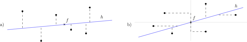
Figure 2: a) If $0\leq\alpha\leq\varphi_{v}$ then all points move vertically to $h$. b) if $\varphi_{v}<\alpha\leq\frac{\pi}{4}$ then some points move vertically to $h$, some other points move horizontally, and the rest of the points move directly to $f$.

Because of Lemma 2.3, the travel time $d_{h}(p,f)$ between a demand point $p$ and facility $f$ simplifies to:

$$\min\left\{\begin{array}[]{l}\|p-f\|_{1},\\ \|p-p^{\prime}\|_{1}+\frac{\|p^{\prime}-f\|_{2}}{v},\\ \|p-p^{\prime\prime}\|_{1}+\frac{\|p^{\prime\prime}-f\|_{2}}{v}\end{array}\right.$$ (7)

Given a solution $(f,h)$ to the FFL-problem, we can always partition the set $S$ of demand points into there sets $S_{1}:=S_{1}(f,h)$, $S_{2}:=S_{2}(f,h)$, and $S_{3}:=S_{3}(f,h)$ as follows. Set $S_{1}$ contains the points $p\in S$ such that $x_{p}\leq x_{f}$ and $y_{p}\geq y_{f}$ and the points $q\in S$ such that $x_{q}\geq x_{f}$ and $y_{q}\leq y_{f}$. Set $S_{2}$ contains the points $p\in S$ such that $x_{p}<x_{f}$ and $p$ is either on or below $h$, and the points $q\in S$ such that $x_{q}>x_{f}$ and $q$ is either on or above $h$. Set $S_{3}$ is equal to $S\setminus(S_{1}\cup S_{2})$. It is straightforward to obtain what follows (refer to Fig. 3).

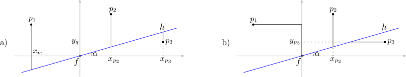
Figure 3: Points $p_{1}$, $p_{2}$, and $p_{3}$ belong to $S_{1}$, $S_{2}$, and $S_{3}$, respectively. In case a) we have $0\leq\alpha\leq\varphi_{v}$. In case b) we have $\varphi_{v}<\alpha\leq\frac{\pi}{4}$.

If $0\leq\alpha\leq\varphi_{v}$ then $d_{h}(p,f)$ is equal to:

$$\left\{\begin{array}[]{rr}|y_{p}-y_{f}|+|x_{p}-x_{f}|\tan\alpha+\frac{|x_{p}-x_{f}|}{\cos\alpha\cdot v}&\text{ if }p\in S_{1}\\ |y_{p}-y_{f}|-|x_{p}-x_{f}|\tan\alpha+\frac{|x_{p}-x_{f}|}{\cos\alpha\cdot v}&\text{ if }p\in S_{2}\\ -|y_{p}-y_{f}|+|x_{p}-x_{f}|\tan\alpha+\frac{|x_{p}-x_{f}|}{\cos\alpha\cdot v}&\text{ if }p\in S_{3}\end{array}\right.$$

and the objective function $\Phi(f,h)$ equals:

$$\sum_{p\in S_{1}}w_{p}|y_{p}-y_{f}|+\sum_{p\in S_{2}}w_{p}|y_{p}-y_{f}|-\sum_{p\in S_{3}}w_{p}|y_{p}-y_{f}|+$$

$$\tan\alpha\left(\sum_{p\in S_{1}}w_{p}|x_{p}-x_{f}|-\sum_{p\in S_{2}}w_{p}|x_{p}-x_{f}|+\sum_{p\in S_{3}}w_{p}|x_{p}-x_{f}|\right)+$$

$$\frac{1}{\cos\alpha\cdot v}\sum_{p\in S}w_{p}|x_{p}-x_{f}|$$ (8)

Otherwise, if $\varphi_{v}<\alpha\leq\frac{\pi}{4}$, then $d_{h}(p,f)$ is equal to:

$$\left\{\begin{array}[]{cr}|x_{p}-x_{f}|+|y_{p}-y_{f}|&\text{ if }p\in S_{1}\\ |y_{p}-y_{f}|-|x_{p}-x_{f}|\tan\alpha+\frac{|x_{p}-x_{f}|}{\cos\alpha\cdot v}&\text{ if }p\in S_{2}\\ |x_{p}-x_{f}|-|y_{p}-y_{f}|\cot\alpha+\frac{|y_{p}-y_{f}|}{\sin\alpha\cdot v}&\text{ if }p\in S_{3}\end{array}\right.$$

and $\Phi(f,h)$ equals:

$$\sum_{p\in S_{1}}w_{p}\left(|x_{p}-x_{f}|+|y_{p}-y_{f}|\right)+\sum_{p\in S_{2}}w_{p}|y_{p}-y_{f}|+\sum_{p\in S_{3}}w_{p}|x_{p}-x_{f}|+$$

$$\left(\frac{1}{\cos\alpha\cdot v}-\tan\alpha\right)\sum_{p\in S_{2}}w_{p}|x_{p}-x_{f}|+\left(\frac{1}{\sin\alpha\cdot v}-\cot\alpha\right)\sum_{p\in S_{3}}w_{p}|y_{p}-y_{f}|$$ (9)

3 Reducing the search space

Let $G$ be the grid defined by the set of all axis-parallel lines passing through the elements of $S$.

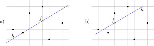
Figure 4: a) Lemma 3.1 (a). b) Lemma 3.1 (b)

Lemma 3.1

There always exists an optimal solution $(f,h)$ to the FFL-problem satisfying one of the next statements: $(a)$ $h$ contains a point of $S$ and $f$ is on a line of grid $G$, and $(b)$ $f$ is a vertex of grid $G$. Refer to Fig. 4.

• Let $(f,h)$ be an optimal solution of the FFL-problem satisfying neither condition (a) nor condition (b). Using local linear perturbations, we will transform $(f,h)$ into other optimal solution that satisfies at least one of these conditions.

  Assume first the case where $\varphi_{v}<\alpha\leq\frac{\pi}{4}$. Let $\delta_{1}\geq 0$ (resp. $\delta_{2}\geq 0$) be the smallest value such that if we translate both $f$ and $h$ with vector $(-\delta_{1},0)$ (resp. $(\delta_{2},0)$) then $f$ belongs to a vertical line of $G$ or $h$ contains a point of $S$. Given $\varepsilon\in[-\delta_{1},\delta_{2}]$, let $f_{\varepsilon}$ and $h_{\varepsilon}$ be $f$ and $h$ translated with vector $(\varepsilon,0)$, respectively. Using Lemma 2.3, we partition $S$ into four sets $Z_{1}$, $Z_{2}$, $Z_{3}$, and $Z_{4}$ as follows. Set $Z_{1}$ (resp. $Z_{2}$) contains the demand points doing a rightwards (resp. leftwards) movement to reach $h$. Set $Z_{3}$ (resp. $Z_{4}$) contains the demand points doing only a downwards (resp. upwards) movement to reach $h$. Observe that:

  $$d_{h_{\varepsilon}}(p,f_{\varepsilon})-d_{h}(p,f)=\left\{\begin{array}[]{cr}\varepsilon&\text{ if }p\in Z_{1}\\ -\varepsilon&\text{ if }p\in Z_{2}\\ \varepsilon\cdot c_{\alpha}&\text{ if }p\in Z_{3}\\ -\varepsilon\cdot c_{\alpha}&\text{ if }p\in Z_{4}\end{array}\right.$$

  where $c_{\alpha}=\tan\alpha-\frac{1}{\cos\alpha\cdot v}$. Let $W_{i}$ denote $\sum_{p\in Z_{i}}w_{p}$, $(i=1,2,3,4)$. Thus, for any $\varepsilon\in[-\delta_{1},\delta_{2}]$, the variation of objective function when we translate both $f$ and $h$ with vector $(\varepsilon,0)$ is the following:

  $$\Phi(f_{\varepsilon},h_{\varepsilon})-\Phi(f,h) = \sum_{p\in S}w_{p}\cdot\left(d_{h_{\varepsilon}}(p,f_{\varepsilon})-d_{h}(p,f)\right)$$

  $$= \sum_{p\in Z_{1}}w_{p}\varepsilon+\sum_{p\in Z_{2}}w_{p}(-\varepsilon)+$$

  $$\sum_{p\in Z_{3}}w_{p}(\varepsilon c_{\alpha})+\sum_{p\in Z_{4}}w_{p}\left(-\varepsilon c_{\alpha}\right)$$

  $$= \varepsilon\left(W_{1}-W_{2}+c_{\alpha}(W_{3}-W_{4})\right)$$

  Since $(f,h)$ is optimal we must have $\Phi(f_{\varepsilon},h_{\varepsilon})-\Phi(f,h)\geq 0$ for all $\varepsilon\in[-\delta_{1},\delta_{2}]$. It implies $W_{1}-W_{2}+c_{\alpha}(W_{3}-W_{4})=0$ and $\Phi(f_{\varepsilon},h_{\varepsilon})=\Phi(f,h)$ for all $\varepsilon\in[-\delta_{1},\delta_{2}]$. Therefore, by translating both $f$ and $h$ with vector either $(-\delta_{1},0)$ or $(\delta_{2},0)$, we ensure that $f$ is on a vertical line of $G$ or $h$ passes through a point of $S$, or both conditions. If it holds only that $f$ is on a vertical line of $G$, then we repeat the same operation in the vertical direction in order to ensure that $f$ is on a horizontal line of $G$ or $h$ passes through a point of $S$, and condition (a) or condition (b) holds. Otherwise, if it holds only that $h$ passes through a point of $S$, then it is straightforward to prove, by using similar arguments, that $f$ can be translated along $h$ in order to ensure that $f$ belongs to a line of $G$, that is either vertical or horizontal, and condition (a) holds. In fact, for some demand point $p$ of $S$, $f$ will coincide with the point in which $p$ enters $h$, that is, $p^{\prime}$ or $p^{\prime\prime}$.

  In the case where $0\leq\alpha\leq\varphi_{v}$ every demand point $p$ moves vertically to $h$ (Lemma 2.3), and we can proceed as follows by using arguments similar to the above ones. We first translate vertically both $f$ and $h$ with the same vector in order to ensure that $h$ contains a point of $S$. After that, $f$ is translated along $h$ if necessary in order to $f$ belongs to a vertical line of $G$ and condition (a) holds. The lemma thus follows.  ${\square}$

Corollary 3.2

If $\alpha\leq\varphi_{v}$ then there is an optimal solution satisfying Lemma 3.1 $(a)$.

4 The algorithm to solve the FFL-problem

Theorem 4.1

The FFL-problem can be solved in $O(n^{3})$ time.

• We find an optimal solution by solving two cases separately. The first case is when solution satisfies Lemma 3.1 (a), and the second case is when solution satisfies Lemma 3.1 (b).

  In order to solve the first case we find for each demand point $p$ and each line $\ell$ of $G$ an optimal angle $\alpha$ such that $\Phi(f_{\alpha},h_{\alpha})$ is minimized, where $h_{\alpha}$ is the line passing through $p$ whose angle with respect to the positive direction of the $x$-axis is equal to $\alpha$, and $f_{\alpha}$ is the intersection point between $\ell$ and $h_{\alpha}$. Assume w.l.o.g. that $\ell$ is vertical and $p$ is located to the left of $\ell$. It is easy to observe from equations (8) and (9) that for any $\alpha\in[0,\frac{\pi}{4}]$ the expression of $\Phi(f_{\alpha},h_{\alpha})$ has the form $b_{1}+b_{2}\tan\alpha+b_{3}\cot\alpha+\frac{b_{4}}{\cos\alpha}+\frac{b_{5}}{\sin\alpha}$, where $b_{1},b_{2},b_{3},b_{4},b_{5}$ are constants. Furthermore, if we progressively increase the value of $\alpha$ from $0$ to $\frac{\pi}{4}$, that expression changes whenever sets $S_{1}$, $S_{2}$, and $S_{3}$ change, that is, when $h_{\alpha}$ crosses a demand point, $f_{\alpha}$ crosses a horizontal line of $G$, or $\alpha=\varphi_{v}$. Then consider the sequence $0=\alpha_{0}<\alpha_{1}<\dots<\alpha_{m}=\frac{\pi}{4}$ of $m+1=O(n)$ angles, where each angle $\alpha_{i}$ $(1\leq i<m)$ is such that either $h_{\alpha_{i}}$ contains a demand point, $f_{\alpha_{i}}$ belongs to a horizontal line of grid $G$, or $\alpha_{i}=\varphi_{v}$. Notice then that the expression of $\Phi(f_{\alpha},h_{\alpha})$ is the same for all $\alpha\in[\alpha_{i},\alpha_{i+1}]$ $(0\leq i<m)$. If we preprocess the demand points $S$ by constructing the dual arrangement of $S$ [20], such a sequence can be obtained in $O(n)$ time by using both the Zone Theorem [20] and the order of the demand points with respect to the $y$-coordinate. Observe that if for a value of $i$ we know the expression of $\Phi(f_{\alpha},h_{\alpha})$ in the interval $[\alpha_{i},\alpha_{i+1}]$, then $\Phi(f_{\alpha},h_{\alpha})$ can be minimized in constant time in that interval. Furthermore, if $h_{\alpha_{i+1}}$ contains a demand point or $f_{\alpha_{i+1}}$ belongs to a horizontal line of $G$, then the expression of $\Phi(f_{\alpha},h_{\alpha})$ in the interval $[\alpha_{i+1},\alpha_{i+2}]$ can be obtained in constant time from the expression of $\Phi(f_{\alpha},h_{\alpha})$ in the interval $[\alpha_{i},\alpha_{i+1}]$. It is easy to see now that $\Phi(f_{\alpha},h_{\alpha})$, $0\leq\alpha\leq\frac{\pi}{4}$, can be minimized in $O(n)$ time by minimizing $\Phi(f_{\alpha},h_{\alpha})$ in $[\alpha_{i},\alpha_{i+1}]$ for $i=0,1,\dots,m-1$. Since there are $n$ demand points and $G$ has $2n$ lines, then an overall $O(n^{3})$-time algorithm is obtained.

  We can proceed similarly in order to solve the second case. We find an optimal solution $(u,h)$ for each vertex $u$ of the grid $G$ as follows. Let $u$ be a vertex of $G$. Given an angle $\alpha$, let $h_{\alpha}$ be the line passing through $u$, whose angle with respect to the positive direction of the $x$-axis is equal to $\alpha$. Then, by Corollary 3.2, we look for an angle $\alpha\in(\varphi_{v},\frac{\pi}{4}]$ such that the objective function $\Phi(u,h_{\alpha})$ is minimized. It follows from equation (9) that the expression of $\Phi(u,h_{\alpha})$ has the form $c_{1}+c_{2}\tan\alpha+c_{3}\cot\alpha+\frac{c_{4}}{\cos\alpha}+\frac{c_{5}}{\sin\alpha}$ for any $\alpha\in(\varphi_{v},\frac{\pi}{4}]$, where $c_{1},\ldots,c_{5}$ are constants. If we progressively increase $\alpha$ from $\varphi_{v}$ to $\frac{\pi}{4}$ the expression of $\Phi(u,h_{\alpha})$ keeps unchanged as long as $h_{\alpha}$ does not cross a demand point. The sorted sequence of values of $\alpha$ in which it happens can be obtained in linear time by using duality [20]. That sequence of values induces a partition of the interval $(\varphi_{v},\frac{\pi}{4}]$ into intervals where in each of them the expression of $\Phi(u,h_{\alpha})$ is constant. We can now continue as was done above to solve the first case. Since $G$ has $O(n^{2})$ vertices then an overall $O(n^{3})$-time algorithm is thus obtained. The result thus follows.  ${\square}$

5 A refinement of the algorithm

Theorem 4.1 shows an algorithm that solves the FFL-problem by dividing the search of optimal solutions into two steps. It first looks in $O(n^{3})$ time for an optimal solution that satisfies Lemma 3.1 (a), and after that looks within the same time complexity for an optimal solution satisfying Lemma 3.1 (b). In the following we show that for “reasonable” values of speed $v$ we can simplify the algorithm of Theorem 4.1 by finding only optimal solutions that hold Lemma 3.1 (a). We will use the next technical lemma.

Lemma 5.1

Let $a$, $b$, $c$, and $v>\frac{3\sqrt{2}}{4}$ be non-negative constants and $F:(0,\frac{\pi}{2})\rightarrow\mathbb{R}$ be a function so that

$$F(x)=a\left(\frac{1-v\sin x}{\cos x}\right)+b\left(\frac{1-v\cos x}{\sin x}\right)+c$$

for all $x\in(0,\frac{\pi}{2})$. Then next statements are true:

• If $a=0$ and $b=0$ then $F$ is constant.

• If $a>0$ and $b=0$ then $F$ is monotone decreasing.

• If $a=0$ and $b>0$ then $F$ is monotone increasing.

• If $a>0$ and $b>0$ then $F$ has no minima.

• Statement (a) is immediate. Let $F^{\prime}$ be the first derivative of $F$ and observe that:

  $$F^{\prime}(x)=a\left(\frac{\sin x-v}{\cos^{2}x}\right)+b\left(\frac{v-\cos x}{\sin^{2}x}\right)$$

  If $a>0$ and $b=0$ then $\lim_{x\rightarrow 0^{+}}F(x)=a$, $\lim_{x\rightarrow\frac{\pi}{2}^{-}}F(x)=-\infty$, and equation $F^{\prime}(x)=0$ has no solution in $(0,\frac{\pi}{2})$ because $v>1$. Therefore, $F(x)$ is a monotone decreasing function and statement (b) thus holds.

  If $a=0$ and $b>0$ then $\lim_{x\rightarrow 0^{+}}F(x)=-\infty$, $\lim_{x\rightarrow\frac{\pi}{2}^{-}}F(x)=b$, and equation $F^{\prime}(x)=0$ has no solution in $(0,\frac{\pi}{2})$ because $v>1$. Therefore, $F(x)$ is a monotone increasing function and statement (c) thus holds.

  Consider $a>0$ and $b>0$. Since $\lim_{x\rightarrow 0^{+}}F(x)=\lim_{x\rightarrow\frac{\pi}{2}^{-}}F(x)=-\infty$ it suffices to prove that equation $F^{\prime}(x)=0$ has only one solution which must be a global maximum of $F$. Equation $F^{\prime}(x)=0$ is equivalent to equation

  $$G(x):=\frac{\sin^{2}x(v-\sin x)}{\cos^{2}x(v-\cos x)}=\frac{b}{a}$$

  We will prove that equation $G^{\prime}(x)=0$ has no solution in $(0,\frac{\pi}{2})$, which implies that equation $G(x)=\frac{b}{a}$ has a unique solution in $(0,\frac{\pi}{2})$ because $\lim_{x\rightarrow 0^{+}}G(x)=0<\frac{b}{a}<+\infty=\lim_{x\rightarrow\frac{\pi}{2}^{-}}G(x)$. This will complete the proof.

  It is straightforward to see that equation $G^{\prime}(x)=0$ is equivalent to equation $H(x):=0$, where $H(x)$ is equal to:

  $$2(v-\sin x)(v-\cos x)+\sin x\cos x(1-v(\sin x+\cos x))$$

  Consider the function $I:(0,\frac{\pi}{2})\rightarrow\mathbb{R}$ so that

  $$I(x)=2(v-\sin x)(v-\cos x)+\sin x\cos x(1-\sqrt{2}v)$$

  for all $x\in(0,\frac{\pi}{2})$. Since $\sin x+\cos x\leq\sqrt{2}$ and $\sin x\cos x>0$ for all $x\in(0,\frac{\pi}{2})$, we have $H(x)\geq I(x)$ for all $x\in(0,\frac{\pi}{2})$. We now show that the minimum of $I(x)$ in $(0,\frac{\pi}{2})$ is greater than zero, implying equation $H(x)=0$ has no solution.

  $$I^{\prime}(x) = 2(-\cos x(v-\cos x)+\sin x(v-\sin x))+$$

  $$(1-\sqrt{2}v)(\cos^{2}x-\sin^{2}x)$$

  $$= 2(\cos x-\sin x)(\cos x+\sin x-v)+$$

  $$(1-\sqrt{2}v)(\cos x-\sin x)(\cos x+\sin x)$$

  $$= (\cos x-\sin x)\left((3-\sqrt{2}v)(\sin x+\cos x)-2v\right)$$

  If $3-\sqrt{2}v<0$ then there is no $x\in(0,\frac{\pi}{2})$ such that $(3-\sqrt{2}v)(\sin x+\cos x)-2v=0$ because $\sin x+\cos x$ is positive for all $x\in(0,\frac{\pi}{2})$. Suppose $3-\sqrt{2}v\geq 0$. Then we have:

  $$(3-\sqrt{2}v)(\sin x+\cos x)-2v \leq (3-\sqrt{2}v)\sqrt{2}-2v$$

  $$= 3\sqrt{2}-4v$$

  $$< 0$$

  and thus there is no $x\in(0,\frac{\pi}{2})$ such that $(3-\sqrt{2}v)(\sin x+\cos x)-2v=0$. Therefore, $I^{\prime}(x)=0$ if and only if $\cos x-\sin x=0$, that is, $x=\frac{\pi}{4}$. Let us prove that $I(\frac{\pi}{4})>0$.

  $$I\left(\frac{\pi}{4}\right)=2\left(v-\frac{\sqrt{2}}{2}\right)^{2}+\frac{1}{2}\left(1-\sqrt{2}v\right)=2v^{2}-\frac{5\sqrt{2}}{2}v+\frac{3}{2}$$

  The roots of polynomial $P(x):=2x^{2}-\frac{5\sqrt{2}}{2}x+\frac{3}{2}$ are respectively equal to $\frac{1}{4}\left(\frac{5\sqrt{2}}{2}-\frac{\sqrt{2}}{2}\right)$ and $\frac{1}{4}\left(\frac{5\sqrt{2}}{2}+\frac{\sqrt{2}}{2}\right)=\frac{3\sqrt{2}}{4}$. Then we conclude that $P(v)=I\left(\frac{\pi}{4}\right)>0$ because the main coefficient of $P(x)$ is positive, $\frac{3\sqrt{2}}{4}$ is the greatest root of $P(x)$, and $v>\frac{3\sqrt{2}}{4}$. Since $\lim_{x\rightarrow 0^{+}}I(x)=\lim_{x\rightarrow\frac{\pi}{2}^{-}}I(x)=2v(v-1)>0$ and $I(x)>0$ at the unique extreme point $x=\frac{\pi}{4}$, then $I(x)>0$ for all $x\in(0,\frac{\pi}{2})$. Therefore, $H(x)>0$ for all $x\in(0,\frac{\pi}{2})$, equation $G^{\prime}(x)$ has no solution in $(0,\frac{\pi}{2})$, and then $F(x)$ has only one extreme point in $(0,\frac{\pi}{2})$ which is a global maximum. The lemma follows.  ${\square}$

Lemma 5.2

If speed $v$ is greater than $\frac{3\sqrt{2}}{4}\approx 1.060660172$, then there always exists an optimal solution $(f,h)$ to the FFL-problem satisfying Lemma 3.1 $(a)$, that is, $h$ contains a point of $S$ and $f$ is on a line of grid $G$.

• It suffices to show that for every solution $(f,h)$, there exists another solution $(f^{\prime},h^{\prime})$ satisfying Lemma 3.1 (a) and $\Phi(f^{\prime},h^{\prime})\leq\Phi(f,h)$. The proof is as follows.

  Let $(f,h)$ be a solution of the FFL-problem so that $h$ contains no demand point. Assume here angle $\alpha$ satisfies $0\leq\alpha<\frac{\pi}{2}$. If $\alpha$ is such that $0\leq\alpha\leq\varphi_{v}$, then the result follows from Corollary 3.2. Therefore, assume $\varphi_{v}<\alpha\leq\frac{\pi}{2}$. We proceed to prove that there exists another solution $(f^{\prime},h^{\prime})$ such that $h^{\prime}$ contains a demand point and $\Phi(f^{\prime},h^{\prime})\leq\Phi(f,h)$. Consider the sets $S_{2}=S_{2}(f,h)$ and $S_{3}=S_{3}(f,h)$ as defined before.

  Given an angle $\beta\in[\varphi_{v},\frac{\pi}{2})$, let $h_{\beta}$ be the line passing through $f$ so that the angle between $h_{\beta}$ and the positive direction of the $x$-axis is equal to $\beta$. Observe then by equation (9) that $\Phi(f,h)$ is equal to:

  $$\Phi(f,h_{\alpha})=a\left(\frac{1-v\sin\alpha}{\cos\alpha}\right)+b\left(\frac{1-v\cos\alpha}{\sin\alpha}\right)+c$$

  where $a$, $b$, and $c$ are non-negative constants that depend on the coordinates of the demand points and the speed $v$. Then we can argue what follows by both noting that $a>0$ (resp. $b>0$) if and only if $S_{2}$ (resp. $S_{3}$) is not empty and using Lemma 5.1.

  We can rotate $h$ with center $f$ by either increasing or decreasing $\alpha$ to the value $\alpha^{\prime}\in[\varphi_{v},\frac{\pi}{2})$ in such a way solution $(f,h_{\alpha^{\prime}})$ is obtained, where either $\alpha^{\prime}=\varphi_{v}$ or $h_{\alpha^{\prime}}$ contains a demand point of $S_{2}\cup S_{3}$, and $\Phi(f,h_{\alpha^{\prime}})\leq\Phi(f,h)$. If $\alpha^{\prime}=\varphi_{v}$ then the result follows from Corollary 3.2. Otherwise, if $h_{\alpha^{\prime}}$ contains a demand point of $S_{2}\cup S_{3}$, then $(f^{\prime},h^{\prime})=(f,h_{\alpha^{\prime}})$ is the desired solution, and to finalize the proof, we translate $f^{\prime}$ along $h^{\prime}$, if necessary, as was done in the proof of Lemma 3.1, in order to ensure $f^{\prime}$ belongs to a line of grid $G$. The result thus follows.  ${\square}$

6 Examples

In Fig. 5 and Fig. 6 we show the same example, consisting of nine demand points $p_{1},p_{2},\ldots,p_{9}$. Each demand point is represented by a solid dot, and labeled with a triple, the first two components are the coordinates and the third component is its weight. Facility point $f$ is represented by a cross. In both examples optimal solutions satisfy Lemma 3.1 (a), that is, highway contains a demand point and facility point belongs to a line of grid $G$. As expected, when we increase the highway’s speed from the example in Fig. 5 to the one in Fig. 6, the shortest paths to the facility point change according to the claims of Lemma 2.3.

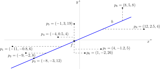
Figure 5: The highway contains a demand point and facility point belongs to a line of grid $G$. Some points perform an horizontal movement to reach the highway.

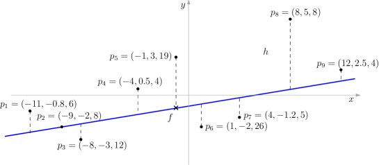
Figure 6: The highway contains a demand point and facility point belongs to a line of grid $G$. All points perform only a vertical movement to reach the highway.

In Fig. 5 speed $v$ is equal to $1.2$ and highway $h$ of the optimal solution contains point $p_{3}$, facility point $f=(-1,-0.14335)$ is on the vertical line passing through $p_{5}$, and there are some demand points moving horizontally to reach facility point $f$. The value of the objective function $\Phi(f,h)$ is equal to $525.83$.

In Fig. 6 speed $v$ is equal to $1.5$, highway $h$ of the optimal solution contains point $p_{2}$, facility $f=(-1,-0.7758)$ is on the vertical line containing $p_{5}$, and all demand points move vertically only to reach the highway. Since speed is greater than speed in Fig. 5, the value of the objective function $\Phi(f,h)$ reduces to $471.55$.

In Fig. 7 we present a different example consisting of nine demand points $p_{1},\ldots,p_{9}$, with the aim of showing the existence of configurations for which optimal solutions satisfy only Lemma 3.1 (b). In this example speed $v$ is equal to $1.04<\frac{3\sqrt{2}}{4}$. Highway $h$ of the optimal solution contains no demand point and facility $f=(0,0)$ is on a vertex of grid $G$, in fact, it is located on both the horizontal line through $p_{7}$ and the vertical line through $p_{6}$. The value of $\Phi(f,h)$ is equal to $336.2$.

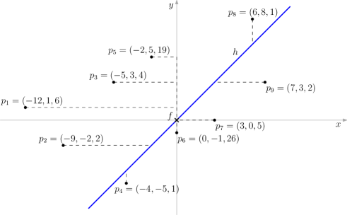
Figure 7: The highway contains no demand point and facility point is a vertex of grid $G$.

7 Conclusions and further research

We have solved in $O(n^{3})$ time the problem of locating at the same time a facility point and a freeway of variable length, among a set of demand points, in order to minimize the total weighted travel time from the demand points to the facility. Some examples are presented to show that there exist optimal solutions corresponding to each type of solutions that our algorithm considers.

A natural restriction to be considered in further research of this problem is to upper bound the length of the highway, that is, to consider that highway has fixed length. In this case, there also exist optimal solutions in which the facility point belongs to the highway. This was in fact showed in Proposition 2.2 because in the proof we did not change the lenght of the highway. It is not hard to see that when the highway’s length is fixed, the shortest paths from the demand points to the facility point can be discretized as follows. If $0\leq\alpha\leq\varphi_{v}$, then we distinguish three regions $R_{1}$, $R_{2}$, and $R_{3}$ as depicted in Fig. 8 a). Points belonging to $R_{1}\cup R_{3}$ move to the nearest endpoint of $h$, and points of $R_{2}$ move vertically to $h$. Otherwise, if $\varphi_{v}<\alpha\leq\frac{\pi}{4}$, then eight regions $R_{1},\ldots,R_{8}$ can be identified as shown in Fig. 8 b). Points of $R_{1}\cup R_{2}$ move to the nearest endpoint of $h$, points of $R_{3}\cup R_{4}$ move directly to $f$, points of $R_{5}\cup R_{6}$ move horizontally to $h$, and points of $R_{7}\cup R_{8}$ move vertically to $h$.

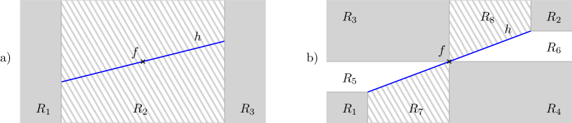
Figure 8: Discretization when the highway’s length is fixed.

We believe that with the above discretization, the search space of optimal solutions can be simplified by using a similar (and more detailed) statement as Lemma 3.1. This will permit to obtain an algorithm similar to the one presented in Theorem 4.1.

Other variant to be considered in further research is the problem of locating at the same time the facility point and a turnpike of variable length. This will extend [12, 14].

References

- [1] M. Abellanas, F. Hurtado, C. Icking, R. Klein, E. Langetepe, L. Ma, B. Palop, and V. Sacristán. Voronoi diagram for services neighboring a highway. Information Processing Letters, 86:283–288, 2003.
- [2] P. K. Agarwal and M. Sharir. Davenport-Schinzel Sequences and their Geometric Applications. Cambridge University Press, New York, NY, USA, 2010.
- [3] H-K. Ahn, H. Alt, T. Asano, S. W. Bae, P. Brass, O. Cheong, C. Knauer, H-S. Na, C S. Shin, and A. Wolff. Constructing optimal highways. In Proc. 13th Australasian symposium on Theory of computing, volume 65 of CATS ’07, pages 7–14, Darlinghurst, Australia, 2007.
- [4] O. Aichholzer, F. Aurenhammer, and B. Palop. Quickest paths, straight skeletons, and the city Voronoi diagram. In Proc. 18th Annu. ACM Sympos. Comput. Geom., pages 151–159, 2002.
- [5] G. Aloupis, J. Cardinal, S. Collette, F. Hurtado, S. Langerman, J. O’Rourke, and B. Palop. Highway hull revisited. Comput. Geom. Theory Appl., 43:115–130, February 2010.
- [6] S. W. Bae, M. Korman, and T. Tokuyama. All farthest neighbors in the presence of highways and obstacles. In Proc. 3rd International Workshop on Algorithms and Computation, WALCOM’09, pages 71–82, Berlin, Heidelberg, 2009. Springer-Verlag.
- [7] J. Brimberg, H. T. Kakhki, and G. O. Wesolowsky. Location among regions with varying norms. Annals of Operations Research, 122(1):87–102, 2003.
- [8] J. Brimberg, H. T. Kakhki, G. O. Wesolowsky, and M. Unzverszty. Locating a single facility in the plane in the presence of a bounded region and different norms. Journal of the Operations Research Society of Japan, 48(2):135–147, 2005.
- [9] J. Cardinal, S. Collette, F. Hurtado, S. Langerman, and B. Palop. Optimal location of transportation devices. Comput. Geom. Theory Appl., 41:219–229, 2008.
- [10] E. Carrizosa and A. M. Rodríguez-Chía. Weber problems with alternative transportation systems. European Journal of Operational Research, 97(1):87–93, 1997.
- [11] J. M. Díaz-Báñez, M. Korman, P. Pérez-Lantero, and I. Ventura. The 1-center and 1-highway problem. In Proc. 14th Spanish Meeting on Computational Geometry, pages 193–196, Alcalá de Henares, Spain, June 2011.
- [12] J. M. Díaz-Báñez, M. Korman, P. Pérez-Lantero, and I. Ventura. Locating a service facility and a rapid transit line. In Proc. 14th Spanish Meeting on Computational Geometry, pages 189–192, Alcalá de Henares, Spain, June 2011.
- [13] J. M. Díaz-Báñez, J. A. Mesa, and A. Schöbel. Continuous location of dimensional structures. European Journal of Operational Research, 152(1):22–44, 2004.
- [14] I. Espejo and A. M. Rodríguez-Chía. Simultaneous location of a service facility and a rapid transit line. Comput. Oper. Res., 38:525–538, 2011.
- [15] M. Gugat and B. Pfeiffer. Weber problems with mixed distances and regional demand. Mathematical Methods of Operations Research, 66(3):419–449, 2007.
- [16] P-H. Huang, Y. T. Tsai, and C. Y. Tang. A fast algorithm for the alpha-connected two-center decision problem. Inf. Process. Lett., 85:205–210, 2003.
- [17] M. Korman. Theory and Applications of Geometric Optimization Problems in Rectilinear Metric Spaces. PhD thesis, Tohoku University, 2009. Committee: T. Nishizeki, A. Shinohara, A. Shioura and T. Tokuyama.
- [18] M. Korman and T. Tokuyama. Optimal insertion of a segment highway in a city metric. In Proc. 14th annual international conference on Computing and Combinatorics, COCOON’08, pages 611–620, Berlin, Heidelberg, 2008.
- [19] M.-C. Körner and A. Schöbel. Weber problems with high-speed lines. TOP, 18(1):223–241, 2010.
- [20] Joseph O’Rourke. Computational Geometry in C. Cambridge University Press, New York, NY, USA, 2nd edition, 1998.
- [21] B. Pfeiffer and K. Klamroth. A unified model for weber problems with continuous and network distances. Comput. Oper. Res., 35(2):312–326, 2008.