Large-Scale Structure with Gravitational Waves I: Galaxy Clustering

Abstract

Observed angular positions and redshifts of large-scale structure tracers such as galaxies are affected by gravitational waves through volume distortion and magnification effects. Thus, a gravitational wave background can in principle be probed through clustering statistics of large-scale structure. We calculate the observed angular clustering of galaxies in the presence of a gravitational wave background at linear order including all relativistic effects. For a scale-invariant spectrum of gravitational waves, the effects are most significant at the smallest multipoles ($2\leq\ell\leq 5$), but typically suppressed by six or more orders of magnitude with respect to scalar contributions for currently allowed amplitudes of the inflationary gravitational wave background. We also discuss the most relevant second-order terms, corresponding to the distortion of tracer correlation functions by gravitational waves. These provide a natural application of the approach recently developed in Schmidt and Jeong (2012a).

I Introduction

The origin of the initial perturbations which gave rise to the structure in the Universe is one of the most profound questions in cosmology. Currently, the most popular scenario is inflation Starobinsky (1980); Guth (1981), a phase of accelerating expansion in the very early Universe which produced seed perturbations as quantum fluctuations frozen after exiting the horizon. One of the key predictions of inflation is a potentially observable background of stochastic gravitational waves (GW). A detection of a GW background would allow for a determination of the energy scale of inflation, and pose a significant challenge to competing scenarios for the origin of the initial perturbations.

The polarization of the cosmic microwave background (CMB) is widely considered to be the most promising probe of the primordial GW background in the near future Seljak and Zaldarriaga (1997); Kamionkowski et al. (1997). However, given the profound impact of a detection, it is worth studying complementary observational techniques, in order to be able to provide independent confirmation of a positive result. The study of the effect of GW on large-scale structure observables has a long history. Linder (1988) considered the distortion of galaxy correlation functions and derived an upper limit on the GW background. Bar-Kana (1996) studied the apparent proper motion of distant objects induced by GW (see also Book and Flanagan (2011); Bharadwaj and Guha Sarkar (2009)). More recently, Book et al. (2011a) have studied the prospects for using gravitational lensing of the CMB for this purpose. At redshifts of order $10-200$, the 21cm HI emission from the dark ages has been proposed as a potentially extremely sensitive probe of a GW background Masui and Pen (2010); Book et al. (2011b). Due to its three-dimensional nature and observable structure on much smaller scales, the 21cm emission should in principle be able to probe GW amplitudes orders of magnitude smaller than the CMB. The shear, measured through correlations of galaxy ellipticities, has also been studied as avenue for detecting a GW background Dodelson et al. (2003); Dodelson (2010), though these authors have concluded that this measurement will likely not be competitive with the CMB (see also Schmidt and Jeong (2012b)).

The goal of this paper, and its companion Schmidt and Jeong (2012b), is to systematically and rigorously derive the GW effects on large-scale structure observables. While we restrict ourselves to a linear treatment in the tensor perturbations, we strive to keep the results as general as possible otherwise. This paper deals with observed densities of large-scale structure tracers, which have so far not been investigated in the context of two-point statistics as a probe of GW. The companion paper deals with shear (as measured from, e.g., galaxy ellipticities).

Since there is no 3-scalar that can be constructed from tensor perturbations at linear order without making reference to some external (3-)vector or tensor, the “intrinsic” density of tracers, i.e. the density that would be measured by a local comoving observer, is not affected by tensor modes at linear order. Thus, the impact of tensor perturbations is exclusively due to projection effects which can be derived in analogy to Yoo et al. (2009); Challinor and Lewis (2011); Bonvin and Durrer (2011); Jeong et al. (2012) using the geodesic equation. The main observable we consider is the angular power spectrum $C(l)$ of tracers. Since the GW effects are most important on the very largest scales, the 3D power spectrum $P(k)$ is not a meaningful quantity for this purpose.

Note that in contrast, the shear is itself a tensorial quantity, and thus there is a possible “intrinsic” contribution correlated with the GW background, analogous to the intrinsic alignment effect present for scalar perturbations. This issue, which has not been investigated before, is the topic of the companion paper Schmidt and Jeong (2012b).

As emphasized by Kaiser and Jaffe (1997), there are some key differences in how tensor perturbations affect photon geodesics as opposed to scalar perturbations: scalar modes which are transverse to the line of sight lead to a significantly amplified coherent deflection, whereas the same does not happen for tensor modes as they themselves propagate at the speed of light. Furthermore, while scalar modes grow (in the matter-dominated era), tensor modes redshift away. Thus, the intuition that transverse modes at lower redshifts contribute most of the projection (lensing) effects does not hold anymore for tensor modes. Rather, the GW contribution to the clustering of LSS tracers is dominated by contributions close to the time of emission, and time-derivatives of the perturbations are (at least) as relevant as spatial derivatives.

The outline of the paper is as follows. We introduce our notation and conventions in § II. § III presents the geodesic equation for a tensor mode and the derivation of the tensor mode contributions to the observed galaxy density, including the magnification bias contribution. The galaxy angular power spectrum is discussed in § IV. We also highlight the differences to the scalar case in this calculation. § V deals with the relevant higher order terms neglected in § III. We conclude in § VI. The appendix contains details on some aspects of the calculation.

II Preliminaries

We begin by introducing our convention for metric and tensor perturbations and some notation. For simplicity, we restrict ourselves to a spatially flat FRW background, and consider only tensor (gravitational wave) modes in the main part of the paper. The perturbed metric is then given by

$$ds^{2}=a^{2}(\eta)\left[-d\eta^{2}+\left(\delta_{ij}+h_{ij}\right)dx^{i}dx^{j}\right],$$ (1)

where $h_{ij}$ is a metric perturbation which is transverse and traceless:

$$h^{i}_{\;i}=0=(h_{ik})^{,i}.$$ (2)

In order to simplify the analysis, we shall also consider the conformal metric,

$$d\bar{s}^{2}=-d\eta^{2}+\left(\delta_{ij}+h_{ij}\right)dx^{i}dx^{j},$$ (3)

where $\eta$ denotes the conformal time, for our analysis of the light deflection.

We then decompose $h_{ij}$ into Fourier modes of two polarization states,

$$h_{ij}(\mathbf{k},\eta)=\> e^{+}_{ij}(\hat{\mathbf{k}})h^{+}(\mathbf{k},\eta)+e^{\times}_{ij}(\hat{\mathbf{k}})h^{\times}(\mathbf{k},\eta),$$ (4)

where $e^{s}_{ij}(\hat{\mathbf{k}})$, $s=+,\times$, are transverse (with respect to $\hat{\mathbf{k}}$) and traceless polarization tensors normalized through $e^{s}_{ij}e^{s^{\prime}\>ij}=2\delta^{ss^{\prime}}$. We assume both polarizations to be independent and to have equal power spectra:

$$\langle h_{s}(\mathbf{k},\eta)h_{s^{\prime}}(\mathbf{k}^{\prime},\eta^{\prime})\rangle=\> (2\pi)^{3}\delta_{D}(\mathbf{k}-\mathbf{k}^{\prime})\delta_{ss^{\prime}}\frac{1}{4}P_{T}(k,\eta,\eta^{\prime}).$$ (5)

Here, $\eta$ denotes conformal time, and the unequal-time power spectrum is given by

$$P_{T}(k,\eta,\eta^{\prime})=\> T_{T}(k,\eta)T_{T}(k,\eta^{\prime})P_{T0}(k),$$ (6)

where $T_{T}(k,\eta)$ is the tensor transfer function, and the primordial tensor power spectrum is specified through an amplitude $\Delta_{T}^{2}$ and an index $n_{T}$ via

$$P_{T0}(k)=\> 2\pi^{2}\,k^{-3}\left(\frac{k}{k_{0}}\right)^{n_{T}}\Delta_{T}^{2}.$$ (7)

Following WMAP convention Komatsu et al. (2011), we choose $k_{0}=0.002\>{\rm Mpc}^{-1}$ as pivot scale. Throughout, we will assume a scalar-to-tensor ratio of $r=0.2$ at $k_{0}$ (consistent with the 95% confidence level WMAP bound), which together with our fiducial cosmology determines $\Delta_{T}^{2}$. The tensor index is chosen to follow the inflationary consistency relation, $n_{T}=-r/8=-0.0025$. For the expansion history, we assume a flat $\Lambda$CDM cosmology with $h=0.72$ and $\Omega_{m}=0.28$. Contributions from scalar perturbations are evaluated using a spectral index of $n_{s}=0.958$ and power spectrum normalization at $z=0$ of $\sigma_{8}=0.8$.

From Eq. (4) and Eq. (5), we easily obtain

$$\langle h_{ij}(\mathbf{k},\eta)h_{kl}(\mathbf{k}^{\prime},\eta^{\prime})\rangle=\> (2\pi)^{3}\delta_{D}(\mathbf{k}-\mathbf{k}^{\prime})$$ (8)

$$\times\left[e^{+}_{ij}(\hat{\mathbf{k}})e^{+}_{kl}(\hat{\mathbf{k}})+e^{\times}_{ij}(\hat{\mathbf{k}})e^{\times}_{kl}(\hat{\mathbf{k}})\right]$$

$$\times\frac{1}{4}P_{T}(k,\eta,\eta^{\prime})$$

$$\langle h_{ij}(\mathbf{k},\eta)h^{ij}(\mathbf{k}^{\prime},\eta^{\prime})\rangle=\> (2\pi)^{3}\delta_{D}(\mathbf{k}-\mathbf{k}^{\prime})P_{T}(k,\eta,\eta^{\prime}).$$

Long after recombination, the transverse anisotropic stress which sources gravitational waves becomes negligible, and the tensor modes propagate as free waves. During matter-domination, the tensor transfer function then simply becomes

$$T_{T}(k,\eta)=3\frac{j_{1}(k\eta)}{k\eta},$$ (9)

which however is still valid to a high degree of accuracy during the current epoch of acceleration. We will use Eq. (9) throughout.

III Tensor contributions to the observed galaxy density

In this section we derive the GW contribution to the observed density of tracers, including the magnification bias effect. We follow the notation in Jeong et al. (2012) (see also Schmidt and Jeong (2012a)) which is summarized in their Sec. II A. The zero-th order photon geodesic in conformal coordinates [Eq. (3)] is simply

$$\bar{x}^{\mu}(\chi)=\left(\eta_{0}-\chi,\hat{\mathbf{n}}\chi\right),$$ (10)

where the comoving distance $\chi$ along the geodesic serves as affine parameter, with $\chi=0$ corresponding to the observer’s location. Here and throughout, $\hat{\mathbf{n}}$ denotes the unit vector in the direction of the observed position of the source ($\hat{\tilde{n}}$ in Jeong et al. (2012)). Hence,

$$\frac{d\bar{x}^{\mu}}{d\chi}=(-1,\hat{\mathbf{n}}).$$ (11)

In the following, $\tilde{z}$ will stand for the observed redshift of the source, and $\tilde{\chi}\equiv\bar{\chi}(\tilde{z})$ is the conformal distance corresponding to that redshift when evaluating the distance-redshift relation $\bar{\chi}(z)$ in the background.

We decompose vectors into transverse and longitudinal parts with respect to the line-of-sight,

$$X_{\parallel}\equiv\> \hat{n}_{i}\,X^{i}$$

$$X_{\perp}\equiv\> X^{i}-\hat{n}^{i}\,\hat{n}_{j}\,X^{j},$$ (12)

and correspondingly define longitudinal and transverse derivatives through

$$\partial_{\parallel}\equiv\> \hat{n}^{i}\,\partial_{i}$$

$$\partial_{\perp}^{i}\equiv\> \partial^{i}-\hat{n}^{i}\partial_{\parallel}.$$ (13)

Finally, we define

$$\nabla^{2}_{\perp}\equiv\partial_{\perp i}\partial_{\perp}^{i}=\nabla^{2}-\partial_{\parallel}^{2}-\frac{2}{\tilde{\chi}}\partial_{\parallel},$$ (14)

and make use of

$$\partial_{\parallel}\hat{\tilde{n}}^{i}=\> \hat{\tilde{n}}^{i}\partial_{\perp i}=0.$$ (15)

III.1 Photon geodesics with a tensor mode

We now briefly outline the derivation of the displacements $\Delta x^{i}$ of the true emission point from the observationally inferred position. This is a special case of the derivation in App. B of Schmidt and Jeong (2012a), to which the reader is referred for more details. We parameterize the linear order deviation of the photon geodesic as

$$\frac{dx^{\mu}}{d\chi}=(-1+\delta\nu,\hat{\mathbf{n}}+\delta\mathbf{e}).$$ (16)

The initial conditions for integrating the geodesic equation are set by demanding that the components of the photon momentum measured in a locally orthonormal frame at the observer’s location match $\hat{\mathbf{n}}$. For that, we construct an orthonormal tetrad $(e^{a})_{\mu}$ ($a=0,1,2,3$) carried by an observer so that at the observer’s location

$$g^{\mu\nu}(e^{a})_{\mu}(e^{b})_{\nu}=\eta^{ab}.$$ (17)

Then, the photon four-momentum measured by the observer is given by

$$\left(1,\hat{n}^{i}\right)=\left((e^{0})_{\mu},(e^{i})_{\mu}\right)\frac{dx^{\mu}}{d\chi}.$$ (18)

A detailed calculation is presented in appendix B of Schmidt and Jeong (2012a). Using that the four-velocity of comoving observers is given by $u^{\mu}=a^{-1}(1,0,0,0)$, this leads to

$$\delta\nu(\chi=0)=\> 0$$

$$\delta e^{i}(\chi=0)=\> -\frac{1}{2}(h^{i}_{\;j})_{o}\>\hat{n}^{j}.$$ (19)

Here and throughout, a subscript $o$ indicates that the quantity is evaluated at the observer’s location. The corresponding initial condition for the geodesic equation for comoving observers with general metric is presented in Eq. (B11) of Schmidt and Jeong (2012a). In case of scalar perturbations, including $\delta e^{i}(\chi=0)$ is important to ensure gauge-invariant expressions Jeong et al. (2012). While there is no gauge ambiguity in tensor modes, we will show that the observer term is numerically important for the quadrupole of the observed galaxy density. The redshift perturbation is related to the shift in the frequency through

$$\delta z(\tilde{\chi})=-\delta\nu=\frac{1}{2}\int_{0}^{\tilde{\chi}}h_{\parallel}^{\prime}d\chi,$$ (20)

where we have defined

$$h_{\parallel}\equiv h_{ij}\,\hat{n}^{i}\hat{n}^{j}.$$ (21)

Here and hereafter, a prime denotes a derivative with respect to conformal time, if not used for distinguishing different variables. The distinction between the two should be clear from the context. The redshift of the photon along the perturbed geodesic is given by $1+z(\chi)=[1+\delta z(\chi)]/a(x^{0}(\chi))$. Requiring that the redshift at emission equals $\tilde{z}$ yields an equation for the first-order perturbation to the affine parameter at emission $\chi_{e}$ Jeong et al. (2012),

$$\chi_{e}=\> \tilde{\chi}+\delta\chi$$

$$\delta\chi=\> \delta x^{0}-\frac{1+\tilde{z}}{H(\tilde{z})}\delta z,$$ (22)

where $\delta x^{0}$ is the perturbation to the 0th component of the geodesic evaluated at $\chi=\tilde{\chi}$. We now relate the observed position $\tilde{\mathbf{x}}$, inferred assuming the unperturbed geodesic $\bar{x}^{\mu}$, and the true position $\mathbf{x}$ through (see Fig. 1 in Jeong et al. (2012))

$$\Delta\mathbf{x}\equiv\mathbf{x}-\tilde{\mathbf{x}}=\delta x(\tilde{\chi})+\hat{\mathbf{n}}\delta\chi,$$ (23)

where $\delta x(\tilde{\chi})$ is the spatial perturbation to the geodesic evaluated at $\chi=\tilde{\chi}$. We can then decompose the displacement $\Delta\mathbf{x}$ into perpendicular and longitudinal parts,

$$\Delta x_{\parallel}=\> \delta x^{i}\hat{n}_{i}+\delta x^{0}-\frac{1+\tilde{z}}{H(\tilde{z})}\delta z$$ (24)

$$\Delta x_{\perp}=\> \Delta x^{i}-\hat{n}^{i}\Delta x_{\parallel}.$$ (25)

Explicitly,

$$\Delta x_{\parallel}=\> -\frac{1}{2}\int_{0}^{\tilde{\chi}}d\chi\>h_{\parallel}-\frac{1+\tilde{z}}{2H(\tilde{z})}\int_{0}^{\tilde{\chi}}d\chi\>h_{\parallel}^{\prime}$$ (26)

and

$$\Delta x_{\perp}^{i}=\> \frac{1}{2}\tilde{\chi}\left[\left(h_{ij}\right)_{o}\hat{n}^{j}-\left(h_{\parallel}\right)_{o}\hat{n}^{i}\right]$$

$$+\int_{0}^{\tilde{\chi}}d\chi\left\{\frac{\tilde{\chi}-\chi}{2}\partial_{\perp}^{i}h_{\parallel}+\frac{\tilde{\chi}}{\chi}\left(h_{\parallel}\hat{n}^{i}-h_{ij}\hat{n}^{j}\right)\right\}.$$ (27)

Note that Eqs. (26)–(27) can be obtained directly from Eqs. (43)–(47) in Schmidt and Jeong (2012a) (with $\delta z=\Delta\ln a$) by setting $A=B=v=0$, or, alternatively, from the corresponding Eqs. (38)–(39) in Jeong et al. (2012) by restricting to a transverse-traceless metric perturbation and setting $E_{\parallel}=h_{\parallel}/2$.

In the following, we will further need the convergence $\hat{\kappa}$, defined through (see App. A)

$$\hat{\kappa}\equiv\> -\frac{1}{2}\partial_{\perp i}\Delta x_{\perp}^{i}$$

$$=\> \frac{5}{4}h_{\parallel o}-\frac{1}{2}h_{\parallel}-\frac{1}{2}\int_{0}^{\tilde{\chi}}d\chi\Big{[}h_{\parallel}^{\prime}+\frac{3}{\chi}h_{\parallel}\Big{]}$$

$$-\frac{1}{4}\nabla^{2}_{\Omega}\int_{0}^{\tilde{\chi}}d\chi\frac{\tilde{\chi}-\chi}{\tilde{\chi}\>\chi}h_{\parallel}.$$ (28)

Here $\nabla^{2}_{\Omega}=\chi^{2}\nabla_{\perp}^{2}$ is the Laplacian on the sphere. Also, we will use

$$\partial_{\tilde{\chi}}\Delta x_{\parallel}=\> -\frac{1}{2}h_{\parallel}-\frac{1+\tilde{z}}{2H(\tilde{z})}h_{\parallel}^{\prime}$$

$$-\frac{H(\tilde{z})}{2}\frac{\partial}{\partial\tilde{z}}\left[\frac{1+\tilde{z}}{H(\tilde{z})}\right]\int_{0}^{\tilde{\chi}}d\chi h_{\parallel}^{\prime},$$ (29)

where we have used $d\tilde{\chi}=d\tilde{z}/H(\tilde{z})$. While $\hat{\kappa}$ is the usual coordinate convergence, $\partial_{\tilde{\chi}}\Delta x_{\parallel}$ is the distortion of the volume along the line of sight and can thus be seen as a “radial convergence”.

III.2 Observed galaxy density

The observed comoving number density of galaxies $a^{3}\tilde{n}_{g}$ is related to the true comoving number density $a^{3}n_{g}$ through

$$a^{3}(\tilde{z})\tilde{n}_{g}(\tilde{\bm{x}},\tilde{z})=\left(1+\frac{1}{2}\delta g^{\mu}_{\;\mu}\right)a^{3}(\bar{z})n_{g}(\bm{x},\bar{z})\left(1+\frac{\partial\Delta x^{i}}{\partial\tilde{x}^{i}}\right).$$ (30)

The first term in brackets comes from the covariant volume factor $\sqrt{|g|}$ and is equal to unity, since for transverse-traceless metric perturbations $\delta g^{\mu}_{\;\mu}=0$ at linear order. The factor $a^{3}(\bar{z})n_{g}(\mathbf{x},\bar{z})$ is the true comoving number density at the point of emission, which we expand as

$$a^{3}(\bar{z})n_{g}(\mathbf{x},\bar{z})=a^{3}(\bar{z})\bar{n}_{g}(\bar{z})\>[1+\delta_{g}(\mathbf{x},\bar{z})],$$ (31)

by defining the intrinsic perturbations to the comoving number density $\delta_{g}$. $\bar{z}$ is the redshift that would be measured for the source in an unperturbed universe, and is related to $\tilde{z}$ through

$$1+\tilde{z}=(1+\bar{z})(1+\delta z).$$ (32)

Note that, when inserting Eq. (31) into Eq. (30), the distinction between $\mathbf{x}$ and $\tilde{\mathbf{x}}$ in the argument of $\delta_{g}$ is second order if we regard intrinsic galaxy density perturbations as first order, which we will do in this section. The relevant additional terms will be studied in § V. Finally, $1+\partial_{i}\Delta x^{i}$ is the volume distortion due to gravitational waves, which as derived in Jeong et al. (2012) becomes

$$\frac{\partial\Delta x^{i}}{\partial\tilde{x}^{i}}=\partial_{\tilde{\chi}}\Delta x_{\parallel}+\frac{2\Delta x_{\parallel}}{\tilde{\chi}}-2\hat{\kappa}.$$ (33)

Thus, gravitational waves affect the observed density of galaxies through a volume distortion effect, and by perturbing their redshifts so that we compare the measured galaxy density $\tilde{n}_{g}$ to the “wrong” background density $\bar{n}_{g}(\tilde{z})$. The latter effect is quantified by the parameter

$$b_{e}\equiv\frac{d\ln(a^{3}\bar{n}_{g})}{d\ln a}\Big{|}_{\!\tilde{z}}=-(1+\tilde{z})\frac{d\ln(a^{3}\bar{n}_{g})}{dz}\Big{|}_{\!\tilde{z}}.$$ (34)

Note that this parameter can be measured for a given galaxy sample, provided the redshift-dependence of the selection function is understood.

We can now summarize the tensor contributions to the observed galaxy density perturbation as

$$\tilde{\delta}_{gT}(\tilde{\bm{x}},\tilde{z})=\> b_{e}\delta z-2\hat{\kappa}-\frac{1}{\tilde{\chi}}\left[\int_{0}^{\tilde{\chi}}d\chi h_{\parallel}+\frac{1+\tilde{z}}{H(\tilde{z})}\int_{0}^{\tilde{\chi}}d\chi h_{\parallel}^{\prime}\right]$$

$$- \frac{1}{2}h_{\parallel}-\frac{1+\tilde{z}}{2H(\tilde{z})}h_{\parallel}^{\prime}-\frac{H(\tilde{z})}{2}\frac{\partial}{\partial\tilde{z}}\left[\frac{1+\tilde{z}}{H(\tilde{z})}\right]\int_{0}^{\tilde{\chi}}d\chi h_{\parallel}^{\prime}.$$ (35)

Here, the subscript $T$ denotes tensor contributions, and we have assumed that the intrinsic density perturbation $\delta_{g}$ does not correlate with the tensor modes (following the arguments in § I). Note that $h_{ij}$ only enters through $h_{\parallel}$. This has to be the case, since the galaxy density is a scalar quantity and $h_{\parallel}$ is the only non-trivial scalar linear in $h_{ij}$. The latter also implies that tensor modes do not contribute to the monopole and dipole of the galaxy density.

III.3 Magnification bias

In the last section, we have assumed that all galaxies are included in the sample. In reality, most large-volume surveys are limited in flux. A cut on observed flux induces additional fluctuations in the galaxy density, since perturbations to the photon geodesic (e.g., gravitational lensing) modify the observed flux of a given source. The magnification $\mathcal{M}$ can be derived as the perturbation to the angular diameter distance squared (Jeong et al. (2012), with $\delta\mathcal{M}_{\rm there}=\mathcal{M}_{\rm here}$),

$$1+\mathcal{M}\equiv\frac{\bar{D}^{2}_{A}(\tilde{z})}{D^{2}_{A}},$$ (36)

where $D_{A}$ is the true angular diameter distance to the source while $\bar{D}_{A}(z)$ is the background angular diameter distance-redshift relation. Alternatively, one can use the standard ruler approach of Schmidt and Jeong (2012a), which for a metric of the form Eq. (1) yields (see Eq. (105) in Schmidt and Jeong (2012a), where we set $d\ln r_{0}/d\ln a=0$ neglecting the higher order effect of an evolving number count slope)

$$\mathcal{M}_{T}=-2\delta z+\frac{1}{2}h_{\parallel}-\frac{2\Delta x_{\parallel}}{\tilde{\chi}}+2\hat{\kappa}.$$ (37)

We then parametrize the effect on the observed galaxy density through a parameter $\mathcal{Q}$,

$$\tilde{\delta}_{gT}=\tilde{\delta}_{gT}(\mathrm{no~{}magn.})+\mathcal{Q}\mathcal{M}_{T}.$$ (38)

For a purely flux-limited survey, $\mathcal{Q}=-d\ln\bar{n}_{g}/d\ln f_{\rm cut}$, where $f_{\rm cut}$ is the flux cut. More generally, $\mathcal{Q}$ can also receive a contribution from a size cut Schmidt et al. (2009).

III.4 Summary of tensor contributions

Combining the result of the last two sections, we obtain the following expression for the linear-order tensor contributions to the observed galaxy density:

$$\tilde{\delta}_{gT}=\> (b_{e}-2\mathcal{Q})\delta z-2(1-\mathcal{Q})\hat{\kappa}-\frac{1-\mathcal{Q}}{2}h_{\parallel}-\frac{1+\tilde{z}}{2H(\tilde{z})}h_{\parallel}^{\prime}$$

$$-\frac{1-\mathcal{Q}}{\tilde{\chi}}\left[\int_{0}^{\tilde{\chi}}d\chi h_{\parallel}+\frac{1+\tilde{z}}{H(\tilde{z})}\int_{0}^{\tilde{\chi}}d\chi h_{\parallel}^{\prime}\right]$$

$$-\frac{H(\tilde{z})}{2}\frac{\partial}{\partial\tilde{z}}\left[\frac{1+\tilde{z}}{H(\tilde{z})}\right]\int_{0}^{\tilde{\chi}}d\chi h_{\parallel}^{\prime}.$$ (39)

For later convenience, we reorder the terms as follows:

$$\tilde{\delta}_{gT}=\> f_{\tilde{\chi}}h_{\parallel}+f_{\tilde{\chi}}^{\prime}h_{\parallel}^{\prime}+f\int\frac{d\chi}{\chi}h_{\parallel}+\tilde{f}\int\frac{d\chi}{\tilde{\chi}}h_{\parallel}$$ (40)

$$+f^{\prime}\int d\chi\>h_{\parallel}^{\prime}+f_{\kappa}\nabla^{2}_{\Omega}\int d\chi\frac{\tilde{\chi}-\chi}{\chi\,\tilde{\chi}}h_{\parallel}+f_{o}\,h_{\parallel o}.$$

Here, all terms outside integrals (without subscript $o$) are evaluated at $\tilde{\chi}$, and the integrals go from 0 to $\tilde{\chi}$. The coefficients are given by

$$f_{\tilde{\chi}}=\> -\frac{1}{2}(\mathcal{Q}-1)$$ (41)

$$f^{\prime}_{\tilde{\chi}}=\> -\frac{1+\tilde{z}}{2H}$$

$$f=\> -3(\mathcal{Q}-1)$$

$$\tilde{f}=\> \mathcal{Q}-1$$

$$f^{\prime}=\> \frac{1}{2}\left(b_{e}-1-2\mathcal{Q}+(1+\tilde{z})\frac{dH/d\tilde{z}}{H}\right)-(\mathcal{Q}-1)$$

$$+(\mathcal{Q}-1)\frac{1+\tilde{z}}{H\tilde{\chi}}$$

$$f_{\kappa}=\> -\frac{1}{2}(\mathcal{Q}-1)$$

$$f_{o}=\> \frac{5}{2}(\mathcal{Q}-1).$$

IV Observed galaxy power spectrum

IV.1 Angular power spectrum

Consider a galaxy sample with a redshift distribution $dN/dz$, normalized to unity in redshift. Then, the projected galaxy overdensity as a function of position on the sky is given by

$$\Delta_{g}(\hat{\mathbf{n}})=\int_{0}^{\infty}d\tilde{z}\frac{dN}{d\tilde{z}}\tilde{\delta}_{g}(\bar{\chi}(\tilde{z})\hat{\mathbf{n}};\tilde{z}),$$ (42)

We will assume that the quantities $b_{e},\>\mathcal{Q}$ describing the galaxy sample are independent of redshift for simplicity. We can then write the multipole coefficients of the galaxy density as

$$a^{g}_{lm}=\> \int d^{2}\hat{\mathbf{n}}\>Y^{*}_{lm}(\hat{\mathbf{n}})\Delta_{g}(\hat{\mathbf{n}}).$$ (43)

We can write all individual contributions to Eq. (39) as

$$A(\hat{\mathbf{n}},\tilde{\chi})=\> \int_{0}^{\tilde{\chi}}d\chi\>W_{A}(\chi,\tilde{\chi})h_{\parallel}(\chi\hat{\mathbf{n}},\chi)$$

$$=\> \int_{0}^{\tilde{\chi}}d\chi\>W_{A}(\chi,\tilde{\chi})$$

$$\times\int\frac{d^{3}\mathbf{k}}{(2\pi)^{3}}e^{i\mathbf{k}\cdot\hat{\mathbf{n}}\chi}\hat{n}^{i}\hat{n}^{j}h_{ij}(\mathbf{k},\eta_{0}-\chi).$$ (44)

Note that terms involving $h_{\parallel}^{\prime}$ can be brought into the form $A(\hat{\mathbf{n}})$ by including $d\ln T_{T}(k,\eta)/d\eta$ in $W_{A}(\chi)$. The observer term $5h_{\parallel o}/3$ contained in $\hat{\kappa}$ can similarly be written with $W_{A}(\chi)=5/3\,\delta_{D}(\chi)$. We will deal with that term specifically in § IV.2. By changing the order of integration, we can then write the contribution to the projected galaxy overdensity as

$$A(\hat{\mathbf{n}})=\> \int_{0}^{\infty}d\tilde{z}\frac{dN}{d\tilde{z}}A(\hat{\mathbf{n}},\tilde{\chi})=\int_{0}^{\infty}d\chi\>\mathcal{W}_{A}(\chi)h_{\parallel}(\chi\hat{\mathbf{n}},\chi)$$

$$\mathcal{W}_{A}(\chi)\equiv\> \int_{z(\chi)}^{\infty}d\tilde{z}\frac{dN}{d\tilde{z}}W_{A}\left(\chi,\bar{\chi}(\tilde{z})\right).$$ (45)

Note that if $W_{A}=\delta_{D}(\chi-\tilde{\chi})$, $\mathcal{W}_{A}(\chi)=(HdN/dz)|_{z(\chi)}$. We now consider the contribution of a single plane wave tensor perturbation with $\mathbf{k}$-vector aligned with the $z$-direction. Then,

$$\hat{n}^{i}\hat{n}^{j}h_{ij}(\mathbf{k},\eta)=\> \sin^{2}\theta\left[\cos 2\phi\>h^{+}(\mathbf{k},\eta)+\sin 2\phi\>h^{\times}(\mathbf{k},\eta)\right]$$

$$=\> \sin^{2}\theta\left[e^{i2\phi}h_{1}+e^{-i2\phi}h_{2}\right],$$ (46)

where

$$h_{1,2}\equiv\> \frac{1}{2}(h^{+}\pm ih^{\times}).$$ (47)

Note that the power spectra of these circular polarization staters are $P_{h_{1}h_{2}}=P_{h_{2}h_{2}}=P_{T}/8$, while $P_{h_{1}h_{2}}=0$. Let us denote as $A(\hat{\mathbf{n}},\mathbf{k})$ the contribution to $A(\hat{\mathbf{n}})$ from this plane-wave tensor perturbation. We have

$$A(\hat{\mathbf{n}},\mathbf{k})=\> \int d\chi\>\mathcal{W}_{A}(\chi)e^{ik\chi\mu}(1-\mu^{2})$$ (48)

$$\times\left[e^{2i\phi}h_{1}(\mathbf{k},\eta_{0}-\chi)+e^{-2i\phi}h_{2}(\mathbf{k},\eta_{0}-\chi)\right]$$

where $\mu=\cos\theta$ is the cosine of the angle between $\hat{\mathbf{n}}$ and $\hat{\mathbf{k}}$. Note the $e^{\pm 2i\phi}$ factors which are the key difference to the case of scalar perturbations. The multipole coefficients of $A$ are then obtained as follows:

$$a^{A}_{lm}=\int\frac{d^{3}\mathbf{k}}{(2\pi)^{3}}a^{A}_{lm}(\mathbf{k}),$$ (49)

$$a^{A}_{lm}(\mathbf{k})=\> \int d^{2}\hat{\mathbf{n}}\>Y^{*}_{lm}(\hat{\mathbf{n}})A(\hat{\mathbf{n}})$$

$$=\> \int d\chi\>\mathcal{W}_{A}(\chi)\int d^{2}\hat{\mathbf{n}}\>Y^{*}_{lm}(\mu,\phi)e^{ik\chi\mu}(1-\mu^{2})\left[e^{2i\phi}h_{1}(\mathbf{k},\eta_{0}-\chi)+e^{-2i\phi}h_{2}(\mathbf{k},\eta_{0}-\chi)\right].$$ (50)

We now use the relation (see App. A1 in Schmidt and Jeong (2012a))

$$\int d\Omega\>Y^{*}_{lm}(1-\mu^{2})e^{\pm i2\phi}e^{ix\mu}=\> -\sqrt{4\pi(2l+1)}\sqrt{\frac{(l+2)!}{(l-2)!}}\,i^{l}\frac{j_{l}(x)}{x^{2}}\delta_{m\pm 2},$$ (51)

which yields

$$a^{A}_{lm}(\mathbf{k})=\> -\sqrt{\frac{2l+1}{4\pi}\frac{(l+2)!}{(l-2)!}}(4\pi)i^{l}\int d\chi\>\mathcal{W}_{A}(\chi)\left[h_{1}(\mathbf{k},\eta_{0}-\chi)\delta_{m2}+h_{2}(\mathbf{k},\eta_{0}-\chi)\delta_{m-2}\right]\frac{j_{l}(k\chi)}{(k\chi)^{2}}.$$ (52)

Further, we can use the properties of the spherical harmonics to obtain

$$a_{lm}[\nabla^{2}_{\Omega}A]=-l(l+1)a^{A}_{lm},$$ (53)

which we will use to evaluate the convergence contribution. Using the definition of the angular power spectrum, we can now easily write down the cross-correlation between two different projections $A,\,B$ of $h_{\parallel}$ (App. A1 in Schmidt and Jeong (2012a)):

$$C^{AB}_{l}\equiv\> \frac{1}{2l+1}\sum_{m}\mbox{Re}\langle a^{A*}_{lm}a^{B}_{lm}\rangle$$

$$=\> \frac{1}{2\pi}\frac{(l+2)!}{(l-2)!}\int k^{2}dk\>P_{T0}(k)F_{l}^{A}(k)F_{l}^{B}(k)$$ (54)

$$F_{l}^{X}(k)\equiv\> \int d\chi\>\mathcal{W}_{X}(\chi)T_{T}(k,\eta_{0}-\chi)\frac{j_{l}(k\chi)}{(k\chi)^{2}}.$$ (55)

It is then straightforward to evaluate auto- and cross-correlations of the observed angular correlation of galaxies, neglecting the contribution of the term $h_{\parallel o}$ for the moment (see § IV.2). In particular, if we want to evaluate the total tensor contribution to the angular (auto-)power spectrum of galaxies, we set $W_{A}=W_{B}=W_{g}$, where

$$W_{g}(\chi)=\> f_{\tilde{\chi}}\delta_{D}(\chi-\tilde{\chi})+\frac{d\ln T_{T}}{d\eta}\Big{|}_{\eta_{0}-\chi}\left(f^{\prime}_{\tilde{\chi}}\delta_{D}(\chi-\tilde{\chi})+f^{\prime}\right)$$

$$+f\frac{1}{\chi}+\tilde{f}\frac{1}{\tilde{\chi}}-f_{\kappa}\>l(l+1)\frac{\tilde{\chi}-\chi}{\chi\,\tilde{\chi}},$$ (56)

and the coefficients are defined in Eq. (41). Note that the divergent pieces $\propto\chi^{-1}$ cancel for $l=2$:

$$f-6f_{\kappa}=0,$$ (57)

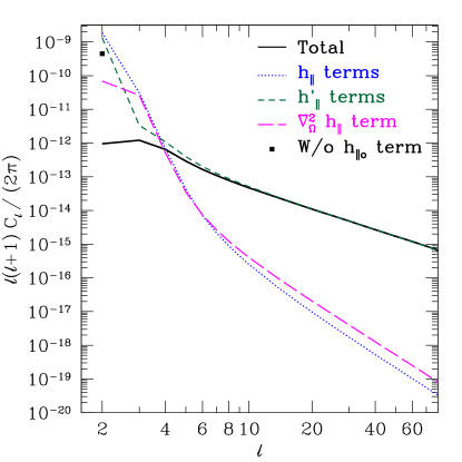
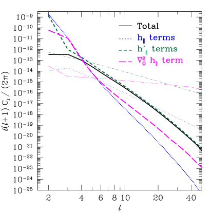
while for $l\geq 3$ the Bessel function in Eq. (55) ensures that all terms are regular. Fig. 1 shows numerical results for a galaxy sample with a sharp (observed) redshift of $\tilde{z}=2$, and for $b_{e}=2.5,\;Q=1.5$. The colored lines indicate the separate contributions proportional to projections of $h_{\parallel}$, $h^{\prime}_{\parallel}$, and $\nabla_{\Omega}^{2}h_{\parallel}$. While for $l\lesssim 4$ all terms contribute significantly, the $h^{\prime}_{\parallel}$ contribution dominates at higher $l$. This contribution is the same as the GW effect $\delta_{h}^{s}$ explored in Bharadwaj and Guha Sarkar (2009). We will return to this in § IV.4. Note that the total contribution (black solid line) is significantly smaller than the individual contributions for $l=2,\,3$. We will discuss this in the next section.

Figure 1: Contributions to the observed galaxy angular power spectrum from inflationary gravitational waves, for a sharp source galaxy redshift of $\tilde{z}=2$, and using the tensor mode power spectrum defined in § II. The black solid line shows the total contribution, while the colored lines show contributions proportional to line-of-sight integrals of $h_{\parallel}$ (blue dotted), $h_{\parallel}^{\prime}$ (green short-dashed) and $\nabla_{\Omega}^{2}h_{\parallel}$ (magenta long-dashed). Here, we have assumed $b_{e}=2.5,\;Q=1.5$. The black square at $l=2$ indicates the result for $l=2$ if the observer term is neglected (see § IV.2).

IV.2 Quadrupole

Fig. 1 shows that the individual tensor contributions to the observed angular power spectrum increase rapidly towards small $l$, while the total contribution is much smaller. These cancellations are essentially a consequence of causality, which demands that the observed clustering of galaxies cannot depend on tensor modes that are super-horizon today.

In particular, it is important to take into account the last term in Eq. (40), which quantifies the shearing of the observer’s coordinate system by the gravitational waves. We refer to this as the observer term. Since $h_{ij}(o)$ is a constant (transverse-traceless) tensor, this term only contributes to the quadrupole $l=2$. Specifically, we have an additional contribution to Eq. (55) for galaxies,

$$F_{l=2}^{g}(k)\to\> F_{l=2}^{g}(k)+F_{2}^{g,o}(k)$$

$$F_{2}^{g,o}(k)=\> f_{o}\lim_{\chi\to 0}T_{T}(k,\eta_{0}-\chi)\frac{j_{2}(k\chi)}{(k\chi)^{2}}$$

$$=\> \frac{1}{15}f_{o}\,T_{T}(k,\eta_{0}).$$ (58)

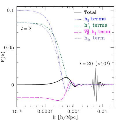
The solid black line in Fig. 1 includes this term, while the black square indicates the value of $C_{l=2}$ we would obtain without this term. Neglecting the observer term results in an overestimation of the tensor contribution to the galaxy quadrupole by three orders of magnitude. The reason for this significant effect becomes clear when considering the contributions to $F^{g}_{l=2}$ as function of $k$ (Fig. 2). The individual contributions to $F^{g}_{l}$ approach a constant as $k\to 0$, while the sum goes to zero for $k/H_{0}\lesssim 1$, as demanded by causality. When neglecting the observer term (light blue in Fig. 2) on the other hand, a residual constant contribution to $F^{g}_{l=2}$ remains for $k\to 0$, which together with the steeply falling tensor power spectrum leads to a significant overestimation of the quadrupole.

Figure 2: Contributions to the kernel $F_{l}(k)$ for $l=2$ (thick) and $l=20$ (thin, only total contribution shown, scaled by $10^{4}$), for a sharp source redshift $\tilde{z}=2$ and the same parameters as in Fig. 1. Note that the separate contributions have non-zero weight for $k\to 0$, while the total $F^{g}_{l}$ (black solid) is only non-zero for $k\gtrsim 10^{-4}\>h/{\rm Mpc}$, as required by causality.

IV.3 Limber approximation

In the context of angular galaxy clustering, one often uses the Limber approximation Limber (1954) which significantly simplifies the calculation of $C^{g}_{l}$. The underlying assumption is that the dominant contribution to the angular clustering comes from galaxy pairs that are at similar distances along the line of sight. It is instructive to consider this approximation in the context of tensor modes. Since the Limber approximation works best for a broad redshift distribution, we will here consider a redshift distribution roughly as expected for the Large Synoptic Survey Telescope (LSST LSS ),

$$\frac{dN}{dz}\propto z^{2}\exp\left[-\left(\frac{z}{z_{0}}\right)^{\beta}\right],$$ (59)

with $z_{0}=0.15$ and $\beta=0.73$, yielding a mean redshift of 1.2.

The Limber approximation can formally be applied by using

$$\frac{2}{\pi}\int k^{2}dk\,F(k,\chi)\,j_{l}(k\chi)j_{l}(k\chi^{\prime})\approx\frac{F\left(\frac{l+1/2}{\chi},\chi\right)}{\chi^{2}}\delta_{D}(\chi-\chi^{\prime}).$$ (60)

In the usual application to scalars, the functions of $k,\,\chi$ involved (apart from the Bessel functions) are smooth and positive, whereas for tensor modes, the transfer function is oscillatory. Performing the $k$ and then one of the $\chi$ integrals in Eq. (54) leads to

$$C^{AB}_{l}\approx\> \frac{(l+2)!}{(l-2)!}\frac{1}{(l+1/2)^{4}}\frac{1}{4}\int\frac{d\chi}{\chi^{2}}P_{T0}\left(\frac{l+1/2}{\chi}\right)$$ (61)

$$\hskip 19.91684pt\times\mathcal{W}_{A}(\chi)\mathcal{W}_{B}(\chi)\left[T_{T}\left((l+1/2)\frac{\eta_{0}-\chi}{\chi}\right)\right]^{2}.$$

Here we have used that $T_{T}$ is only a function of $k\eta$. Note that for $l\gg 1$, the prefactor approaches $1/4$. Given that $P_{T0}\propto k^{-3+n_{T}}$, we immediately see that the Limber approximation predicts $C^{g}_{l}\propto l^{-3+n_{T}}$ for large $l$, if $\mathcal{W}_{A,B}$ are $l$-independent.

Fig. 3 shows the different contributions to $C^{g}_{l}$ (as in Fig. 1) for the redshift distribution Eq. (59) using the full calculation (thick lines) and using the Limber approximation (thin lines). Clearly, the Limber approximation predicts the wrong $l$-scaling of all terms, and we do not see any improvement in the approximation for high $l$ as in the scalar case. Thus, the Limber approximation is not applicable for calculating the tensor contribution to the angular galaxy power spectrum at any $\ell$. There are two reasons for this. First, the tensor mode power spectrum is falling as $\sim k^{-3}$, so that the assumption that pairs of comparable line-of-sight distance dominate because they have the smallest separation does not hold. Second, tensor modes oscillate and decay towards late times (while scalar modes grow), so that the contributions to $C^{g}_{l}$ are concentrated at large scales and high redshifts near the source.

Figure 3: Contributions of tensor modes to the angular galaxy power spectrum for a broad redshift distribution (Eq. (59)) expected for LSST, separated into different contributions as in Fig. 1 (again using $b_{e}=2.5,\;Q=1.5$). The thick lines show the exact calculation, while the thin lines show the Limber approximation using Eq. (61).

IV.4 Dependence on galaxy sample

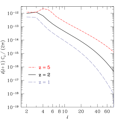
Fig. 4 shows the tensor contribution to $C^{g}_{l}$ for different source redshifts. Here, we have assumed a Gaussian redshift distribution centered on $\tilde{z}$ with RMS width of $0.03(1+\tilde{z})$, emulating the effect of photometric redshift errors. We have kept $b_{e}=2.5,\;Q=1.5$ fixed. While the low multipoles ($l\lesssim 4$) do not depend very strongly on $\tilde{z}$, the contribution for higher $l$ grows by an order of magnitude when going from $\tilde{z}=1$ to $\tilde{z}=2$, and from $\tilde{z}=2$ to $\tilde{z}=5$. We found that reducing the width $\Delta\tilde{z}$ of the redshift distribution has no impact on the results at relevant $l$. The reason is that the bulk of the tensor mode contribution comes from near horizon-scale modes, as tensor modes decay once they enter the horizon. Such long-wavelength modes are not affected by averaging over a reasonably narrow redshift window ($\Delta\tilde{z}<1$).

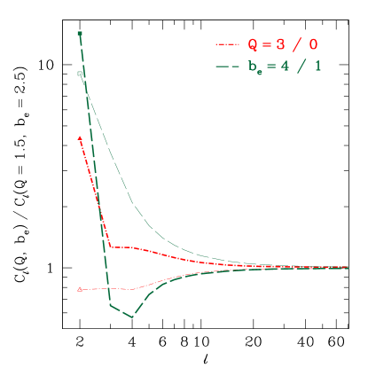
Fig. 5 shows the effect of varying the galaxy sample parameters $b_{e}$, quantifying the redshift evolution of the average number density, and $\mathcal{Q}$, which determines the magnification bias contribution. We see a significant effect at low multipoles when varying $\mathcal{Q}$ and especially $b_{e}$. This is not surprising since we have seen that there is a high degree of cancelation between different terms at low $l$ (Figs. 1 and 2), so that varying the coefficients of the different terms can have a large impact.

On the other hand, $C^{g}_{l}$ is insensitive to changes in $b_{e}$ and $\mathcal{Q}$ for $l\gtrsim 10$. While surprising initially, this fact can be understood straightforwardly. At high $l$, the contributions from $h^{\prime}_{\parallel}$ dominate (Fig. 1). Specifically, following Eq. (39) there are two contributions, $f^{\prime}_{\tilde{\chi}}h^{\prime}_{\parallel}$ and $f^{\prime}\int h^{\prime}_{\parallel}d\chi$. The former contribution is a pure line-of-sight volume distortion effect, and the coefficient $f^{\prime}_{\tilde{\chi}}\propto H^{-1}(\tilde{z})$ is independent of the galaxy sample. Now consider a single Fourier mode contributing to both terms. Neglecting factors of order unity, we can estimate the ratio between the two terms as

$$\frac{f^{\prime}\int_{0}^{\tilde{\chi}}h^{\prime}_{\parallel}d\chi}{f^{\prime}_{\tilde{\chi}}h^{\prime}_{\parallel}}\sim\> H(\tilde{z})\frac{\int_{0}^{\tilde{\chi}}T^{\prime}_{T}(k(\eta_{0}-\chi))d\chi}{T^{\prime}_{T}(k(\eta_{0}-\tilde{\chi}))},$$ (62)

where $T^{\prime}_{T}=dT_{T}/d\eta$. Since $T^{\prime}_{T}$ decays rapidly once the argument $k\eta$ become of order unity, we can approximate the numerator as

$$\int_{0}^{\tilde{\chi}}T^{\prime}_{T}(k(\eta_{0}-\chi))d\chi\sim T^{\prime}_{T}(k(\eta_{0}-\tilde{\chi}))\Delta\chi,$$ (63)

where $\Delta\chi=\Delta(k\eta)/k\sim 1/k$ is the range in $\chi$ that contributes to the integral. Thus, we arrive at an order-of-magnitude estimate of

$$\frac{f^{\prime}\int_{0}^{\tilde{\chi}}h^{\prime}_{\parallel}d\chi}{f^{\prime}_{\tilde{\chi}}h^{\prime}_{\parallel}}\sim\> \frac{H(\tilde{z})}{k}.$$ (64)

Physically, the integral of $h^{\prime}_{\parallel}$ along the line of sight leads to significant cancelations that become more severe as $k$ increases. It is not surprising then that the volume distortion term $f^{\prime}_{\tilde{\chi}}h^{\prime}_{\parallel}$ dominates at high $l$. Specifically, using the kernel $F^{g}_{l}(k)$ for $l=20$ shown in Fig. 2, we can estimate that the typical wavenumber of tensor modes contributing to multipole $l$ is

$$k_{\rm typ}\sim 0.003\>h/{\rm Mpc}\times\frac{l}{10}.$$ (65)

Eq. (64) then says that we expect $f^{\prime}_{\tilde{\chi}}h^{\prime}_{\parallel}$ to dominate for $l\gtrsim 10$, in good agreeement with Fig. 5.

Thus, the line-of-sight volume distortion $\propto h^{\prime}_{\parallel}/H$ is the single dominating term in $C^{g}_{l}$ at high $l$, which explains why the tensor contribution is independent of the galaxy sample at high multipoles. Note however, that the prospects for detecting this effect are mostly restricted to $l\lesssim 10$ anyway due to the steep decline of the signal.

Figure 4: Total tensor mode contribution to the angular galaxy power spectrum as a function of source redshift, for a Gaussian redshift distribution centered on $\tilde{z}$ with an RMS width of $0.03(1+\tilde{z})$. Here, $b_{e}=2.5,\;Q=1.5$ fixed.

Figure 5: Relative impact on the total tensor mode contribution to galaxy clustering when changing $b_{e}$ from 2.5 to 4 and 1 (thick and thin green long-dashed, respectively), and when changing $\mathcal{Q}$ from 1.5 to 3 and 0 (thick and thin red dot-dashed, respectively). Here, a Gaussian redshift distribution centered on $\tilde{z}=2$ with RMS width $0.03(1+\tilde{z})$ was assumed.

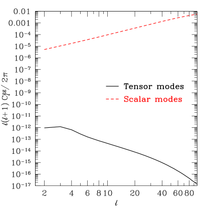
Figure 6: Comparison between tensor mode contributions to the galaxy power spectrum (black solid) for $\tilde{z}=2$ (cf. Fig. 4), and scalar contributions for a linear bias $b=2$ (see App. B for details on the calculation of the scalar contributions).

V Higher order terms

So far, we have only kept terms linear in all perturbations. While all terms second and higher order in $h_{ij}$ are likely irrelevant given the small amplitude of tensor perturbations, there are terms of order $h_{ij}\,\delta_{g}$ which can be much less suppressed on small scales where $\delta_{g}$ can become order unity. There are more terms of order $h_{ij}\,A$ where $A$ stands for any scalar metric perturbation. However, those terms are much smaller than $h_{ij}\,\delta_{g}$ and can be neglected. Note that as long as scalar and tensor modes do not correlate, the lowest non-trivial statistic induced by these terms is a four-point function of $\tilde{\delta}_{g}$. A specific quadratic estimator for the tensor modes can be constructed based on these terms Masui and Pen (2010); Book et al. (2011b). Physically, one uses the anisotropy of the small-scale correlation function of $\tilde{\delta}_{g}$ to search for coherent large-scale distortions induced by tensor modes. Most of the signal-to-noise for detecting a GW background is contained on very small scales Book et al. (2011b).

Noting that $\mathbf{x}=\tilde{\mathbf{x}}-\Delta\mathbf{x}$ and $1+\bar{z}=(1+\tilde{z})(1-\delta z)$, the relevant terms neglected in going from Eq. (30) to Eq. (35) are given by

$$\tilde{\delta}_{gT,\rm 2nd}=\> \delta_{g}\left[\tilde{\mathbf{x}}-\Delta\mathbf{x},(1+\tilde{z})(1-\delta z)-1\right]-\delta_{g}\left(\tilde{\mathbf{x}},\tilde{z}\right)$$

$$=\> -\Delta\mathbf{x}\cdot\mathbf{\nabla}\delta_{g}(\tilde{\mathbf{x}},\tilde{z})-\delta z\frac{\partial}{\partial\ln(1+\tilde{z})}\delta_{g}(\tilde{\mathbf{x}},\tilde{z}),$$ (66)

where $\delta_{g}$ is the intrinsic fractional perturbation in the comoving galaxy density. Note that both $\Delta\mathbf{x}$ and $\delta z$ are linear in $h_{ij}$. If we approximate $\nabla\delta_{g}\sim\delta_{g}/r$, where $r$ is the scale on which the correlation function of $\delta_{g}$ is measured, then the second term is suppressed with respect to the first term by a factor of $r/\tilde{\chi}$, since $\partial\ln\delta_{g}/\partial\ln(1+z)$ is typically order unity. This term is thus highly suppressed on small scales where the second-order terms become relevant. While the intrinsic two-point function $\xi(r)$ of the tracer is isotropic and location-independent (neglecting redshift-space, tidal distortions and intrinsic anisotropy/inhomogeneity Masui and Pen (2010); Jeong and Kamionkowski (2012)), the observed correlation function

$$\tilde{\xi}(\hat{\mathbf{n}},\tilde{z};\hat{\mathbf{n}}^{\prime},\tilde{z}^{\prime})=\langle\tilde{\delta}(\tilde{\mathbf{x}})\tilde{\delta}(\tilde{\mathbf{x}}^{\prime})\rangle$$ (67)

is anisotropic and depends on the location $\tilde{\mathbf{x}}$. This can be used to measure the distortions by tensor perturbations. Specifically, since we have 6 free parameters in $\tilde{\mathbf{x}},\,\tilde{\mathbf{x}}^{\prime}$, we can measure 6 components of the distortion field. At this point, it is important to stress that the terms in Eq. (66) are not observable directly (as a simple example, consider the case of a constant deflection $\Delta\mathbf{x}=$ const). In order to determine which quantities are actually observable, consider contours of constant $\tilde{\xi}$,

$$\tilde{\xi}(\hat{\mathbf{n}},\tilde{z};\hat{\mathbf{n}},\tilde{z}^{\prime})=\xi_{0}.$$ (68)

These contours correpond to a fixed physical scale $r_{0}$ (on a constant-proper-time hypersurface) at the source through

$$\xi(r_{0})=\xi_{0}.$$ (69)

In other words, the intrinsic homogeneous and isotropic correlation function $\xi(r)$ is supplying us with a “standard ruler” $r_{0}$ (or, a set of standard rulers as we are free to vary $\xi_{0}$). In Schmidt and Jeong (2012a), we carefully define a general standard ruler and derive the properties of the deflection field which are observable through it. As we have seen here, the distortion of correlation functions by tensor modes is one application of the results of Schmidt and Jeong (2012a).

Finally, we point out that a non-zero three-leg coupling $\left<\delta(\bm{k}_{1})\delta(\bm{k}_{2})h_{ij}(\bm{k}_{3})\right>$ present at an early stage of the universe can also imprint its signature as a local departure from statistical homogeneity. The optimal estimator for the amplitude of tensor perturbations given such a coupling has been constructed in Jeong and Kamionkowski (2012).

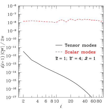
Figure 7: Comparison between tensor mode and scalar contributions to the angular cross-correlation between two widely separated redshift bins ($\tilde{z}=1,\,\tilde{z}^{\prime}=4$) and for $\mathcal{Q}=1$ so that most magnification contributions drop out (linear bias $=2$; other parameters as in Fig. 4).

VI Discussion

We have derived the complete tensor contributions to the observed galaxy density at linear order. The result is summarized in Eq. (39). At this order, gravitational waves do not perturb the intrinsic physical density of tracers; thus all contributions are projection effects from the effects of GW on the propagation of light. We have found that, contrary to gravitational lensing by scalar perturbations, tensor perturbations contribute mainly at redshifts close to the source redshift. Together with the scale-invariant power spectrum of GW, this results in a steeply falling angular power spectrum of the tensor contributions, with multipoles $l\sim 10$ already being suppressed by an order of magnitude with respect to $l=2-4$.

Fig. 6 shows a comparison of the tensor contributions with the scalar contributions to the galaxy density. Here, we have assumed a linear bias of $b=2$, and all relativistic corrections are included following Jeong et al. (2012) (see App. B for details). Clearly, the tensor contributions are suppressed by $\sim$7 orders of magnitude with respect to the scalar contributions at the largest scales, for the maximum currently allowed value of $r=0.2$. One might wonder whether galaxy cross-correlations, i.e. between different redshift bins, could be more promising. After all, when cross-correlating widely separated redshift slices, there is little intrinsic correlation of galaxies, and the main contribution comes from lensing (magnification bias effect $\propto 2(\mathcal{Q}-1)\hat{\kappa}$). Hence, the most optimistic case for detecting tensor modes through their modulation of the galaxy density would consist of cross-correlating two galaxy populations widely separated in redshift, both of which have $\mathcal{Q}=1$ so that the magnification bias effect drops out (this could be achieved, for example, by selecting galaxies on surface brightness). This most optmistic case is shown in Fig. 7. We find that the tensor contribution can become as large as $10^{-3}$ times the residual scalar contribution; however, this is still much too small to be detectable.

Thus, given that we are not able to directly distinguish between scalar and tensor contributions to the galaxy angular power spectrum, we do not expect much detection potential for gravitational waves from the leading order effect on the angular power spectrum of galaxies. However, there are terms of order $h_{ij}\,\delta_{g}$ (where $\delta_{g}$ is the intrinsic galaxy overdensity) which induce a particular four-point correlation function in the observed galaxy density $\tilde{\delta}_{g}$. This is the effect exploited in Masui and Pen (2010); Book et al. (2011b) for projected constraints from 21cm emission from the dark ages. In essence, the intrinsic (homogeneous and isotropic) correlation function provides us with a standard ruler that allows us to observe certain properties of the distortion field, as derived in Schmidt and Jeong (2012a). Thus, one can apply the the scalar-vector-tensor decomposition on the sky described in Schmidt and Jeong (2012a). Most importantly, both the (2-)vector and (2-)tensor components allow for an $E/B$-decomposition, so that any scalar contributions to the distortion (e.g. from lensing or redshift-space distortions) do not contribute to the $B$-mode at linear order. We leave a more detailed investigation of these possibilities for future work.

Appendix A Convergence

We define the convergence through the divergence of the transverse displacements:

$$\hat{\kappa}\equiv\> -\frac{1}{2}\partial_{\perp\,i}\Delta x_{\perp}^{i}$$ (70)

First, taking the transverse divergence of Eq. (27) yields

$$-2\hat{\kappa}=\> \frac{1}{2}\tilde{\chi}\left(h^{i}_{\;j}\partial_{\perp i}\hat{n}^{j}-h_{\parallel}\partial_{\perp i}\hat{n}^{i}\right)_{o}$$ (71)

$$+\int_{0}^{\tilde{\chi}}d\chi\Big{[}\!-\partial_{\perp i}\left(h^{i}_{\;j}\hat{n}^{j}-h_{\parallel}\hat{n}^{i}\right)$$

$$\hskip 42.67912pt+\frac{1}{2}(\tilde{\chi}-\chi)\frac{\chi}{\tilde{\chi}}\nabla_{\perp}^{2}h_{\parallel}\Big{]}.$$

Using the fact that $h_{ij}$ is transverse and that $\partial_{\chi}=\partial_{\parallel}-\partial_{\eta}$, straightforward algebra then yields

$$\hat{\kappa}=\> \frac{5}{4}h_{\parallel o}-\frac{1}{2}h_{\parallel}-\frac{1}{2}\int_{0}^{\tilde{\chi}}d\chi\Big{[}h_{\parallel}^{\prime}+\frac{3}{\chi}h_{\parallel}\Big{]}$$

$$-\frac{1}{4}\nabla^{2}_{\Omega}\int_{0}^{\tilde{\chi}}d\chi\frac{\tilde{\chi}-\chi}{\tilde{\chi}\>\chi}h_{\parallel}.$$ (72)

The last term is familiar as the one dominating on small scales (Newtonian limit) for the scalar case, and is shown separately as blue dotted lines in Fig. 1 and Fig. 3. Note that due to the very different power spectrum of tensor modes, and the fact that tensor modes decay with decreasing redshift, this term actually becomes suppressed on small scales.

Appendix B Angular galaxy power spectrum from scalar perturbations

In this section, we provide expressions for the angular power spectrum of galaxies due to scalar perturbations (see Fig. 6 and 7), including all relativistic corrections as derived in Yoo et al. (2009); Challinor and Lewis (2011); Bonvin and Durrer (2011); Jeong et al. (2012).

It is convenient to use expressions in conformal-Newtonian gauge, where we write the metric as

$$ds^{2}=a^{2}(\eta)\left[-(1+2\Psi)d\eta^{2}+(1+2\Phi)\delta_{ij}dx^{i}dx^{j}\right].$$ (73)

Further, for convenience we write the velocity $v_{i}$ in terms of a scalar velocity potential $V$, $v_{i}=V_{,i}$, and relate $V,\,\Phi,\,\Psi$ to the density contrast $\delta_{m}^{\rm sc}$ in synchronous-comoving gauge through (see Schmidt (2008); Hu and Sawicki (2007))

$$V(\mathbf{k},\eta)=\> aHfk^{-2}D(a(\eta))\delta_{m}^{\rm sc}(\mathbf{k},\eta_{0})$$

$$\Phi(\mathbf{k},\eta)-\Psi(\mathbf{k},\eta)=\> D_{\Phi_{-}}(k,\eta)\delta_{m}^{\rm sc}(\mathbf{k},\eta_{0})$$

$$\Phi(\mathbf{k},\eta)+\Psi(\mathbf{k},\eta)=\> g(k,\eta)D_{\Phi_{-}}(k,\eta)\delta_{m}^{\rm sc}(\mathbf{k},\eta_{0})$$

$$\Rightarrow\Phi(\mathbf{k},\eta)=\> \frac{1}{2}[g+1]D_{\Phi_{-}}\delta_{m}^{\rm sc}(\mathbf{k},\eta_{0})$$

$$\Psi(\mathbf{k},\eta)=\> \frac{1}{2}[g-1]D_{\Phi_{-}}\delta_{m}^{\rm sc}(\mathbf{k},\eta_{0})$$

$$(\Phi-\Psi)^{\prime}(\mathbf{k},\eta)=\> D_{\rm ISW}(k,\eta)\delta_{m}^{\rm sc}(\mathbf{k},\eta_{0}),$$ (74)

where $f\equiv d\ln D/d\ln a$, $D(a)$ is the matter growth factor (normalized to unity at $a=1$) and we have defined general coefficient functions $D_{\Phi_{-}},\,g,\,D_{\rm ISW}$ to allow for non-standard cosmologies. In a $\Lambda$CDM cosmology, we have

$$D_{\Phi_{-}}(\mathbf{k},\eta)=\> 3\Omega_{m}\frac{a^{2}H^{2}}{k^{2}}D(a(\eta))=3\Omega_{m0}\frac{H_{0}^{2}}{k^{2}}a^{-1}(\eta)D(a(\eta))$$

$$g(\mathbf{k},\eta)=\> 0.$$ (75)

Here, the subscript $0$ denotes that the quantity is evaluated at $z=0$. Throughout, we will drop observer terms corresponding to the monopole and dipole, but keep terms that contribute to the quadrupole.

Converting Eqs. (55) and (72) in Jeong et al. (2012) from synchronous-comoving gauge to conformal-Newtonian gauge, using the relations given in App. D of Jeong et al. (2012), we obtain (see also Challinor and Lewis (2011))

$$\tilde{\delta}_{g}(\tilde{\mathbf{x}})=\> \delta_{g}+b_{e}(\delta z-aHV)-\frac{1}{aH}\partial_{\parallel}^{2}V$$

$$-\left(1-\frac{1}{aH}\frac{dH}{dz}+\frac{2}{aH\tilde{\chi}}\right)_{\tilde{z}}[\delta z-aHV]$$

$$+2(\Phi+aHV)$$

$$-\frac{2}{\tilde{\chi}}V-\frac{2}{\tilde{\chi}}\int_{0}^{\tilde{\chi}}d\chi(\Phi-\Psi)-2\kappa$$

$$-\frac{1}{aH}\left(\Phi+aHV\right)^{\prime}+\mathcal{Q}\mathcal{M}$$

$$\mathcal{M}=\> -2\Phi-2aHV+\frac{2}{\tilde{\chi}}V+2\kappa$$

$$+\frac{2}{\tilde{\chi}}\int_{0}^{\tilde{\chi}}(\Phi-\Psi)d\chi+2\left[\frac{1}{aH\tilde{\chi}}-1\right](\delta z-aHV),$$

where

$$\delta z=\> \partial_{\parallel}V-\Psi+\int_{0}^{\tilde{\chi}}d\chi(\Phi-\Psi)^{\prime}$$

$$\kappa=\> -\frac{1}{2}\int_{0}^{\tilde{\chi}}d\chi(\tilde{\chi}-\chi)\frac{\chi}{\tilde{\chi}}\nabla_{\perp}^{2}(\Phi-\Psi)$$ (76)

denote the redshift perturbation and convergence, respectively, in conformal-Newtonian gauge. Assuming a linear bias relation in synchronous-comoving gauge (as discussed in Jeong et al. (2012)), and expanding the different contributions, we obtain

$$\tilde{\delta}_{g}(\tilde{\mathbf{x}})=\> b\delta_{m}^{\rm sc}$$

$$+\left[b_{e}-1-2\mathcal{Q}+\frac{1}{aH}\frac{dH}{dz}+2(\mathcal{Q}-1)\frac{1}{aH\tilde{\chi}}\right]\delta z$$

$$+\left[(3-b_{e})aH-\frac{dH}{dz}\right]V+2(1-\mathcal{Q})\Phi$$

$$+2(\mathcal{Q}-1)\int_{0}^{\tilde{\chi}}\frac{d\chi}{\tilde{\chi}}(\Phi-\Psi)+2(\mathcal{Q}-1)\kappa$$

$$-\frac{1}{aH}\left[\partial_{\parallel}^{2}V+(\Phi+aHV)^{\prime}\right].$$ (77)

We can now evaluate the contribution of a single plane wave along the $z$-axis, i.e. $\delta^{\rm sc}_{m}(\mathbf{x},\eta)=\delta^{\rm sc}_{m}(\mathbf{k},\eta_{0})D(a(\eta))e^{i\mathbf{x}\mathbf{k}}$. Further, we write $\mathbf{x}=\hat{\mathbf{n}}\chi$, and $\mathbf{x}\cdot\mathbf{k}=x\mu$ with $x=k\chi$, $\tilde{x}=k\tilde{\chi}$. First, we have

$$\delta z=\> \delta_{m}^{\rm sc}(\mathbf{k},\eta_{0})\left[\left(\frac{aHfD}{k}\partial_{\tilde{x}}-\frac{1}{2}(g-1)D_{\Phi_{-}}\right)_{\tilde{z}}e^{i\tilde{x}\mu}+\int_{0}^{\tilde{\chi}}d\chi D_{\rm ISW}e^{ix\mu}\right]$$

$$\kappa=\> \frac{1}{2}l(l+1)\int_{0}^{\tilde{\chi}}d\chi\frac{\tilde{\chi}-\chi}{\chi\tilde{\chi}}D_{\Phi_{-}}(k,\eta_{0}-\chi)e^{ix\mu}\>\delta_{m}^{\rm sc}(\mathbf{k},\eta_{0})$$

$$\partial_{\parallel}^{2}V=\> (aHfD)_{\tilde{z}}\,\partial_{\tilde{x}}^{2}e^{i\tilde{x}\mu}\,\delta_{m}^{\rm sc}(\mathbf{k},\eta_{0})$$

$$\Phi^{\prime}=\> \frac{1}{2}\left(g^{\prime}D_{\Phi_{-}}+[g+1]D_{\rm ISW}\right)_{k,\tilde{\eta}}e^{i\tilde{x}\mu}\delta_{m}^{\rm sc}(\mathbf{k},\eta_{0})$$

$$\frac{1}{aH}(aHV)^{\prime}=\> \left(\frac{aH}{k}\right)_{\tilde{z}}^{2}(fD)_{\tilde{z}}\left[2\frac{d\ln aH}{d\ln a}+\frac{d\ln fD}{d\ln a}\right]_{\tilde{z}}e^{i\tilde{x}\mu}\delta_{m}^{\rm sc}(\mathbf{k},\eta_{0}).$$ (78)

Following the procedure described in App. A1 of Schmidt and Jeong (2012a), it is then straightforward to derive the angular power spectrum of $\tilde{\delta}_{g}$, for a sharp source redshift $\tilde{z}$, in terms of the matter power spectrum today $P_{m}(k)$ in synchronous-comoving gauge:

$$C_{\tilde{g}}(l)=\> \frac{2}{\pi}\int k^{2}dk\,P_{m}(k)|F_{l}^{\tilde{g}}(k)|^{2}$$

$$F_{l}^{\tilde{g}}(k)=\> bD(\tilde{a})j_{l}(\tilde{x})+\left[b_{e}-1-2\mathcal{Q}+\frac{1}{aH}\frac{dH}{dz}+2(\mathcal{Q}-1)\frac{1}{aH\tilde{\chi}}\right]_{\tilde{z}}\,F_{l}^{\delta z}(k)$$

$$+\left[(3-b_{e})-\frac{1}{aH}\frac{dH}{dz}\right]_{\tilde{z}}\,\left(\frac{aH}{k}\right)_{\tilde{z}}^{2}(fD)_{\tilde{z}}\,j_{l}(\tilde{x})+2(1-\mathcal{Q})\frac{1}{2}([g+1]D_{\Phi_{-}})_{\tilde{z}}\,j_{l}(\tilde{x})$$

$$+2(\mathcal{Q}-1)\left[\int_{0}^{\tilde{\chi}}\frac{d\chi}{\tilde{\chi}}D_{\Phi_{-}}j_{l}(x)+\frac{1}{2}l(l+1)\int_{0}^{\tilde{\chi}}d\chi\frac{\tilde{\chi}-\chi}{\chi\tilde{\chi}}D_{\Phi_{-}}j_{l}(x)\right]-(fD)_{\tilde{z}}\,\partial_{\tilde{x}}^{2}j_{l}(\tilde{x})$$

$$-\frac{1}{aH}\frac{1}{2}\left(g^{\prime}D_{\Phi_{-}}+[g+1]D_{\rm ISW}\right)_{\tilde{z}}\,j_{l}(\tilde{x})-\left(\frac{aH}{k}\right)_{\tilde{z}}^{2}(fD)_{\tilde{z}}\,\left[2\frac{d\ln aH}{d\ln a}+\frac{d\ln fD}{d\ln a}\right]_{\tilde{z}}\,j_{l}(\tilde{x})$$ (79)

$$F_{l}^{\delta z}(k)=\> \left(\frac{aHfD}{k}\partial_{\tilde{x}}-\frac{1}{2}(g-1)D_{\Phi_{-}}\right)_{\tilde{z}}j_{l}(\tilde{x})+\int_{0}^{\tilde{\chi}}d\chi D_{\rm ISW}j_{l}(x),$$ (80)

where again $x=k\chi,\,\tilde{x}=k\tilde{\chi}$. We can also easily derive the power spectrum of the magnification itself, which is an observable (see Schmidt and Jeong (2012a)):

$$C_{\mathcal{M}}(l)=\> \frac{2}{\pi}\int k^{2}dk\,P_{m}(k)|F_{l}^{\mathcal{M}}(k)|^{2}$$

$$F_{l}^{\mathcal{M}}(k)=\> 2\left[\frac{1}{aH\tilde{\chi}}-1\right]F_{l}^{\delta z}(k)-([g+1]D_{\Phi_{-}})_{\tilde{z}}\,j_{l}(\tilde{x})$$

$$+l(l+1)\int_{0}^{\tilde{\chi}}d\chi\frac{\tilde{\chi}-\chi}{\chi\tilde{\chi}}D_{\Phi_{-}}j_{l}(x)+2\int_{0}^{\tilde{\chi}}\frac{d\chi}{\tilde{\chi}}D_{\Phi_{-}}j_{l}(x).$$ (81)

These expressions are for a sharp source redshift. It is straightforward to generalize them to a distribution $dN/d\tilde{z}$ of source redshifts (where $dN/d\tilde{z}$ is assumed normalized), following the discussion in § IV.1. In particular, contributions to $F^{X}_{l}(k)$ of the form

$$\int_{0}^{\tilde{\chi}}d\chi\,W(\tilde{\chi},\chi)\hat{Q}(x)j_{l}(x),$$ (82)

where $\hat{Q}(x)$ is any derivative operator, are generalized to

$$\int_{0}^{\tilde{\chi}}d\chi\,W(\tilde{\chi},\chi)\hat{Q}(x)j_{l}(x)\to\> \int_{0}^{\infty}d\chi\,\mathcal{W}(\chi)\hat{Q}(x)j_{l}(x)$$

$$\mathcal{W}(\chi)=\> \int_{z(\chi)}^{\infty}d\tilde{z}\,\frac{dN}{d\tilde{z}}W(\tilde{\chi}=\bar{\chi}(\tilde{z}),\chi).$$ (83)

Further, contributions evaluated at the source are generalized to

$$A(\tilde{\chi})\hat{Q}(\tilde{x})j_{l}(\tilde{x})\to\> \int_{0}^{\infty}d\chi\,\mathcal{W}(\chi)\hat{Q}(x)j_{l}(x)$$

$$\mathcal{W}(\chi)=\> \left[\frac{dN}{dz}H(z)\right]_{z(\chi)}\!\!A(\chi).$$ (84)

References

• Schmidt and Jeong (2012a) F. Schmidt and D. Jeong (2012a), eprint 1204.3625.
• Starobinsky (1980) A. A. Starobinsky, Phys. Lett. B 91, 99 (1980).
• Guth (1981) A. H. Guth, Phys. Rev. D 23, 347 (1981).
• Seljak and Zaldarriaga (1997) U. Seljak and M. Zaldarriaga, Physical Review Letters 78, 2054 (1997), eprint arXiv:astro-ph/9609169.
• Kamionkowski et al. (1997) M. Kamionkowski, A. Kosowsky, and A. Stebbins, Phys. Rev. Lett. 78, 2058 (1997), URL http://link.aps.org/doi/10.1103/PhysRevLett.78.2058.
• Linder (1988) E. V. Linder, Astrophys. J.  328, 77 (1988).
• Bar-Kana (1996) R. Bar-Kana, Phys. Rev. D 54, 7138 (1996), eprint arXiv:astro-ph/9606065.
• Book and Flanagan (2011) L. G. Book and É. É. Flanagan, Phys. Rev. D 83, 024024 (2011), eprint 1009.4192.
• Bharadwaj and Guha Sarkar (2009) S. Bharadwaj and T. Guha Sarkar, Phys. Rev. D 79, 124003 (2009), eprint 0901.3655.
• Book et al. (2011a) L. G. Book, M. Kamionkowski, and T. Souradeep, ArXiv e-prints (2011a), eprint 1109.2910.
• Masui and Pen (2010) K. W. Masui and U.-L. Pen, Physical Review Letters 105, 161302 (2010), eprint 1006.4181.
• Book et al. (2011b) L. Book, M. Kamionkowski, and F. Schmidt, ArXiv e-prints (2011b), eprint 1112.0567.
• Dodelson et al. (2003) S. Dodelson, E. Rozo, and A. Stebbins, Physical Review Letters 91, 021301 (2003), eprint arXiv:astro-ph/0301177.
• Dodelson (2010) S. Dodelson, Phys. Rev. D 82, 023522 (2010), eprint 1001.5012.
• Schmidt and Jeong (2012b) F. Schmidt and D. Jeong (2012b), eprint 1205.1514.
• Yoo et al. (2009) J. Yoo, A. L. Fitzpatrick, and M. Zaldarriaga, Phys. Rev. D 80, 083514 (2009), eprint 0907.0707.
• Challinor and Lewis (2011) A. Challinor and A. Lewis, ArXiv e-prints (2011), eprint 1105.5292.
• Bonvin and Durrer (2011) C. Bonvin and R. Durrer, ArXiv e-prints (2011), eprint 1105.5280.
• Jeong et al. (2012) D. Jeong, F. Schmidt, and C. M. Hirata, Phys. Rev. D 85, 023504 (2012), eprint 1107.5427.
• Kaiser and Jaffe (1997) N. Kaiser and A. Jaffe, Astrophys. J.  484, 545 (1997), eprint arXiv:astro-ph/9609043.
• Komatsu et al. (2011) E. Komatsu, K. M. Smith, J. Dunkley, C. L. Bennett, B. Gold, G. Hinshaw, N. Jarosik, D. Larson, M. R. Nolta, L. Page, et al., Astrophys. J. Supp. 192, 18 (2011), eprint 1001.4538.
• Schmidt et al. (2009) F. Schmidt, E. Rozo, S. Dodelson, L. Hui, and E. Sheldon, Physical Review Letters 103, 051301 (2009), eprint 0904.4702.
• Limber (1954) D. Limber, Astrophys. J. 119, 655 (1954).
• (24) URL http://www.lsst.org.
• Jeong and Kamionkowski (2012) D. Jeong and M. Kamionkowski, ArXiv e-prints (2012), eprint 1203.0302.
• Schmidt (2008) F. Schmidt, Phys. Rev. D 78, 043002 (2008), eprint 0805.4812.
• Hu and Sawicki (2007) W. Hu and I. Sawicki, Phys. Rev. D 76, 104043 (2007), eprint 0708.1190.