Type Ia Supernovae Selection
and
Forecast of Cosmology Constraints
for the Dark Energy Survey
Abstract
We present the results of a study of selection criteria to identify Type Ia supernovae photometrically in a simulated mixed sample of Type Ia supernovae and core collapse supernovae. The simulated sample is a mockup of the expected results of the Dark Energy Survey. Fits to the MLCS2k2 and SALT2 Type Ia supernova models are compared and used to help separate the Type Ia supernovae from the core collapse sample. The Dark Energy Task Force Figure of Merit (modified to include core collapse supernovae systematics) is used to discriminate among the various selection criteria. This study of varying selection cuts for Type Ia supernova candidates is the first to evaluate core collapse contamination using the Figure of Merit. Different factors that contribute to the Figure of Merit are detailed. With our analysis methods, both SALT2 and MLCS2k2 Figures of Merit improve with tighter selection cuts and higher purities, peaking at 98% purity.
1 Motivation
In the next decade, the number of detected Type Ia supernovae (SNIa) will increase dramatically [1, 2], surpassing the resources available for spectroscopic confirmation of each supernova (SN). This has produced an increased interest in the photometric identification of SNIa in samples including significant numbers of core collapse supernovae (SNcc). In order to improve the contraints on the accelerated expansion of the universe, discovered with SNIa in the late 1990’s [3, 4], photometric typing of supernovae (SNe) must be very robust. Two recent studies of simulated SNe have approached the subject of SN photometric identification in different ways: 1) the first, Kessler et al. (2010) [5], compared a wide variety of photometric-typing algorithms, but did not evaluate the impact on cosmology constraints, 2) the second, Bernstein et al. (2011) [1] studied the impact on cosmology in detail, but only used one photometric-typing algorithm (MLCS2k2 fit quality cuts). The analysis presented in this paper is a follow-up to Bernstein et al., and incorporates several new features in the analysis.
Using tight signal-to-noise ratio (SNR) cuts and a SNIa fit quality cut (MLCS2k2 model [6]), Ref. [1] achieved a purity (SNIa/Total) above 95%. The remaining SNcc had a negligible effect on cosmology. This was achieved for the case where the redshifts of the SNe were assumed to be measured accurately in a spectroscopic follow-up of the host galaxies. In this article, we follow a similar approach but extend the analysis by studying the effects of relaxing the SNR cuts and including the SALT2 SNIa model fit quality. We use data samples simulated for the 10-field hybrid footprint of the Dark Energy Survey111http://www.darkenergysurvey.org (DES), performed with the SNANA package as in Ref. [1]. We have updated the SNcc simulation inputs to reflect improved knowledge of their relative fractions and brightnesses (see section 2). We present four distinct sets of SNR cuts for both the MLCS2k2 and SALT2 models (using the SALT2mu procedure in Ref. [7] to obtain distance moduli for the SALT2 model).222The SALT2 simulations used and . The SALT2mu evaluation of the distance modulus also used the same fixed values of and . The fitting of and , in the presence of significant SNcc contamination, is beyond the scope of this paper. The quantity SNRMAX is defined to be the SNR at the measured epoch of maximum signal-to-noise in each of the four DES broadband filters used in the supernova analysis. Within a single survey strategy in terms of average observing conditions and cadence, this quantity may be used as a rough proxy for how well the supernova light curve was measured. Our goal is to find the purity levels that optimize the Dark Energy Task Force (DETF) [8] Figure of Merit (FoM). One obvious question is: What is a significant level of change in FoM? Our goal is to have the uncertainty in FoM due to the SNcc sample to be much smaller than the largest uncertainty in Ref. [1], which was due to the filter zeropoint uncertainty. The filter zeropoint uncertainty caused a 70 unit reduction in the FoM (30%). Therefore, we consider changes of 10% to be significant in our analysis. We are not considering the entire suite of systematic uncertainties in this analysis, only the impact of photometric typing and selection cuts for the mixed SNe sample.
The outline of the paper is as follows. We present the changes in the simulation of the SNcc sample in 2. Our variety of SNR selection criteria, the SNIa models we are using, and the resulting purities and efficiencies are presented in 3. The DETF Figure of Merit calculation, some relevant factors and examples, and the final results are presented in 4. We discuss the results in 5 and include more details of the new simulation inputs in Appendix A. Finally, we include supplementary figures in Appendix B.
2 Supernova Sample Simulations
The SNANA package [9] is used to simulate the light curves of the 5-year SNIa and SNcc samples for the DES. The simulations are very similar to those in Ref. [1] but have been updated and improved with more recent information. The list of changes since Ref. [1] are:
-
•
The SNANA version was updated to v9_89b from v8_37. Our model choices were MLCS2k2.v007 and SALT2.LAMOPEN.
- •
- •
- •
-
•
We now use separate relative fractions for SN Types Ib and Ic, as well as different average brightnesses based on Li et al.. (Type II SNe already had separate relative fractions in [1].)
-
•
Since the Li et al. sample is complete, and the absolute brightnesses are not corrected for dust extinction, our simulation does not include dust extinction applied to the SNcc sample.
-
•
The widths of the absolute brightness distributions for each type of SNcc template are matched to the measured widths from Li et al.
The details of these changes are available in Appendix A. The changes mostly cancel each other in terms of the overall purity of the sample with Ref. [1] cuts. The relative mixture of the SNcc sample passing cuts is more uniform, however, with less dominance from the Type Ibc SNe.
3 Selection Criteria and Type Ia SN models
3.1 Supernova Sample Signal-to-Noise Cuts
As mentioned previously, our SNR is defined at the measured epoch of maximum SNR in each filter (SNRMAX). We present four distinct sets of SNR cuts for both the MLCS2k2 and SALT2 models. For simplicity, we define the symbols used in the rest of the paper for these four sets of cuts in Tab. 1.
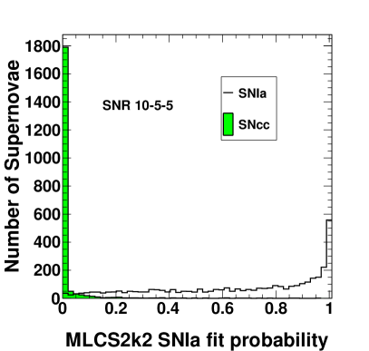
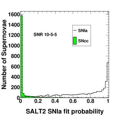
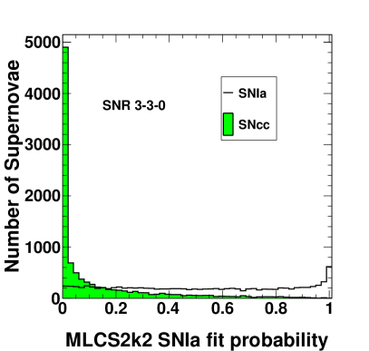
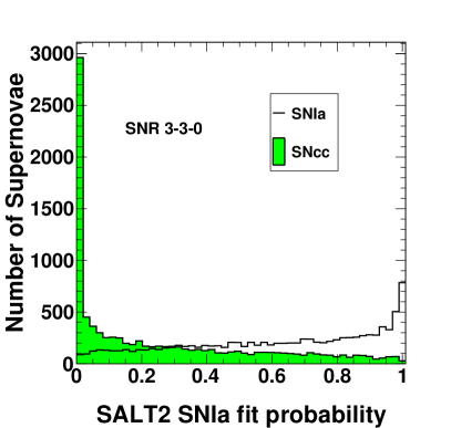
| Cuts | Symbol |
|---|---|
| 2 filters with SNRMAX | SNR-3-3-0 |
| 2 filters with SNRMAX | SNR-5-5-0 |
| 3 filters with SNRMAX | SNR-5-5-5 |
| 1 filter SNRMAX , 2 more filters SNRMAX | SNR-10-5-5 |
3.2 Type Ia Model Fit Probabilities
Core collapse SNe light curves fit to a SNIa light curve model might be expected to have bad fit qualities, and this was demonstrated in Ref. [1]. Motivated by this, we reject SN candidates which have deviations from the best fit light curve model (whether MLCS2k2 or SALT2) that are statistically large compared to the errors. This is quantified in terms of fit probabilities333If the observed deviations from the best fit model were due to Gaussian fluctuations compatible with the reported errors on observations, this is the probability of the being larger than the observed for the number of degrees of freedom in the light curve fit. obtained from the light-curve and the number of degrees of freedom. Figure 1 shows the results of the fit probabilities for both models, and for our tightest and loosest cuts. It is evident that the SALT2 model has larger fit probabilities for the SNcc sample and hence we obtain lower purities for SALT2 compared to those of MLCS2k2. This is most likely due to the use of tight dust extinction priors used in the MLCS2k2 fits [1]. But as described in Ref. [1], these MLCS2k2 priors lead to additional SNe color systematics not present in SALT2 fits.
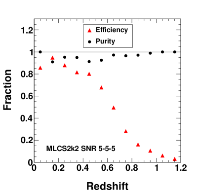
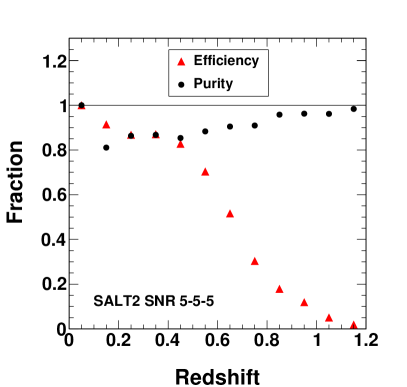
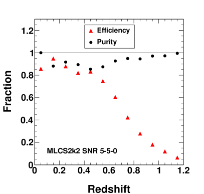
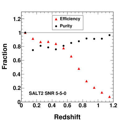
3.3 Purities and Efficiencies
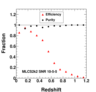
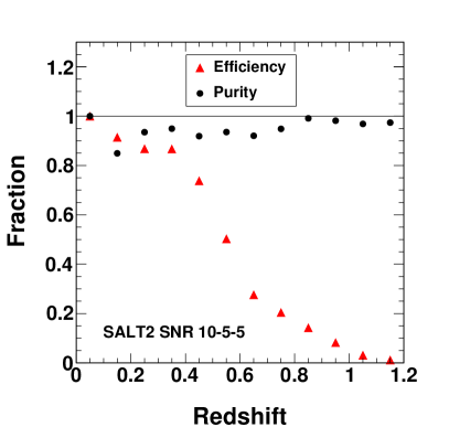
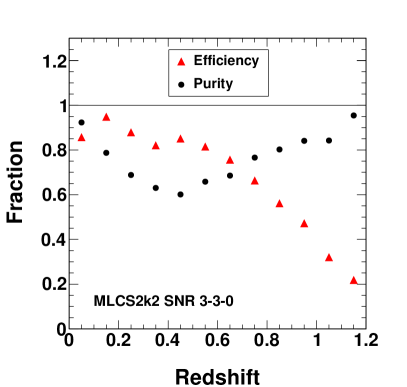
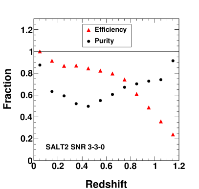
In this section, we present the results for purities and SNIa efficiencies for the four sets of SNRMAX cuts and with the MLCS2k2 and SALT2 fit probability cuts described above. We define the SNIa efficiency as the ratio of the number of SNIa passing all cuts that define the sample to the total number of SNIa simulated. For our calculation of efficiency, the denominator is the complete sample of SNIa generated with zero SNR cuts and the rates described in Ref. [1]. Many studies of SNIa efficiencies apply different sets of base SNR cuts, making it difficult to compare efficiencies from different analyses. We define the sample purity as the ratio of the number of SNIa to the total number of SNIa+SNcc passing all cuts. The numbers of SNIa and SNcc and the related purities and efficiencies integrated over all redshifts are presented in Tab. 2. Figure 2 shows the purities and efficiencies as functions of redshift for the tightest and loosest SNR cuts for both the MLCS2k2 and SALT2 models. As discussed above for Fig. 1, the SALT2 model without tight priors is more flexible and leads to lower purities than our current implementation of the MLCS2k2 model.
| SNRMAX Cuts | Algorithm | SNIa | SNcc | Purity | Efficiency |
|---|---|---|---|---|---|
| SNR-10-5-5 | MLCS | 3534 | 88 | 98% | 20% |
| SNR-5-5-5 | MLCS | 4659 | 240 | 95% | 27% |
| SNR-5-5-0 | MLCS | 5949 | 534 | 92% | 34% |
| SNR-3-3-0 | MLCS | 9206 | 3138 | 75% | 53% |
| SNR-10-5-5 | SALT | 3686 | 236 | 94% | 21% |
| SNR-5-5-5 | SALT | 4820 | 568 | 89% | 27% |
| SNR-5-5-0 | SALT | 6425 | 1173 | 85% | 37% |
| SNR-3-3-0 | SALT | 9776 | 5298 | 65% | 56% |
| Type | Bernstein et al. | This Analysis |
|---|---|---|
| Ib/c | 57 | 54 |
| IIP | 2 | 5 |
| IIn | 2 | 0 |
| IIL | 2 | 29 |
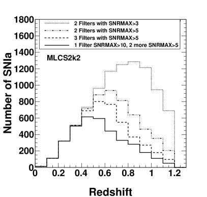
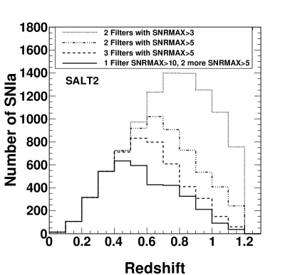
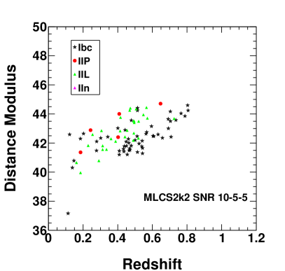
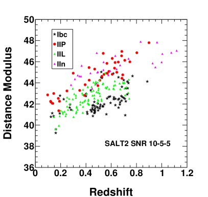
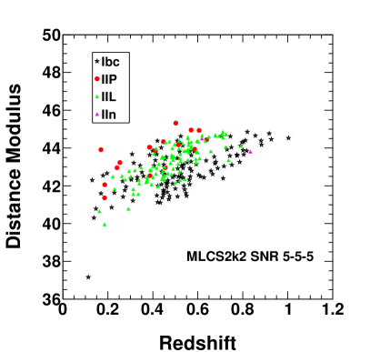
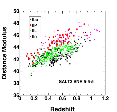
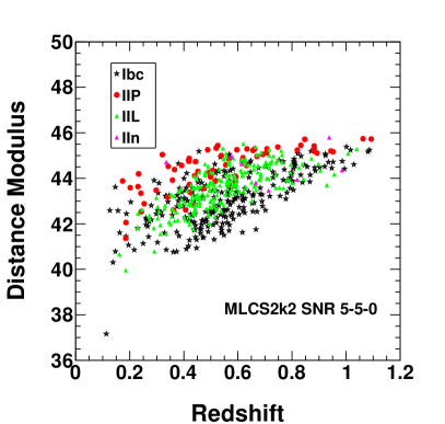
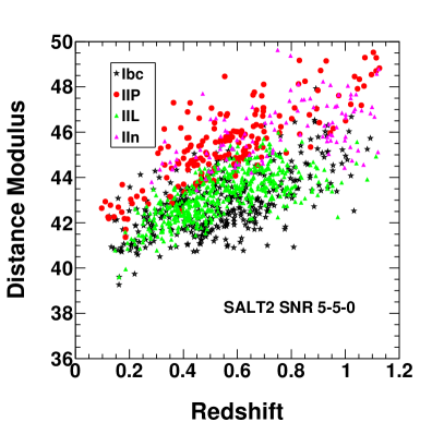
Figure 3 shows some characteristics of the SNIa and SNcc samples that pass the fit probability cuts. The SNIa redshift distributions shown on the top panel demonstrate the increasing SNIa efficiency at large redshift as the cuts are relaxed. The top left panel is for MLCS2k2 and the top right panel is for the SALT2 model. The Hubble scatter shown on the lower panels is for the SNcc sample passing the SNR-10-5-5 cuts and a fit probability cut in each case. The number of type IIL SNcc is significantly more than in Ref. [1]. The numbers for each SNcc type with the SNR-10-5-5 cuts are shown in Tab. 3. This change in SNcc numbers is due to the simulation input changes described in 2 and Appendix A.
4 Dark Energy Task Force Figure of Merit
4.1 Figure of Merit Calculation
As described in Ref. [1], constraints on cosmological parameters are obtained by comparing the predicted theoretical values of distance moduli, , to the values inferred from the light curve fits of the SN simulations, , where: is the set of cosmological parameters. Here, and are the current energy densities corresponding to Dark Energy and spatial curvature as a fraction of the critical density. The parameters are the parameters in a CPL parametrization [13, 14] of the equation of state: The likelihood for an individual SN, at redshift zi, is taken to be a Gaussian with a mean given by the at redshift zi for the cosmological parameters . The simulated SN observations are independent and the likelihood is analytically marginalized over the nuisance-parameter combination of the Hubble Constant, , and the absolute magnitude, , with a flat prior on . Following the DETF Report [8], we evaluated the performance of photometric identication algorithms and selection criteria in terms of the DETF FoM.
The distance modulus errors used in the FoM calculation are typically derived from the light curve fit errors and an intrinsic dispersion added in quadrature as in Ref. [1]. For a pure SNIa sample, the intrinsic dispersion is chosen to give (DOF=number of degrees of freedom) in the cosmology fit. This procedure works for a very pure sample but will fail to account for the additional dispersion due to SNcc contamination. Therefore, we will take an additional step in this analysis of determining the RMS of the total SNIa+SNcc sample in each of 12 redshift bins. We then inflate the input errors for the FoM calculation by adding an additional amount in quadrature to the reported errors such that the means of the inflated errors match those RMS values. This ensures a reasonable in the cosmology fit. Whenever we use inflated errors in the FoM calculation we do not include the 0.13 intrinsic dispersion.
We model the issue of core collapse contamination in the Figure of Merit calculation in a way similar to the method used in Ref. [1]. We assume that the distance modulus obtained by fitting a core collapse supernova to a Ia model is given by
where is the distance modulus and encodes the differences in characteristics of core-collapse supernovae from SNIa and is independent of the cosmology. We expect to be different for each core-collapse supernova (certainly core collapse supernova types and templates), and hence there will be a large scatter in this quantity. For a DES simulation with a fixed set of selection cuts, we expect that , the average value of in each bin, to be roughly consistent between different realizations of simulations. We use our simulated data to determine for each set of selection cuts used in this analysis.
With this information from simulations, we obtain an average correction as a function of redshift for the average shift in introduced by the core-collapse contamination. We parametrize this correction by noting that for a mixed sample the average value of is given by
| (4.1) | |||||
where is the probability that a randomly selected supernova at redshift in the mixed sample is a core collapse supernova, purity, and we have assumed that the observed distance moduli of SNIa are unbiased estimates of the distance moduli . The average correction is the second term in Eqn. 4.1 and the part in the square brackets is computed from simulations and is held fixed. Thus, we expand our set of model parameters to include and study joint constraints on all the parameters including . In order to obtain a Figure of Merit analogous to the DETF FoM, we evaluate a Fisher Matrix at the DETF fiducial values of the cosmological parameters and marginalize over all parameters other than and . In doing so, we use priors on the model parameters. A Gaussian prior on with a standard deviation assumed to be equal to is used. The choices of priors on cosmological parameters are the same as those used in Ref. [1]: a Fisher matrix representing priors on the set of cosmological parameters from DETF StageII experiments and expected Planck data was used along with a set of low redshift supernovae from experiments that were not included in calculating the StageII Fisher matrix mentioned above. These low redshift SNe were spectroscopically identified, and thus neither of the modifications for core-collapse supernovae (the inflation of the reported errors to match RMS or the use of the polynomial) were applied to these supernovae.
4.2 Factors affecting the Figure of Merit
In this section, we investigate various factors that affect the DETF Figure of Merit, and give a step-by-step example of how the FoM changes with each factor. We first investigate our sensitivity to the fit probability cut shown in Fig. 1. We show in Tab. 4 how the FoM changes for fit probabilities greater than 0.05, 0.1 and 0.2, for the tightest (SNR-10-5-5) and loosest (SNR-3-3-0) cuts. The FoM is relatively insensitive to the precise fit probability cut for both MLCS2k2 and SALT2. Therefore for the rest of this paper, we will use 0.1 as the cut point, the same as in Ref. [1].
| SNRMAX cuts | ID algorithm | FoM SNIaSNcc+Sys. |
|---|---|---|
| SNR-10-5-5 | MLCS | 189 |
| SNR-10-5-5 | MLCS | 196 |
| SNR-10-5-5 | MLCS | 198 |
| SNR-3-3-0 | MLCS | 159 |
| SNR-3-3-0 | MLCS | 158 |
| SNR-3-3-0 | MLCS | 155 |
| SNR-10-5-5 | SALT | 132 |
| SNR-10-5-5 | SALT | 132 |
| SNR-10-5-5 | SALT | 140 |
| SNR-3-3-0 | SALT | 105 |
| SNR-3-3-0 | SALT | 104 |
| SNR-3-3-0 | SALT | 103 |
We now investigate four factors that significantly affect the DETF Figure of Merit:
-
•
the number of SNIa (),
-
•
the reported errors on the distance modulus,
-
•
the effect of the additional Hubble scatter due to SNcc, which is usually much larger than the reported errors on the distance modulus,
-
•
the uncertainty in the Hubble residual due to SNcc systematics.
The number of SNe in the sample is an obvious factor to consider. First, let us consider the simple DETF FoM without any of our modifications. Here, adding supernovae to a sample will always improve the FoM. If the supernovae added have the same statistical properties (similar error bars) then the rate of improvement with numbers depends on the priors used in the calculation. This dependence can be observed in the left panel of Fig. 4, where independent statistically equivalent samples of SNIa passing selection cuts SNR-10-5-5 (such as would be obtained by using more seasons of DES observation using the same selection cuts) have been added. The lower curve, approximately linear444The linear dependence on can be understood from the fact that the DETF FoM is inversely proportional to the product of errors on and , each of which fall like ., is the variation of the FoM with no DETF Stage II or Planck priors, and it has been multiplied by 1000 in order to be visible. That demonstrates how critically important the priors are in the FoM. The upper curve includes the DETF stage II and Planck priors and has a dependence555This dependence is difficult to predict due to the complicated effects of the priors..
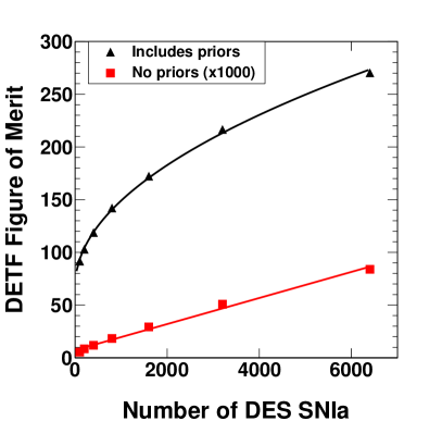
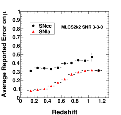
We begin our step-by-step example of FoM changes with the top row of Tab. 5, for the loosest cuts SNR-3-3-0 and MLCS . While 9206 SNIa pass these cuts, these SNIa are not statistically equivalent to the SNIa used in the left panel of Fig. 4, as supernovae that fail the tightest cuts have larger errors on the distance modulus. The FoM value (with priors) of 310 is for the 9206 SNIa that pass these cuts with the reported distance moduli errors added in quadrature with 0.13, as discussed above, and used in Ref. [1]. The value extrapolated from the left panel of Fig. 4 is 316. The difference is even starker for second row of the table, where the FoM=354 is the extrapolated value from the left panel when the number of SN is raised to 12344, the total number of supernovae (SNIa and SNcc) in the sample. The third row of the table shows the calculated FoM of 316 using 0.13 added in quadrature to the reported distance moduli errors. Most of the difference between 354 and 316 is due to the reported errors on the distance moduli of SNcc being larger than SNIa, as shown in the right panel of Fig. 4.
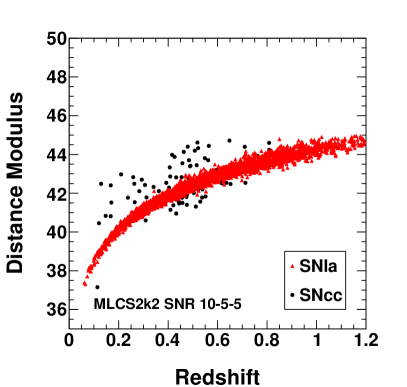
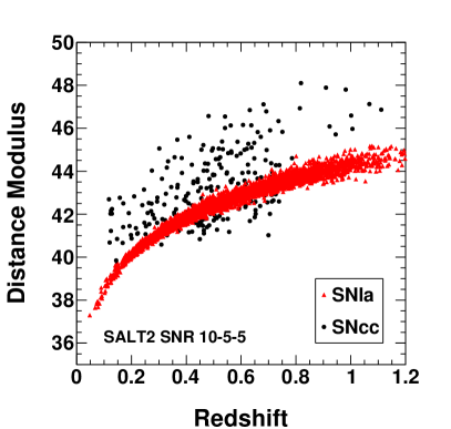
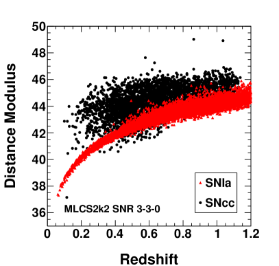
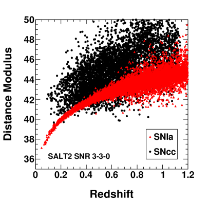
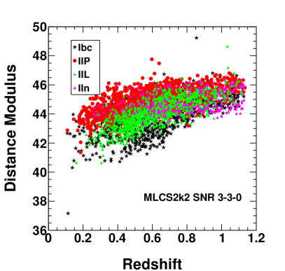
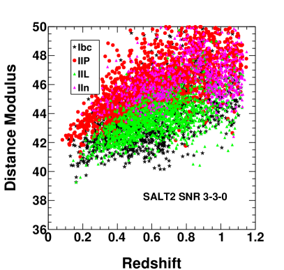
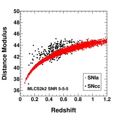
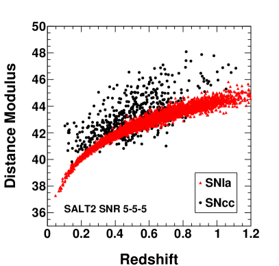
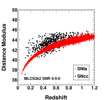
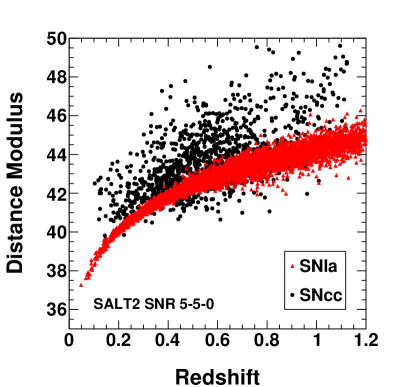
The third factor affecting the FoM is the effect of the SNcc scatter on the Hubble diagram, demonstrated in Fig. 5 for the loosest and tightest SNR cuts for both MLCS2k2 and SALT2 models. As discussed earlier, we inflate the SNIa and SNcc input errors to the FoM determination in order to achieve a reasonable . The additional error added, for the loosest SNR-3-3-0 cuts, varies from 0.8-1.5 mags for SALT2 and 0.3-1.3 mags for the MLCS2k2 model. Our choice of the loosest SNR cuts and MLCS2k2 for our example shows the most dramatic effect of these additional errors in the fourth row of Tab. 5. This shows the FoM decreasing from 316 to 181. Note that this is just an exercise to understand the FoM better. We do not expect anyone to attempt to do a cosmology analysis with the SNcc contamination shown in Fig. 5 with the loosest cuts.
The fourth and final SNcc-related factor we consider that affects the FoM significantly is the strength of SNcc contamination. As discussed above and in Ref. [1], we model as a function of , the change of the Hubble residual due to varying amounts of SNcc contamination, and take 100% of this change as the one standard deviation uncertainty. Figure 6 shows the change in Hubble residual due to the SNcc sample for the loosest cuts and for the MLCS2k2 and SALT2 models. The bottom row of Tab. 5 shows the FoM decreasing from 181 to 158 using the change in Hubble residual with MLCS2k2 and the loosest cuts.
| FoM for Ia only | 310 |
|---|---|
| FoM for SNIa + SNcc (Extrapolating using dependence) | 354 |
| FoM for SNIa + SNcc(using fitter reported SNe error + 0.13 intrinsic dispersion) | 316 |
| FoM for SNIa + SNcc(inflated error for ) | 181 |
| FoM for SNIa + SNcc(inflated error for and SNcc systematic) | 158 |
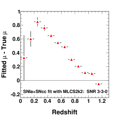
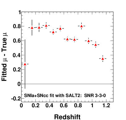
Table 6 shows a summary of our results, combining the four factors that affect the FoM discussed above. We present different values for the FoM, from tighter cuts (SNR-10-5-5) to looser cuts (SNR-3-3-0), for both MLCS2k2 and SALT2 models. The column labeled FoM Ia is for SNIa and incorporates the reported SNIa errors added to 0.13 in quadrature. The column labeled FoM Ia+CC adds the SNcc sample and includes the inflated error to make for each sample. The final column adds the SNcc systematic described above and is the most relevant column. The FoM is best for the tightest cuts for both SALT2 and MLCS2k2 models. SNR cuts tighter than SNR-10-5-5 were also analyzed. It is expected that as the SNR cuts are tightened, and purities approach 100%, the loss in SNIa statistics will cause a drop in FoM. We observe this for both MLCS2k2 and SALT2, but at different SNR cut values in each case. However, for both MLCS2k2 and SALT2, the peak FoM value occured at 98% purity (SNR-10-10-5 and SNR-10-5-5 had almost identical purity and FoM for MLCS2k2 and SNR-10-10-10 had the peak FoM for SALT2).
We observe again that the SALT2 fitter allows more SNcc into our sample than MLCS2k2 and results in lower purities for a given set of SNR cuts. In addition, the Hubble scatter for the SNcc is larger for SALT2 than MLCS2k2. The lower purity and larger scatter cause lower FoM for the samples fit with the SALT2 model. As mentioned earlier, this is at least partly due to the tight dust extinction priors used in the MLCS2k2 fits [1].
| SNRMAX cuts | SNIa ID | SNIa | Pur. | FoM Ia | FoM IaCC | FoM IaCC+Sys. |
|---|---|---|---|---|---|---|
| SNR-10-5-5 | MLCS | 3534 | 98% | 249 | 203 | 196 |
| SNR-5-5-5 | MLCS | 4659 | 95% | 266 | 200 | 172 |
| SNR-5-5-0 | MLCS | 5949 | 92% | 285 | 197 | 167 |
| SNR-3-3-0 | MLCS | 9206 | 75% | 310 | 181 | 158 |
| SNR-10-5-5 | SALT | 3686 | 94% | 234 | 147 | 132 |
| SNR-5-5-5 | SALT | 4820 | 89% | 246 | 151 | 131 |
| SNR-5-5-0 | SALT | 6425 | 85% | 263 | 144 | 120 |
| SNR-3-3-0 | SALT | 9776 | 65% | 276 | 130 | 104 |
5 Discussion
This analysis is an extension of the Bernstein et al. [1] paper with a focus on the Type Ia/core collapse separation. The previous analysis used one set of SNR cuts and one SNIa identification model and found a negligible effect on cosmology. On the other hand, the tight cuts led to a low efficiency for SNIa. It is natural to investigate additional SNR cuts and models.
The main extensions to Ref. [1] addressed in this analysis are listed below:
-
•
four sets of SNR cuts are used instead of one,
-
•
the MLCS2k2 and SALT2 models are treated on equal footing,
-
•
the SNANA simulation inputs for core collapse simulations have been updated with more current knowledge (a total of seven input changes were made and are detailed in Appendix A),
-
•
a variety of fit probability and purity/efficiency plots are presented,
-
•
a detailed purity and efficiency table for all variations is presented,
-
•
the Dark Energy Task Force Figure of Merit is tested on all variations,
-
•
the normal procedure of adding an intrinsic dispersion 0.13 in quadrature with the reported error is supplemented by a new procedure that uses inflated errors determined from the Hubble diagram RMS of the total SNIa+SNcc sample in redshift bins,
-
•
other significant factors in the FoM are examined, such as the scaling with number of supernovae and large impact of the DETF stage II and Planck priors (more than x1000 increase in FoM), as well as the core collapse systematic uncertainty.
The changes to the simulation inputs caused very little change in resulting purities, compared to Ref. [1]. The most significant change is in the Type IIL simulation, which increased in number passing cuts by almost a factor of 15. This is mostly due to the 0.5 magnitude brighter input value to the SNANA template, coming from Ref. [10]. This highlights a fragility in the current knowledge of core collapse simulations, there is only one Type IIL template available to generate the simulations. Hopefully this can be supplemented by more templates in the future.
We find the SALT2 model allows more SNcc passing the fit probability cuts compared to the MLCS2k2 model (which includes dust extinction priors) and leads to somewhat lower purities and lower FoM. The scatter in the SNcc values is also larger for the SALT2 model, and this also contributes to lower FoM with our treatment of core collapse uncertainties. The more significant result, however, is that for both models the FoM decreases with purities lower than 98%. Purities higher than 98% were analyzed and the FoM decreased for both models due to a loss of SNIa statistics.
This analysis lays the groundwork for future analyses of more sophisticated photometric typers [5], as well as the application of additional cuts, such as SNe color and stretch. From the top panels in Fig. 3, it is clear that the SNIa sample is complete up to even with the tightest SNR cuts. Therefore, loosening SNR cuts for low redshift only increases the SNcc contamination. Furthermore, at the purity is increasing even with the loosest cuts. These trends imply that using a -dependent SNR cut would be a better choice.
In addition, it is obvious from the Hubble scatter plots that many of the SNcc are easily removed, as their values are many standard deviations away from any possible cosmology. Coupled with potential cuts, it is necessary to study fitted cosmology biases for each possible sample, since the DETF FoM is not sensitive to these biases. Another challenging future study is the measurement of SNe colors (either SALT2 or MLCS2k2 ), as a function of redshift, in the presence of varying amounts of SNcc contamination. Finally, the treatment of the core collapse systematic (100% of the shift in Hubble residual) is simplistic and can be improved with a breakdown of the individual components of the core collapse uncertainties.
Acknowledgments
We thank Rick Kessler for his advice concerning the SNANA simulations used in this paper. We thank Kyler Kuehn for a critical reading of the manuscript.
The submitted manuscript has been created by UChicago Argonne, LLC, Operator of Argonne National Laboratory (“Argonne”). Argonne, a U.S. Department of Energy Office of Science laboratory, is operated under Contract No. DE-AC02-06CH11357. The U.S. Government retains for itself, and others acting on its behalf, a paid-up nonexclusive, irrevocable worldwide license in said article to reproduce, prepare derivative works, distribute copies to the public, and perform publicly and display publicly, by or on behalf of the Government.
Appendix A Simulation Input Details
In 2 we listed seven improvements to the core collapse simulations, implemented since Ref. [1]. In this appendix, we provide more details for the experts in the field that are interested in reproducing or expanding upon our simulations.
Measurements of the relative fractions of SNcc have improved recently, largely due to the LOSS data presented in Ref. [10]. Table 7 compares the relative fractions of SNcc between Smartt et al. [11] and Li et al. [10].
| SNe Type | Smartt et al. % | Li et al. % |
|---|---|---|
| Ib | 9.8 | 5.2 |
| Ic | 19.6 | 13.3 |
| Ibc-pec | N/A | 6.0 |
| II-P | 58.7 | 52.7 |
| II-L | 2.7 | 7.3 |
| IIb | 5.4 | 9.0 |
| IIn | 3.8 | 6.5 |
We have made modifications in these relative SNcc fractions for our analysis since the Bernstein et al. paper:
-
•
we use the Li et al. fractions with their inherent higher statistics and better sample completeness instead of the Smartt et al. fractions,
-
•
for the Type Ib and Ic fractions, we take half of the total Ibc-pec (6%) fraction and add this percentage (3%) to each of the Ib and Ic fractions (This is justified since Li et al. reported that the photometric behaviors of these SN Ibc-pec are all reasonably represented by the average SN Ibc light curve.),
-
•
we combine the II-L and IIb samples (7.3% + 9.0% = 16.3%), since there are no IIb templates available currently in the SNANA package.
The input relative fractions to SNANA are summarized in Table 8.
| SNe Type | Li et al.(%) | Input to SNANA(%) |
|---|---|---|
| Ib | 5.2 | 8.2 |
| Ic | 13.3 | 16.3 |
| Ibc-pec | 6.0 | 0 |
| II-P | 52.7 | 52.7 |
| II-L | 7.3 | 16.3 |
| IIb | 9.0 | 0 |
| IIn | 6.5 | 6.5 |
The uncertainties in the absolute brightnesses of SNcc are greater than the uncertainties in the relative fractions. The absolute brightnesses can dramatically affect the number of SNcc passing various selection cuts. We have also made a change in the input parameters of SNANA for the absolute brightnesses. Instead of the Richardson et al. [12] brightnesses (corrected in an ad hoc way for Malmquist bias), we use the Li et al. brightnesses. Table 9 compares the absolute brightnesses and widths presented in Li et al. and Richardson et al. One important aspect to note is that the Richardson et al. and Li et al. absolute brightnesses are in the B-band and R-band, respectively. Since the Li et al. measured widths are broader than those of Richardson et al., we have added additional smearing to the input SNcc templates in the SNANA simulation. A comparison of simulation-template magnitude offsets between Richardson et al. and Li et al. is presented in Tab. 10 (i.e. Simulated Template Peak Brightness = Measured Template Peak Brightness + Mag. Offset). After the magnitude offset is added, an additional gaussian brightness smearing is applied with the one standard deviation values also presented in Tab. 10. The net effect of these changes is to ensure that the SNcc template-brightness mean and RMS used in SNANA match the results of Li et al..
| SNe Type | (Rich.) | (Rich.) | (Li) | (Li)) |
|---|---|---|---|---|
| IP | -14.40 0.42 | 0.81 | -15.66 0.16 | 1.23 |
| Ibc | -16.72 0.23 | 0.62 | -16.09 0.23 | 1.24 |
| IIL | -17.19 0.15 | 0.47 | -17.44 0.22 | 0.64 |
| IIn | -17.78 0.41 | 0.74 | -16.86 0.59 | 1.61 |
| SNe Type | Mag. Offset (Rich.) | Mag. Smearing (Rich.) | Mag. Offset (Li) | Mag. Smearing (Li)) |
|---|---|---|---|---|
| Ibc | 0.25 | 0.000 | 0.0 | 0.0 |
| Ib | 0.00 | 0.000 | 0.5 | 0.1 |
| Ic | 0.00 | 0.000 | 1.4 | 1.2 |
| IIn | 0.00 | 0.742 | 1.0 | 1.5 |
| IIP | 1.87 | 0.000 | 2.1 | 1.1 |
| IIL | -0.30 | 0.469 | -0.80 | 0.6 |
Appendix B Supplementary Figures
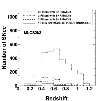
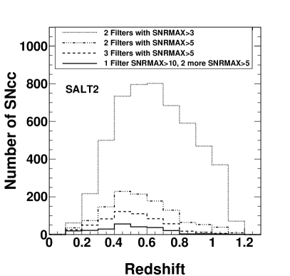
In this appendix we present several supplementary figures; each one is meant to complete the set of SNR cuts shown in plots earlier in the paper. The figure captions should be self-explanatory.
References
- [1] J. P. Bernstein et. al., Supernova Simulations and Strategies For the Dark Energy Survey, ArXiv e-prints (Nov., 2011) [arXiv:1111.1969].
- [2] P. A. Abell et. al., LSST Science Book, Version 2.0, ArXiv e-prints (Dec., 2009) [arXiv:0912.0201].
- [3] A. G. Riess et. al., Observational Evidence from Supernovae for an Accelerating Universe and a Cosmological Constant, AJ 116 (Sept., 1998) 1009–1038, [astro-ph/9805201].
- [4] S. Perlmutter et. al., Measurements of Omega and Lambda from 42 High-Redshift Supernovae, ApJ 517 (June, 1999) 565–586, [astro-ph/9812133].
- [5] R. Kessler et. al., Results from the Supernova Photometric Classification Challenge, PASP 122 (Dec., 2010) 1415–1431, [arXiv:1008.1024].
- [6] S. Jha, A. G. Riess, and R. P. Kirshner, Improved Distances to Type Ia Supernovae with Multicolor Light-Curve Shapes: MLCS2k2, ApJ 659 (Apr., 2007) 122–148, [astro-ph/0612666].
- [7] J. Marriner et. al., A More General Model for the Intrinsic Scatter in Type Ia Supernova Distance Moduli, ApJ 740 (Oct., 2011) 72, [arXiv:1107.4631].
- [8] A. Albrecht et. al., Report of the Dark Energy Task Force, e-prints arXiv:0609591 (Sept., 2006) [astro-ph/0609591].
- [9] R. Kessler et. al., SNANA: A Public Software Package for Supernova Analysis, PASP 121 (Sept., 2009) 1028–1035, [arXiv:0908.4280].
- [10] W. Li et. al., Nearby supernova rates from the Lick Observatory Supernova Search - II. The observed luminosity functions and fractions of supernovae in a complete sample, MNRAS 412 (Apr., 2011) 1441–1472, [arXiv:1006.4612].
- [11] S. J. Smartt et. al., The death of massive stars - I. Observational constraints on the progenitors of Type II-P supernovae, MNRAS 395 (May, 2009) 1409–1437, [arXiv:0809.0403].
- [12] D. Richardson et. al., A Comparative Study of the Absolute Magnitude Distributions of Supernovae, AJ 123 (Feb., 2002) 745–752, [astro-ph/0112051].
- [13] M. Chevallier and D. Polarski, Accelerating Universes with Scaling Dark Matter, International Journal of Modern Physics D 10 (2001) 213–223, [astro-ph/0009008].
- [14] E. V. Linder, Exploring the Expansion History of the Universe, Physical Review Letters 90 (Mar., 2003) 091301, [astro-ph/0208512].