CFTP/12-004

PCCF RI 12-03

Revisiting the $\Gamma\left(K\rightarrow e\nu\right)/\Gamma\left(K\rightarrow\mu\nu\right)$ ratio in

supersymmetric unified models

Renato M. Fonseca^a, J. C. Romão^a and A. M. Teixeira^b

^a Centro de Física Teórica de Partículas, CFTP, Instituto Superior Técnico,

Universidade Técnica de Lisboa, Av. Rovisco Pais 1, 1049-001 Lisboa, Portugal

^b Laboratoire de Physique Corpusculaire, CNRS/IN2P3 – UMR 6533,

Campus des Cézeaux, 24 Av. des Landais, F-63171 Aubière Cedex, France

It has been pointed out that supersymmetric extensions of the Standard Model can induce significant changes to the theoretical prediction of the ratio $\Gamma\left(K\rightarrow e\nu\right)/\Gamma\left(K\rightarrow\mu\nu\right)\equiv R_{K}$, through lepton flavour violating couplings. In this work we carry out a full computation of all one-loop corrections to the relevant $\nu\ell H^{+}$ vertex, and discuss the new contributions to $R_{K}$ arising in the context of different constrained (minimal supergravity inspired) models which succeed in accounting for neutrino data, further considering the possibility of accommodating a near future observation of a $\mu\to e\gamma$ transition. We also re-evaluate the prospects for $R_{K}$ in the framework of unconstrained supersymmetric models. In all cases, we address the question of whether it is possible to saturate the current experimental sensitivity on $R_{K}$ while in agreement with the recent limits on $B$-meson decay observables (in particular BR($B_{s}\to\mu^{+}\mu^{-}$) and BR($B_{u}\to\tau\nu$)), as well as BR($\tau\to e\gamma$) and available collider constraints. Our findings reveal that in view of the recent bounds, and even when enhanced by effective sources of flavour violation in the right-handed $\tilde{e}-\tilde{\tau}$ sector, constrained supersymmetric (seesaw) models typically provide excessively small contributions to $R_{K}$. Larger contributions can be found in more general settings, where the charged Higgs mass can be effectively lowered, and even further enhanced in the unconstrained MSSM. However, our analysis clearly shows that even in this last case SUSY contributions to $R_{K}$ are still unable to saturate the current experimental bounds on this observable, especially due to a strong tension with the $B_{u}\to\tau\nu$ bound.

KEYWORDS: Supersymmetry, neutrinos, meson decays, flavour violation

1 Introduction

Neutrino oscillations have provided the first experimental manifestation of flavour violation in the lepton sector, fuelling the need to consider extensions of the Standard Model (SM) that succeed in explaining the smallness of neutrino masses and the observed pattern of their mixings [1, 2, 3]. In addition to the many facilities dedicated to study neutral leptons, there is currently a great experimental effort to search for signals of flavour violation in the charged lepton sector (cLFV), since such an observation would provide clear evidence for the existence of new physics beyond the SM (trivially extended to accommodate massive neutrinos). The quest for the origin of the underlying mechanism of flavour violation in the lepton sector has been actively pursued in recent years, becoming even more challenging as the MEG experiment is continually improving the sensitivity to $\mu\to e\gamma$ decays [4], thus opening the door for a possible measurement (observation) in the very near future. The current bounds on other radiative decays (i.e. $\ell_{i}\to\ell_{j}\gamma$), or three-body decays ($\ell_{i}\to 3\ell_{j}$) are already impressive [5], and are expected to be further improved in the future.

Supersymmetric (SUSY) extensions of the SM offer new sources of CP and flavour violation, in both quark and lepton sectors. Given the strong experimental constraints, especially on CP and flavour violating observables involving the strongly interacting sector, phenomenological analyses in general favour the so-called “flavour-blind” mechanisms of SUSY breaking, where universality of the soft breaking terms is assumed at some high energy scale: in these constrained scenarios, the only sources of flavour violation (FV) are the quark and charged lepton Yukawa couplings. In order to accommodate current neutrino data, mechanisms of neutrino mass generation, such as the seesaw (in its different realisations - for a review of the latter, see for instance [6, 7]), are often implemented in the framework of (constrained) SUSY models: in the case of the so-called “SUSY-seesaw”, radiatively induced flavour violation in the slepton sector [8] can provide sizable contributions to cLFV observables. The latter have been extensively studied, both at high- and low-energies, over the past years (see e.g. [9]). Flavour violation can be also incorporated in a more phenomenological approach, where at low-energies new sources of FV are present in the soft SUSY breaking terms. However, these are severely constrained by a large number of observables (see, e.g. [10] and references therein).

In addition to the above mentioned rare lepton decays, leptonic and semi-leptonic meson decays also offer a rich testing ground for cLFV. Here we will be particularly interested in leptonic $K$ decays, which (as is also the case of leptonic $\pi$ decays) constitute very good probes of violation of lepton universality. The potential of these observables, especially regarding SUSY extensions of the SM, was firstly noticed in [11], and later investigated in greater detail in [12, 13, 14].

By themselves, these decays are heavily hampered by hadronic uncertainties and, in order to reduce the latter (and render these decays an efficient probe of new physics), one usually considers the ratio

$$R_{K}\,\equiv\,\frac{\Gamma\left(K^{+}\rightarrow e^{+}\nu\left[\gamma\right]\right)}{\Gamma\left(K^{+}\rightarrow\mu^{+}\nu\left[\gamma\right]\right)}\,,$$ (1.1)

since in this case the hadronic uncertainties cancel to a very good approximation. As a consequence, the SM prediction can be computed with high precision [15, 16, 17]. The most recent analysis has provided the following value [17]:

$$R_{K}^{\textrm{SM}}=(2.477\pm 0.001)\times 10^{-5}\,.$$ (1.2)

On the experimental side, the NA62 collaboration has recently obtained very stringent bounds [18]:

$$R_{K}^{\textrm{exp}}\,=\,(2.488\pm 0.010)\,\times 10^{-5}\,,$$ (1.3)

which should be compared with the SM prediction (Eq. (1.2)). In order to do so, it is often useful to introduce the following parametrisation,

$$R_{K}^{\textrm{exp}}\,=\,R_{K}^{\textrm{SM}}\left(1+\Delta r\right)\,,\quad\quad\Delta r\equiv\nicefrac{{R_{K}}}{{R_{K}^{\textrm{SM}}}}-1\,,$$ (1.4)

where $\Delta r$ is a quantity denoting potential contributions arising from scenarios of new physics (NP). Comparing the theoretical SM prediction to the current bounds (i.e., Eqs. (1.2, 1.3)), one verifies that observation is compatible with the SM (at 1$\sigma$) for

$$\Delta r\,=\,\left(4\pm 4\right)\times 10^{-3}\,.$$ (1.5)

Previous analyses have investigated supersymmetric contributions to $R_{K}$ in different frameworks, as for instance low-energy SUSY extensions of the SM (i.e. the unconstrained Minimal Supersymmetric Standard Model (MSSM)) [11, 12, 14], or non-minimal grand unified models (where higher dimensional terms contribute to fermion masses) [13]. These studies have also considered the interplay of $R_{K}$ with other important low-energy flavour observables, magnetic and electric lepton moments and potential implications for leptonic CP violation. Distinct computations, based on an approximate parametrisation of flavour violating effects - the Mass Insertion Approximation (MIA) [19] - allowed to establish that SUSY LFV contributions can induce large contributions to the breaking of lepton universality, as parametrised by $\Delta r$. The dominant FV contributions are in general associated to charged-Higgs mediated processes, being enhanced due to non-holomorphic effects - the so-called “HRS” mechanism [20] -, and require flavour violation in the $RR$ block of the charged slepton mass matrix. It is important to notice that these Higgs contributions have been known to have an impact on numerous observables, and can become especially relevant for the large $\tan\beta$ regime [21, 20, 22, 23, 24, 25, 26, 27, 28, 29, 30, 31].

In the present work, we re-evaluate the potential of a broad class of supersymmetric extensions of the SM to saturate the current measurement of $R_{K}$. Contrary to previous studies, we conduct a full computation of the one-loop corrections to the $\nu\ell H^{+}$ vertex, taking into account the important contributions from non-holormophic effective Higgs-mediated interactions. When possible we establish a bridge between our results and approximate analytical expressions in the literature, and we stress the potential enhancements to the total SUSY contributions. In our numerical analysis we re-investigate the prospects regarding $R_{K}$ of a constrained MSSM onto which several seesaw realisations are embedded (type I [32] and II [33], as well as the inverse seesaw [34]), also briefly addressing $L$–$R$ symmetric models [35, 36]. We then consider more relaxed scenarios, such as non-universal Higgs mass (NUHM) models at high-scale (which are known to enhance this class of observables [13] due to potentially lighter charged Higgs boson masses), and discuss the general prospects of unconstrained low-energy SUSY models. In all cases, we revisit the $R_{K}$ observable in the light of new experimental data: in addition to LHC bounds on the sparticle spectrum [38] and a number of low-energy flavour-related bounds [5, 4], we implement the very recent LHCb results concerning the BR($B_{s}\to\mu^{+}\mu^{-}$) [39]. As we discuss here, the increasing tension with low-energy observables, in particular with $B_{u}\to\tau\nu$, precludes sizable SUSY contributions to $R_{K}$ even in the context of otherwise favoured candidate models as is the case of semi-constrained and unconstrained SUSY models.

This document is organised as follows. Section 2 is devoted to the computation of the 1-loop MSSM prediction for $R_{K}$. We compare our (full) result to the approximations in the literature by means of the mass insertion approximation (among other simplifications), and discuss the dominant sources of flavour violation, and the implications to other observables. Our results for a number of models are collected in Section 3. Further discussion and concluding remarks are given in Section 4. In the Appendices, we detail the computation of the renormalised charged lepton - neutrino - charged Higgs vertex, and summarise the key features of two supersymmetric seesaw realisations (types I and II) used in the numerical analysis.

2 Supersymmetric contributions to $R_{K}$

In the SM, the decay widths of pseudoscalar mesons into light leptons are given by

$$\Gamma^{\text{SM}}(P^{\pm}\!\!\to\ell^{\pm}\nu)=\frac{G_{F}^{2}m_{P}m_{\ell}^{2}}{8\pi}\left(\!1-\!\frac{m_{\ell}^{2}}{m_{P}^{2}}\right)^{2}\!\!f_{P}^{2}|V_{qq^{\prime}}|^{2},$$ (2.1)

where $P$ denotes $\pi,K,D$ or $B$ mesons, with mass $m_{P}$ and decay constant $f_{P}$, and where $G_{F}$ is the Fermi constant, $m_{\ell}$ the lepton mass and $V_{qq^{\prime}}$ the corresponding Cabibbo-Kobayashi-Maskawa (CKM) matrix element. These decays are helicity suppressed (as can be seen from the factor $m_{\ell}^{2}$ in Eq. (2.1)), and the prediction for their amplitude is thus hampered by the hadronic uncertainties in the meson decay constants. As mentioned in the Introduction, ratios of these amplitudes are independent of $f_{P}$ to a very good approximation, and the SM prediction can then be computed very precisely. Concerning the kaon decay ratio $R_{K}$, the SM prediction (inclusive of internal bremsstrahlung radiation) is [17]

$$R_{K}^{\text{SM}}\,=\,\left(\frac{m_{e}}{m_{\mu}}\right)^{2}\,\left(\frac{m_{K}^{2}-m_{e}^{2}}{m_{K}^{2}-m_{\mu}^{2}}\right)^{2}\,\left(1+\delta R_{\text{QED}}\right)\,,$$ (2.2)

where $\delta R_{\text{QED}}$ is a small electromagnetic correction accounting for internal bremsstrahlung and structure-dependent effects ($\delta R_{\text{QED}}=(-3.60\pm 0.04)\%$ [17]).

Figure 1: Tree level contributions to $R_{K}$ - SM and charged Higgs.

In supersymmetric models, the extended Higgs sector can play an important rôle in lepton flavour violating transitions and decays (see [21, 20, 22, 23, 24, 25, 26, 27, 28, 29, 30, 31]). The effects of the additional Higgs are also sizable in meson decays through a charged Higgs boson, as schematically depicted in Fig. 1. In particular, for kaons, one finds [21]

$$\Gamma(K^{\pm}\to\ell^{\pm}\nu)\,= \,\Gamma^{\text{SM}}(K^{\pm}\to\ell^{\pm}\nu)$$

$$\times\left(1-\tan^{2}\beta\,\frac{m_{K}^{2}}{m_{H^{+}}^{2}}\,\frac{m_{s}}{m_{s}+m_{u}}\right)^{2};$$ (2.3)

however, despite this new tree-level contribution, $R_{K}$ is unaffected, as the extra factor does not depend on the (flavoured) leptonic part of the process.

New contributions to $R_{K}$ only emerge at higher order: at one-loop level, there are box and vertex contributions, wave function renormalisation, which can be both lepton flavour conserving (LFC) and lepton flavour violating. Flavour conserving contributions arise from loop corrections to the $W^{\pm}$ propagator, through heavy Higgs exchange (neutral or charged) as well as from chargino/neutralino-sleptons (in the latter case stemming from non-universal slepton masses, i.e., a selectron-smuon mass splitting). As concluded in [11], in the framework of SUSY models where lepton flavour is conserved, the new contributions to $\Delta r^{\text{SUSY}}$ are too small to be within experimental reach.

On the other hand, Higgs mediated LFV processes are capable of providing an important contribution when the kaon decays into a electron plus a tau-neutrino. For such LFV Higgs couplings to arise, the leptonic doublet ($L$) must couple to more than one Higgs doublet. However, at tree level in the MSSM, $L$ can only couple to $H_{1}$, and therefore such LFV Higgs couplings arise only at loop level, due to the generation of an effective non-holomorphic coupling between $L$ and $H_{2}^{*}$ - the HRS mechanism [20] - which is a crucial ingredient in enhancing the Higgs contributions to LFV observables. In what follows, we address the impact of these non-holomorphic terms for $R_{K}$.

2.1 LFV Higgs mediated contributions to $R_{K}$

We consider as starting point the MSSM, defined by its superpotential and soft-SUSY breaking Lagrangian. We detail below the relevant terms for our discussion:

$$\mathcal{W}=\hat{U}^{c}Y^{u}\hat{Q}\hat{H}_{2}-\hat{D}^{c}Y^{d}\hat{Q}\hat{H}_{1}-\hat{E}^{c}Y^{l}\hat{L}\hat{H}_{1}-\mu\hat{H}_{1}\hat{H}_{2},$$ (2.4)

$$\mathcal{V}_{\text{soft}}= -\mathcal{L}_{\text{soft}}\,=(M_{\alpha}\,\psi_{\alpha}\,\psi_{\alpha}+\text{h.c.})+m_{H_{i}}^{2}\,H_{i}^{*}\,H_{i}$$

$$+(B\,H_{1}\,H_{2}+\text{h.c.})+\tilde{\ell}_{L}^{*}\,m_{\tilde{L}}^{2}\,\tilde{\ell}_{L}\,+\tilde{\ell}_{R}^{*}\,m_{\tilde{R}}^{2}\tilde{\ell}_{R}\,$$

$$+\,(H_{1}\,\tilde{\ell}_{R}^{*}\,A^{l}\,\tilde{\ell}_{L}\,+\text{h.c.})+...\,,$$ (2.5)

where $M_{\alpha}$ denotes the soft-gaugino mass terms, “…” stand for the squark terms, and we have omitted flavour indices. For the SU(2) superfield products, we adopt the convention $\hat{H}_{1}\,\hat{H}_{2}\equiv\hat{H}_{1}^{1}\,\hat{H}_{2}^{2}-\hat{H}_{1}^{2}\,\hat{H}_{2}^{1}$ (and likewise for similar cases).

From an effective theory approach, the HRS mechanism can be accounted for by additional terms, corresponding to the higher-order corrections to the Higgs-neutrino-charged lepton interaction (schematically depicted in Fig. 2).

Figure 2: Corrections to the $\nu\ell H^{+}$ vertex, as discussed in the text.

At tree-level, the Lagrangian describing the $\nu\ell H^{\pm}$ interaction is given by

$$\mathcal{L}_{0}^{H^{\pm}}\,= \,\overline{\nu}_{L}\,Y^{l\dagger}\,\ell_{R}\,H_{1}^{-*}+\textrm{h.c.}\,$$

$$= \,\left(2^{3/4}\,G_{F}^{1/2}\right)\,\tan\beta\,\overline{\nu}_{L}\,M^{l}\,\ell_{R}\,H^{+}+\textrm{h.c.}\,,$$ (2.6)

with $M^{l}=\textrm{diag}\left(m_{e},m_{\mu},m_{\tau}\right)$. At loop level, two new terms are generated: $\overline{\nu}_{L}\Delta^{+}\ell_{R}H_{2}^{+}-\overline{\ell}_{L}\Delta^{0}\ell_{R}H_{2}^{0}+\textrm{h.c.}$. The second one, with $\Delta^{0}$, forces a redefinition of the charged lepton Yukawa couplings, $Y^{l\dagger}=\frac{M^{l}}{v_{1}}$ $\to$ $Y^{l\dagger}\approx\frac{M^{l}}{v_{1}}-\Delta^{0}\tan\beta$, which in turn implies a redefinition of the charged lepton propagator; the term with $\Delta^{+}$ corrects the Higgs-neutrino-charged lepton vertex. Once these terms are taken into account, the interaction Lagrangian, Eq. (2.6), becomes

$$\mathcal{L}^{H^{\pm}} \,=\,\left(2^{3/4}\,G_{F}^{1/2}\right)\,\tan\beta\,\,\overline{\nu}_{L}\,M^{l}\,\ell_{R}\,H^{+}\,$$

$$+\,\cos\beta\,\,\overline{\nu}_{L}\,\left(\Delta^{+}-\Delta^{0}\,\tan^{2}\beta\right)\,\ell_{R}\,H^{+}+\textrm{h.c.}\,.$$ (2.7)

Since in the $\textrm{SU(2)}_{L}$-preserving limit $\Delta^{+}=\Delta^{0}$, it is reasonable to assume that, after electroweak (EW) symmetry breaking, both terms remain approximately of the same order of magnitude. Hence, it is clear that the contribution associated with $\Delta^{0}$ (the loop contribution to the charged lepton mass term) will be enhanced by a a factor of $\tan^{2}\beta$ when compared to the one associated with $\Delta^{+}$. This simple discussion allows to understand the origin of the dominant SUSY contribution to $R_{K}$.

As we proceed to discuss, a quantitative assessment of the corrections to $\Delta^{+}$ and $\Delta^{0}$ requires considering the higher-order effects on the vertex $\overline{\nu}_{L}\,Z^{H}\,\ell_{R}\,H^{+}$ (see also [41]). The $Z^{H}$ matrix depends on the following (loop-induced) quantities:

• $\eta_{L}^{\ell}$ and $\eta_{L}^{\nu}$ (corrections to the kinetic terms of $\ell_{L}$ and $\nu_{L}$);

• $\eta_{m}^{\ell}$ (correction to the charged lepton mass term);

• $\eta^{H}$ (correction to the $\nu\ell H$ vertex).

The expressions for the distinct $\eta$-parameters can be found in Appendix A. Instead of $Z^{H}$, which includes both tree and loop level effects, it proves to be more convenient to use the following combination,

$$-\frac{\tan\beta}{2^{3/4}G_{F}^{1/2}}\,\left(\frac{m_{K}}{m_{H^{+}}}\right)^{2}\,\frac{m_{s}}{m_{s}+m_{u}}\,Z^{H}\,\left(M^{l}\right)^{-1}\,\equiv\,\epsilon\,\mathbf{1}+\Delta\,,$$ (2.8)

where

$$\epsilon =-\tan^{2}\beta\,\left(\frac{m_{K}}{m_{H^{+}}}\right)^{2}\frac{m_{s}}{m_{s}+m_{u}}\,,$$ (2.9)

$$\Delta =\epsilon\,\left[\frac{\eta_{L}^{\ell}}{2}-\frac{\eta_{L}^{\nu}}{2}+\left(\frac{\eta^{H}}{2^{3/4}\,G_{F}^{1/2}\tan\beta}-\eta_{m}^{\ell}\right)\left(M^{l}\right)^{-1}\right].$$ (2.10)

In the above, $\epsilon$ encodes the tree level Higgs mediated amplitude (which does not change the SM prediction for $R_{K}$), while $\Delta$, a matrix in lepton flavour space, encodes the 1-loop effects. The main contribution is expected to arise from $\eta_{m}^{\ell}$.

The $\Delta r$ observable is then related to $\epsilon$ and $\Delta$ as follows:

$$\Delta r\equiv\frac{R_{K}}{R_{K}^{\text{SM}}}-1\,=\,\frac{\left[\left(\mathbf{1}+\frac{\Delta^{\dagger}}{1+\epsilon}\right)\left(\mathbf{1}+\frac{\Delta}{1+\epsilon}\right)\right]_{ee}}{\left[\left(\mathbf{1}+\frac{\Delta^{\dagger}}{1+\epsilon}\right)\left(\mathbf{1}+\frac{\Delta}{1+\epsilon}\right)\right]_{\mu\mu}}-1\,.$$ (2.11)

If the slepton mixing is sufficiently large, this expression can be approximated as

$$\Delta r\,\approx\,2\,\operatorname{Re}(\Delta_{ee})\,+\,(\Delta^{\dagger}\Delta)_{ee}\,.$$ (2.12)

In the above, the first (linear) term on the right hand-side is due to an interference with the SM process, and is thus lepton flavour conserving. As shown in [11], this contribution can be enhanced through both large $RR$ and $LL$ slepton mixing. On the other hand, the quadratic term $(\Delta^{\dagger}\Delta)_{ee}$ can be augmented mainly through a large LFV contribution from $\Delta_{\tau e}$, which can only be obtained in the presence of significant $RR$ slepton mixing.

2.2 Generating $\Delta r$: sources of flavour violation and experimental constraints

In order to understand the dependence of $\Delta r$ on the SUSY parameters, and the origin of the dominant contributions to this observable, an approximate expression for $\Delta$ is required. Firstly, we notice that the previous discussion, leading to Eq. (2.7), suggests that the $\eta_{m}^{\ell}$ term is responsible for the dominant contributions to $\Delta r$. Thus, in what follows, and for the purpose of obtaining simple analytical expressions, we shall neglect the contributions of the other terms (although these are included in the numerical analysis of Section 3). A fairly simple analytical insight can be obtained when working in the limit in which the virtual particles in the loops (sleptons and gauginos) are assumed to have similar masses, so that their relative mass splittings are indeed small. In this limit, one can Taylor-expand the loop functions entering $\eta_{m}^{\ell}$ (see Appendix A); working to third order in this expansion, and keeping only the terms enhanced by a factor of $m_{\tau}\,\tan\beta\,\frac{m_{\text{SUSY}}}{m_{\text{EW}}}$ (where $m_{\text{SUSY}},\,m_{\text{EW}}$ denote the SUSY breaking scale and EW scale, respectively), we obtain

$$\Delta r\,\sim\, \left[1+X\left(1-\frac{9}{10}\frac{\delta}{\overline{m}_{\widetilde{\ell},\chi^{0}}^{2}}\right)\left(m_{\tilde{L}}^{2}\right)_{e\tau}\right]^{2}-1$$

$$+X^{2}\left[-\mu^{2}+\delta\left(3-\frac{3}{10}\frac{\mu^{2}+2M_{1}^{2}}{\overline{m}_{\widetilde{\ell},\chi^{0}}^{2}}\right)\right]^{2},$$ (2.13)

where $\mu$, $M_{1}$ and $(m_{\tilde{L}}^{2})_{e\tau}$ denote the low-energy values of the Higgs bilinear term, bino soft-breaking mass, and off-diagonal entry of the soft-breaking left-handed slepton mass matrix, respectively. We have also introduced $\overline{m}_{\widetilde{\ell},\chi^{0}}^{2}=\frac{1}{2}(\langle{m}_{\widetilde{\ell}}^{2}\rangle+\langle{m}_{\chi^{0}}^{2}\rangle)$, the average mass squared of sleptons and neutralinos ($\approx m^{2}_{\text{SUSY}}$), and $\delta=\frac{1}{2}(\langle{m}_{\widetilde{\ell}}^{2}\rangle-\langle{m}_{\chi^{0}}^{2}\rangle)$, the corresponding splitting. The quantity $X$ is given by

$$X\,\equiv\,\frac{1}{192\pi^{2}}\,m_{K}^{2}\,g^{\prime 2}\,\mu\,M_{1}\,\frac{\tan^{3}\beta}{m_{H^{+}}^{2}}\,\frac{m_{\tau}}{m_{e}}\,\frac{\left(m_{\tilde{R}}^{2}\right)_{\tau e}}{(\overline{m}_{\widetilde{\ell},\chi^{0}}^{2})^{3}}\,,$$ (2.14)

and it illustrates in a transparent (albeit approximate) way the origin of the terms contributing to the enhancement of $R_{K}$: in addition to the factor ${\tan^{3}\beta}/{m_{H^{+}}^{2}}$, usually associated with Higgs exchanges, the crucial flavour violating source emerges from the off-diagonal $(\tau e)$ entry of the right-handed slepton soft-breaking mass matrix.

Using the above analytical approximation, one easily recovers the results in the literature, usually obtained using the MIA. For instance, Eq. (11) of Ref. [11] amounts to

$$\Delta r\,\sim\,2X\,\left(m_{\tilde{L}}^{2}\right)_{e\tau}\,+\,X^{2}\,\left(m_{\tilde{L}}^{2}\right)_{e\tau}^{2}\,+\,X^{2}\,\delta^{2}\,,$$ (2.15)

which stems from having kept the dominant (crucial) second and third order contributions in the expansion: $X^{2}\delta^{2}$ and $2X\left(m_{\tilde{L}}^{2}\right)_{e\tau}+X^{2}\left(m_{\tilde{L}}^{2}\right)_{e\tau}^{2}$, respectively.

Regardless of the approximation considered, it is thus clear that the LFV effects on kaon decays into a $e\nu$ or $\mu\nu$ pair can be enhanced in the large $\tan\beta$ regime (especially in the presence of low values of $m_{H^{+}}$), and via a large $RR$ slepton mixing $\left(m_{\tilde{R}}^{2}\right)_{\tau e}$. Although the latter is indeed the privileged source, notice that, as can be seen from Eq. (2.15), a strong enhancement can be obtained from sizable flavour violating entries of the left-handed slepton soft-breaking mass, $\left(m_{\tilde{L}}^{2}\right)_{e\tau}$. This is in fact a globally flavour conserving effect (which can also account for negative contributions to $R_{K}$). Previous experimental measurements of $R_{K}$ appeared to favour values smaller than the SM theoretical estimation, thus motivating the study of regimes leading to negative values of $\Delta r$ [11], but these regimes have now become disfavoured in view of the present bounds, Eq. (1.5).

Clearly, these Higgs mediated exchanges, as well as the FV terms at the origin of the strong enhancement to $R_{K}$, will have an impact on a number of other low-energy observables, as can be easily inferred from the structure of Eqs. (2.13-2.15). This has been extensively addressed in the literature [11, 12, 13, 14], and here we will only briefly discuss the most relevant observables: electroweak precision data on the anomalous electric and magnetic moments of the electron, as well as the naturalness of the electron mass, directly constrain the $\eta_{m}^{\ell}$ corrections (and $\eta_{L}^{\ell}$, $\eta^{H}$); low-energy cLFV observables, such as $\tau\to\ell\gamma$ and $\tau\to 3\ell$ decays are also extremely sensitive probes of Higgs mediated exchanges, and in the case of $\tau-e$ transitions, depend on the same flavour violating entries. It has been suggested that positive and negative values of $\Delta r$ can be of the order of 1%, still in agreement with data on the electron’s electric dipole moment and on $\tau\rightarrow\ell\gamma$ [11, 12, 13]. Finally, other meson decays, such as $B\to\ell\ell$ (and $B\to\ell\nu$), exhibit a similar dependence on $\tan\beta$, $\tan^{n}\beta/{m_{H^{+}}}^{4}$ [42] ($n$ ranging from 2 to 6, depending on the other SUSY parameters), and may also lead to indirect bounds on $\Delta r$. In particular, the strict bounds on BR($B_{u}\to\tau\nu$) [5] and the very recent limits on BR($B_{s}\to\mu^{+}\mu^{-}$) [39] might severely constrain the allowed regions in SUSY parameter space for large $\tan\beta$. Although we will come to this issue in greater detail when discussing the numerical results, it is clear that the similar nature of the $K^{+}\to\ell\nu$ and $B_{u}\to\tau\nu$ processes (easily inferred from a generalization of Eq. (2.3), see e.g. [21, 43]) will lead to a tension when light charged Higgs masses are considered to saturate the bounds on $R_{K}$.

Supersymmetric models of neutrino mass generation (such as the SUSY seesaw) naturally induce sizable cLFV contributions, via radiatively generated off-diagonal terms in the $LL$ (and to a lesser extent $LR$) slepton soft-breaking mass matrices [8]. In addition to explaining neutrino masses and mixings, such models can also easily account for values of BR($\mu\to e\gamma$), within the reach of the MEG experiment. In view of the recent confirmation of a large value for the Chooz angle ($\theta_{13}\sim 8.8^{\circ}$) [3] and on the impact it might have on $(m_{\tilde{L}}^{2})_{e\tau}$, in the numerical analysis of the following section we will also consider different realisations of the SUSY seesaw (type I [32], II [33] and inverse [34]), embedded in the framework of constrained SUSY models. We will also revisit semi-constrained scenarios allowing for light values of $m_{H^{+}}$, re-evaluating the predictions for $R_{K}$ under a full, one loop-computation, and in view of recent experimental data. Finally, we confront these (semi-)constrained scenarios with general, low-energy realisations, of the MSSM.

3 Prospects for $R_{K}$: unified vs unconstrained SUSY models

In this section we evaluate the SUSY contributions to $R_{K}$, with the results obtained via the full expressions for $\Delta r$, as described in Section 2. These were implemented into the SPheno public code [44], which was accordingly modified to allow the different studies. It is important to stress that although some approximations have still been done (as previously discussed), the results based on the present computation strongly improve upon those so far reported in the literature (mostly obtained using the MIA). Although the different contributions cannot be easily disentangled due to having carried a full computation, our results automatically include all one-loop lepton flavour violating and lepton flavour conserving contributions (in association with charged Higgs mediation, see footnote 3). As mentioned before, we evaluate $R_{K}$ in the framework of constrained, semi-constrained (NUHM) and unconstrained SUSY models. Concerning the first two, we assume some flavour blind mechanism of SUSY breaking (for instance minimal supergravity (mSUGRA) inspired), so that the soft breaking parameters obey universality conditions at some high-energy scale, which we choose to be the gauge coupling unification scale $M_{\text{GUT}}\sim 10^{16}$ GeV,

$$\left(m_{\tilde{Q}}\right)_{ij}^{2}\,= \,\left(m_{\tilde{U}}\right)_{ij}^{2}\,=\,\left(m_{\tilde{D}}\right)_{ij}^{2}\,=\,\left(m_{\tilde{L}}\right)_{ij}^{2}\,=\,\left(m_{\tilde{R}}\right)_{ij}^{2}$$

$$= \,m_{0}^{2}\,\delta_{ij}\,,\,\,$$

$$\left(A^{l}\right)_{ij}\,= \,A_{0}\,(Y^{l})_{ij}\,.$$ (3.1)

In the above, $m_{0}$ and $A_{0}$ are the universal scalar soft-breaking mass and trilinear couplings of the cMSSM, and $i,j$ denote lepton flavour indices ($i,j=1,2,3$). In the latter case, the gaugino masses are also assumed to be universal, their common value being denoted by $M_{1/2}$. We will also consider the supersymmetrisation of several mechanisms for neutrino mass generation. More specifically, we have considered the type I and type II SUSY seesaw (as detailed in Appendix B). We briefly comment on the inverse SUSY seesaw, and discuss a $L-R$ model.

The strict universality boundary conditions of Eqs. (3.1) will be relaxed for the Higgs sector when we address NUHM scenarios, so that in the latter case we will have

$$m_{H_{1}}^{2}\,\neq m_{H_{2}}^{2}\,\neq\,m_{0}^{2}\,.$$ (3.2)

All the above universality hypothesis will be further relaxed when, for completeness, and to allow a final comparison with previous analyses, we address the low-energy unconstrained MSSM.

In our numerical analysis, we took into account LHC bounds on the SUSY spectrum [38], as well as the constraints from low-energy flavour dedicated experiments [5], and neutrino data [1, 2]. In particular, concerning lepton flavour violation, we have considered [5, 4]:

$$\text{BR}(\tau\to e\gamma)\,<3.3\times 10^{-8}\,\quad(90\%\text{C.L.})\,,$$ (3.3)

$$\text{BR}(\tau\to 3\,e)\,<2.7\times 10^{-8}\,\quad(90\%\text{C.L.})\,,$$ (3.4)

$$\text{BR}(\mu\to e\gamma)\,<2.4\times 10^{-12}\,\quad(90\%\text{C.L.})\,,$$ (3.5)

$$\text{BR}(B_{u}\to\tau\nu)\,>9.7\times 10^{-5}\,\quad(2\,\sigma)\,.$$ (3.6)

Also relevant are the recent LHCb bounds [39]

$$\text{BR}(B_{s}\to\mu^{+}\mu^{-})\,<4.5\times 10^{-9}\,\quad(95\%\text{C.L.})\,,$$ (3.7)

$$\text{BR}(B\to\mu^{+}\mu^{-})\,<1.03\times 10^{-9}\,\quad(95\%\text{C.L.})\,.$$ (3.8)

When addressing models for neutrino mass generation, we take the following (best-fit) values for the neutrino mixing angles [2] (where $\theta_{13}$ is already in good agreement with the most recent results from [3]),

$$\sin^{2}\theta_{12}\,=\ 0.312_{-0.015}^{+0.017},\quad\sin^{2}\theta_{23}\,=\ 0.52_{-0.07}^{+0.06},$$

$$\sin^{2}\theta_{13}\approx 0.013_{-0.005}^{+0.007}\,,$$ (3.9)

$$\Delta\,m_{\text{12}}^{2}\,=\,(7.59_{-0.18}^{+0.20})\,\times 10^{-5}\,\,\text{eV}^{2}\,,$$ (3.10)

$$\Delta\,m_{\text{13}}^{2}\,=(2.50_{-0.16}^{+0.09})\,\times 10^{-3}\,\,\text{eV}^{2}\,.$$ (3.11)

Regarding the leptonic mixing matrix ($U_{\text{MNS}}$) we adopt the standard parametrisation. In the present analysis, all CP violating phases are set to zero.

3.1 mSUGRA inspired scenarios: cMSSM and the SUSY seesaw

We begin by re-evaluating, through a full computation of the one-loop corrections, the maximal amount of supersymmetric contributions to $R_{K}$ in constrained SUSY scenarios. For a first evaluation of $R_{K}$, we consider different cMSSM (mSUGRA-like) points, defined in Table 1. Among them are several cMSSM benchmark points from [45], representative of low and large $\tan\beta$ regimes, as well as some variations. Notice that, as mentioned before, these choices are compatible with having a Higgs boson mass above 118 GeV but will be excluded once we require $m_{h}$ to lie close to 125 GeV as suggested by LHC results [37].

	$m_{0}$ (GeV)	$M_{1/2}$ (GeV)	$\tan\beta$	$A_{0}$ (GeV)	sign($\mu$)
10.3.1	300	450	10	0	1
P20	330	500	20	-500	1
P30	330	500	30	-500	1
40.1.1	330	500	40	-500	1
40.3.1	1000	350	40	-500	1

Table 1: cMSSM (benchmark) points used in the numerical analysis.

As could be expected from Eqs. (2.13-2.15), in a strict cMSSM scenario (in agreement with the experimental bounds above referred to) the SUSY contributions to $R_{K}$ are extremely small; motivated by the need to accommodate neutrino data, and at the same time accounting for values of BR($\mu\to e\gamma$) within MEG reach, we implement type I and type II seesaws in mSUGRA-inspired models (see Appendices B.1 and B.2). Regarding the heavy-scale mediators, we considered degenerate right-handed neutrinos, as well as degenerate scalar triplets. We set the seesaw scale aiming at maximising the (low-energy) non-diagonal entries of the soft-breaking slepton mass matrices, while still in agreement with the current low-energy bounds (see Eqs. (3.3-3.8)). In particular, we have tried to maximise the $LL$ contributions to $\Delta r$, i.e., $(m_{\tilde{L}}^{2})_{e\tau}$, and to obtain BR($\mu\to e\gamma$) within MEG reach (i.e. $10^{-13}\lesssim$ BR($\mu\to e\gamma$)$\lesssim 2.4\times 10^{-12}$). However, and due to the fact that both seesaw realisations fail to account for radiatively induced LFV in the right-handed slepton sector, one finds values $|\Delta r|\lesssim 2\times 10^{-8}$. It is worth emphasising that if one further requires $m_{h}$ to lie close to 125 GeV (as suggested by recent findings [37]), then one is led to regions in mSUGRA parameter space where, due to the much heavier sparticle masses and typically lower values of $\tan\beta$, the SUSY contributions to $R_{K}$ become even further suppressed.

Thus, and even under a full computation of the corrections to the $\nu\ell H^{+}$ vertex, we nevertheless confirm that, as firstly put forward in the analyses of [11, 12] strictly constrained SUSY and SUSY seesaw models indeed fail to account for values of $R_{K}$ close to the present limits.

Clearly, new sources of flavour violation, associated to the right-handed sector are required: in what follows, we maintain universality of soft-breaking terms allowing, at the grand unified (GUT) scale, for a single $\tau-e$ flavour violating entry in $m_{\tilde{R}}^{2}$. This approach is somewhat closer to the lines of [11, 12, 13, 14], although in our computation we will still conduct a full evaluation of the distinct contributions to $\Delta r$, and we consider otherwise universal soft-breaking terms. Without invoking a specific framework/scenario of SUSY breaking that would account for such a pattern, we thus set

$$\delta_{31}^{RR}\,=\,\frac{(m_{\tilde{R}}^{2})_{\tau e}}{m_{0}^{2}}\,\neq 0\,.$$ (3.12)

As discussed above, low-energy constraints on LFV observables (especially $\tau\rightarrow e\gamma$), severely constrain this entry.

In Fig. 3, we present our results for $\Delta r$ scanning the $m_{0}-M_{1/2}$ plane for a regime of large $\tan\beta$. We have set $\delta_{31}^{RR}=0.1$, $\tan\beta=40$, and taken $A_{0}=-500$ GeV. The surveys displayed in the panels correspond to having embedded a type I (left) or type II (right) seesaw onto this near-mSUGRA framework.

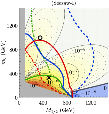
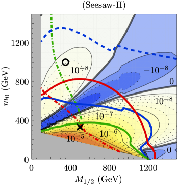
Figure 3: $m_{0}-M_{1/2}$ plane for $\tan\beta=40$ and $A_{0}=-500$ GeV, with $\delta_{31}^{RR}=0.1$. On the left (right) panel, a type I (II) SUSY seesaw, considering degenerate heavy mediators. Contour lines denote values of $\Delta r$ (decreasing values: positive - in association with an orange-yellow-white colour gradient; negative - blue gradients); solid (grey) regions are excluded due to the - requirement of having the correct EWSB. A green dot-dashed line corresponds to the present LHC bounds on the cMSSM [46]. A full green line delimits the BR($\tau\to e\gamma$) exclusion region, while full (dot-dashed) red lines correspond to the bounds on BR($B_{s}\to\mu^{+}\mu^{-}$) (BR($B_{u}\to\tau\nu$)). Finally, the region delimited by blue lines corresponds to having BR($\mu\to e\gamma$) within MEG reach (current bound - solid line, future sensitivity - dashed line). Crosses (circles) correspond to the benchmark point 40.1.1 (40.3.1).

As can be readily seen from Fig. 3, once the constraints from low-energy observables have been applied, in the type I SUSY seesaw, the maximum values for $\Delta r$ are $\mathcal{O}(10^{-7})$, associated to the region with a lighter SUSY spectra (which is in turn disfavoured by a “heavy” light Higgs). Even for the comparatively small non-universality, $\delta_{31}^{RR}=0.1$, a considerable region of the parameter space is excluded due to excessive contributions to BR($B_{u}\to\tau\nu$) and BR($\tau\to e\gamma$), thus precluding the possibility of large values of $\Delta r$. In a regime of large $\tan\beta$, the contributions to BR($B_{s}\to\mu^{+}\mu^{-}$) are also sizable, and the recent LHCb results seem to exclude the regions of the parameter space where one could still have $\Delta r\sim\mathcal{O}(10^{-6,-7})$. The excessive SUSY contributions to BR($B_{s}\to\mu^{+}\mu^{-}$) can be somewhat reduced by adjusting $A_{0}$ (in Fig. 3 we fixed $A_{0}=-500$ GeV) and the values of $\Delta r$ can be slightly augmented by increasing $\delta_{31}^{RR}$; in the latter case, the $\tau\to e\gamma$ bound proves to be the most constraining, and values of $\Delta r$ larger than $\mathcal{O}(10^{-6,-7})$ cannot be obtained in these constrained SUSY seesaw models.

The situation is somewhat different for the type II case: firstly notice that a sizable region in the $m_{0}-M_{1/2}$ plane is associated to negative contributions to $R_{K}$, which are currently disfavoured. In the remaining (allowed) parameter space, the values of $\Delta r$ are slightly smaller than for the type I case: this is a consequence of a non trivial interplay between a smaller value for the splitting $\delta=\frac{1}{2}(\langle{m}_{\widetilde{\ell}}^{2}\rangle-\langle{m}_{\chi^{0}}^{2}\rangle)$ (induced by a lighter spectra), and a lighter charged Higgs boson. (We notice that accommodating light neutral Higgs with $m_{h}>118$ GeV is also comparatively more difficult in the type II SUSY seesaw.)

Notice that in both SUSY seesaws it is fairly easy to accommodate a potential observation of BR($\mu\to e\gamma$) $\sim 10^{-13}$ by MEG, taking for instance $M_{{\rm Seesaw}}\sim 10^{12}$ GeV for the type I and II seesaw mechanisms.

For both cases, larger values of $\delta_{31}^{RR}=0.5$ can be taken, but these typically lead to conflicting situations with low-energy observables; lowering $\tan\beta$ can ease the existing tension, at the expense of also reducing $\Delta r$. We summarise this on Table 2, for simplicity in association with a type I SUSY seesaw.

	$\delta_{31}^{RR}$	$\Delta r$	$m_{H^{+}}$ (GeV)	BR($\tau\to e\gamma$)	BR($B_{u}\to\tau\nu$) $(\times 10^{-4})$	BR($B_{s}\to\mu^{+}\mu^{-}$) $(\times 10^{-9})$	BR($\mu\to e\gamma$)
10.3.1 - I	0	7.2$\times 10^{-11}$	715	2.5$\times 10^{-16}$	1.17	4.0	7.2$\times 10^{-14}$
10.3.1 - I	0.1	8.5$\times 10^{-11}$	715	2.9$\times 10^{-10}$	1.17	4.0	1.8$\times 10^{-13}$
10.3.1 - I	0.5	5.1$\times 10^{-9}$	715	8.5$\times 10^{-9}$	1.12	4.0	9.7$\times 10^{-15}$
P20 - I	0.1	4.3$\times 10^{-9}$	800	3.5$\times 10^{-9}$	1.15	4.0	2.0$\times 10^{-12}$
P30 - I	0.1	1.2$\times 10^{-7}$	725	1.4$\times 10^{-8}$	1.11	4.3	1.7$\times 10^{-14}$
40.3.1 - I	0	1.6$\times 10^{-8}$	818	3.1$\times 10^{-15}$	1.09	4.4	1.2$\times 10^{-12}$
40.3.1 - I	0.1	6.0$\times 10^{-8}$	818	2.9$\times 10^{-10}$	1.09	4.4	1.2$\times 10^{-12}$
40.3.1 - I	0.5	2.0$\times 10^{-6}$	818	2.0$\times 10^{-8}$	1.09	4.4	3.3$\times 10^{-12}$

Table 2: $\Delta r$ and other low-energy observables for different mSUGRA points, considering a type I seesaw, and distinct values of $\delta_{31}^{RR}$. The values of the seesaw scale were varied from $1.3\times 10^{12}$ GeV to $5\times 10^{10}$ GeV, in order to comply with the limits/future sensitivity on BR($\mu\to e\gamma$).

A few comments are in order regarding the summary of Table 2: even with a large value for $\delta_{31}^{RR}$, and in the large $\tan\beta$ regime, the maximum attainable values for $\Delta r$ are much below the current experimental sensitivity, at most $2\times 10^{-6}$. As mentioned before, if we further take into account the recent discovery of a new boson at LHC [37] with a mass around 125 GeV, and interpret it as the lightest neutral CP-even Higgs boson of the MSSM, the attainable values for $\Delta r$ will be extremely small.

In order to conclude this part of the analysis we provide a comprehensive overview of the constrained MSSM prospects regarding $R_{K}$, presenting in Fig. 4 a survey of the (type I seesaw) mSUGRA parameter space, for two different regimes of $\delta_{31}^{RR}$, taking all present bounds (including the recent ones on $m_{h}$) into account. The panels of Fig. 4 allow to recover the information that could be expected from the discussion following Fig. 3: for fixed values of $A_{0}$ and $\tan\beta$, increasing $\delta_{31}^{RR}$ indeed allows to augment the SUSY contributions to $\Delta r$ although, as can be seen from the right-panel, the constraints from BR($\tau\to e\gamma$) become increasingly harder to accommodate. (Notice that the latter could be avoided by increasing the SUSY scale (i.e. on regions of the parameter space with large $m_{0}$ and/or $M_{1/2}$) - however, and as visible from Fig. 4, in a constrained SUSY framework this would lead to heavier charged Higgs masses, and in turn to suppressed contributions to $\Delta r$.)

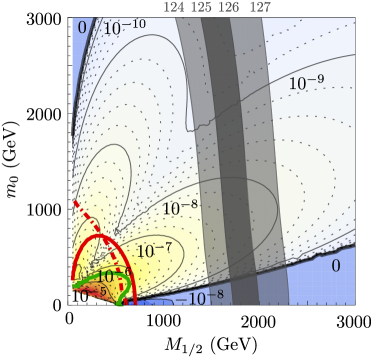
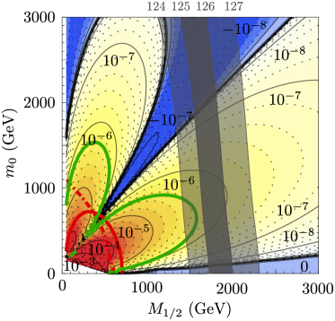
Figure 4: mSUGRA (type I seesaw) $m_{0}-M_{1/2}$ plane for $\tan\beta=40$ and $A_{0}=0$ GeV, with $\delta_{31}^{RR}=0.1$ (left panel) and $\delta_{31}^{RR}=0.7$ (right panel). Contour lines denote values of $\Delta r$ (decreasing values: positive - in association with an orange-yellow-white colour gradient; negative - blue gradients). A full green line delimits the BR($\tau\to e\gamma$) exclusion region, while full (dot-dashed) red lines correspond to the bounds on BR($B_{s}\to\mu^{+}\mu^{-}$) (BR($B_{u}\to\tau\nu$)). Superimposed are the regions for the Higgs boson mass: the dark band is for $125\leq m_{h^{0}}\leq 126$ (GeV) and the lighter one marks the region where $124\leq m_{h^{0}}\leq 127$ (GeV).

Although we do not display an analogous plot here, the situation is very similar for the type II SUSY seesaw (slightly even more constrained due to the fact that accommodating $m_{h}\sim 125$ GeV is more difficult in these models [47]).

In view of the above discussion it is clear that even taking into account all 1-loop corrections to the $\nu\ell H^{+}$ vertex, values of $\Delta r$, large enough to saturate current observation, cannot be reached in the framework of constrained SUSY models (and its seesaw extensions accommodating neutrino data). In this sense, and even though we have followed a different approach, our results follow the conclusions of [13]. We also stress that recent experimental bounds (both from flavour observables and collider searches) add even more severe constraints to the maximal possible values of $\Delta r$.

3.2 mSUGRA inspired scenarios: inverse seesaw and $L-R$ models

We briefly comment here on the prospects of the inverse SUSY seesaw concerning $R_{K}$: recently, it was pointed out that some flavour violating observables can be enhanced by as much as two orders of magnitude in a model with the inverse seesaw mechanism [48]. Within such a framework, right-handed (s)neutrino masses can be relatively light, and as a consequence these ${\nu_{R}}$, ${\widetilde{\nu}_{R}}$ states do not decouple from the theory until the TeV scale, hence potentially providing important contributions to different low-energy processes. Nevertheless, the specific contributions to $\Delta r$ are suppressed by a factor $\frac{m_{e}^{2}}{m_{\tau}^{2}}$, with respect to those discussed above (see Eq. (2.14)), so that we do not expect a significant enhancement of SUSY 1-loop effects to $R_{K}$ due to the inverse seesaw mechanism.

For completeness (and although we do not provide specific details here), we have considered a specific $L-R$ seesaw model [36]. In this framework, non-vanishing values of $\delta_{31}^{RR}$ can be dynamically generated. We have numerically verified that typically one finds $\delta_{31}^{RR}\lesssim 0.01$ (we do not dismiss that larger values might be found, although certainly requiring a considerable amount of fine-tuning in the input parameters). We have not done a dedicated $\Delta r$ calculation for this case, but taking into account that the effect scales with $(\delta_{31}^{RR})^{2}$, we also expect the typical range for $\Delta r$ to be far below the current experimental sensitivity.

3.3 mSUGRA inspired scenarios: NUHM

As can be seen from the approximate expression for $\Delta r$ in Eqs. (2.14, 2.15), regimes associated with both large $\tan\beta$ and a light charged Higgs can greatly enhance this observable [13] ($\Delta r\propto\nicefrac{{\tan^{6}\beta}}{{m_{H^{+}}^{4}}}$). By relaxing the mSUGRA-inspired universality conditions for the Higgs sector, as occurs in NUHM scenarios, one can indeed have very low masses for the $H^{+}$ boson at low energies. This regime corresponds to a narrow strip in parameter space where $m_{H_{1}}^{2}\!\approx\!m_{H_{2}}^{2}$, in particular when both are close to $-(2.2\>\textrm{TeV})^{2}$. In addition to favouring electroweak symmetry breaking, since $m^{2}_{H^{+}}\sim\left|m_{H_{1}}^{2}-m_{H_{2}}^{2}\right|$ (even accounting for RG evolution of the parameters down to the weak scale), it is expected that the charged Higgs can be made very light with some fine tuning [13]. In order to explore the maximal possible values of $\Delta r$, a small scan was conducted around this region, where $m_{H^{+}}$ changes very rapidly (see Table 3).

	$m_{0}$	$M_{1/2}$	$m_{H_{1}}^{2}$, $m_{H_{2}}^{2}$	$\tan\beta$	$\delta_{31}^{RR}$
	(GeV)	(GeV)	$\text{\footnotesize(GeV}^{2}\text{\footnotesize)}$
Min	0	100	$-5.2\times 10^{6}$	40	0.1
Max	1500	1500	$-4.6\times 10^{6}$	40	0.7

Table 3: Range of NUHM parameters leading to the scan of Fig. 5.

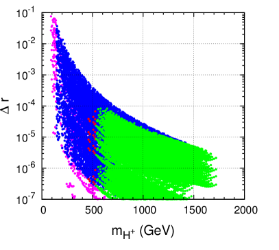
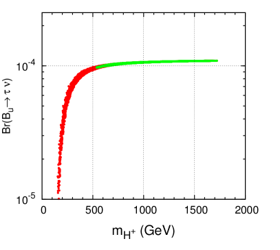
Figure 5: Left panel: $\Delta r$ as a function of the charged Higgs mass, $m_{H^{+}}$ (in GeV). Magenta points have been subject to no cuts, blue points comply with the bounds on the masses (LEP+LHC), red points satisfy all bounds except BR($B_{u}\to\tau\nu$) and green points satisfy all bounds. Right panel: BR($B_{u}\to\tau\nu$) versus $m_{H^{+}}$. Red points satisfy only the bounds on the masses (LEP+LHC) while green points comply with all bounds.

As can be verified from the left-hand panel of Fig. 5, one could in principle have semi-constrained regimes leading to sizable values of $R_{K}$, $\mathcal{O}(10^{-2})$. Once all (collider and low-energy) bounds have been imposed, one has at most $\Delta r\lesssim 10^{-4}$ (in association with $m_{H^{+}}\gtrsim 500$ GeV). Moreover, it is interesting to notice that SUSY contributions to BR($B_{u}\to\tau\nu$), which become non-negligible for lighter $H^{\pm}$, have a negative interference with those of the SM, lowering the latter BR to values below the current experimental bound. This can be seen on the right-hand panel of Fig. 5. We will return to this topic in greater detail in the following subsection, when addressing the unconstrained MSSM.

3.4 Unconstrained MSSM

To conclude the numerical discussion, and to allow for a better comparison between our approach and those usually followed in other recent analyses (for instance [12, 14]), we conduct a final study of the unconstrained, low-energy MSSM. Thus, and in what follows, we make no hypothesis concerning the source of lepton flavour violation, nor on the underlying mechanism of SUSY breaking. Massive neutrinos are introduced by hand (no assumption being made on their nature), and although charged interactions do violate lepton flavour, as parametrised by the $U_{\text{MNS}}$ matrix, no sizable contributions to BR($\mu\to e\gamma$) should be expected, as these would be suppressed by the light neutrino masses. At low-energies, no constraints (other than the relevant experimental bounds) are imposed on the SUSY spectrum (for simplicity, we will assume a common value for all sfermion trilinear couplings at the low-scale, $A_{i}=A_{0}$). The soft-breaking slepton masses are allowed to be non-diagonal, so that a priori a non-negligible mixing in the slepton sector can occur. In order to better correlate the source of flavour violation at the origin of $\Delta r$ with the different experimental bounds, we again allow for a single FV entry in the slepton mass matrices: $\delta_{31}^{RR}\sim 0.5$ (otherwise setting all other $\delta_{ij}^{XY}=0$).

	$\mu$	$m_{A}$	$M_{1}$, $M_{2}$	$M_{3}$	$A_{0}$	$m_{L}$	$m_{R}$	$m_{Q},m_{U},m_{D}$	$\tan\beta$	$\delta_{31}^{RR}$	other $\delta_{ij}^{XY}$
Min	100	50	100	1100	-1000	100	100	1200	30	0.5	0
Max	3000	1500	2500	2500	1000	2200	2500	5000	60	0.5	0

Table 4: Range of variation of the unconstrained MSSM parameters (dimensionful parameters in GeVs). $A_{0}$ denotes the common value of the low-energy sfermion trilinear couplings.

In our scan we have varied the input parameters in the ranges collected in Table 4. We have also applied all relevant constraints on the low-energy observables, Eq. (3.3-3.8), as well as the constraints on the SUSY spectrum [5, 38]. In particular we have assumed the conservative limits

$$m_{\tilde{q}_{L,R}}>1000\,\text{GeV}\,,\quad\quad m_{\tilde{g}}>1000\,\text{GeV}\,.$$ (3.13)

Concerning the light Higgs boson mass, no constraint was explicitly imposed. We just notice here that values close to 125 GeV [37], or even larger, are easily achievable due to the heavy squark masses.

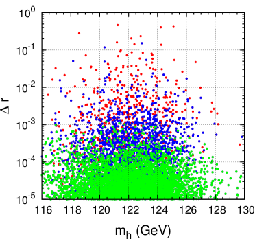
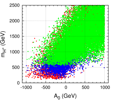
Figure 6: Left panel: $\Delta r$ as a function of the lightest Higgs boson mass $m_{h}$ (in GeV) for the range of parameters shown in Table 4. Red points satisfy the bounds on the spectrum (LEP+LHC), blue points satisfy all bounds except $\textrm{BR}\left(B_{u}\to\tau\nu\right)$ and green points satisfy all bounds. Right panel: $m_{H^{+}}$ versus $A_{0}$ (both in GeV), with the same colour code. Leading to both plots, the different input parameters were varied as in Table 4.

This can be observed from the left panel of Fig. 6, where we display the output of the above scan, presenting the values of $\Delta r$ versus the associated light Higgs boson mass, $m_{h}$. As expected, no explicit correlation between $m_{h}$ and $\Delta r$ is manifest, nor with the other (relevant) flavour-related low-energy bounds. For completeness, and to better illustrate the following discussion, we present on the right-hand panel of Fig. 6 the charged Higgs mass as a function of $A_{0}$, again under a colour scheme denoting the experimental bounds applied in each case. Identical to what was observed in Fig. 5 (notice that NUHM models correspond, at low-energies, to a subset of these general cases), regimes of very light charged Higgs are indeed present, in association with small to moderate (negative) regimes for $A_{0}$. Nevertheless, these regimes - which could potentially enhance $\Delta r$ - are likewise excluded due to a strong conflict with $\textrm{BR}\left(B_{u}\to\tau\nu\right)$. This can be further confirmed from the left panel of Fig. 7, where we display the possible range of variation for $\Delta r$ as a function of $m_{H^{+}}$, colour-coding the different applied bounds.

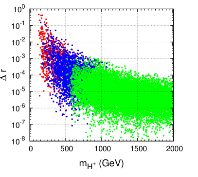
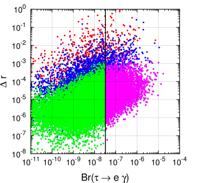
Figure 7: Ranges of variation of $\Delta r$ in the unconstrained MSSM as a function of $m_{H^{+}}$ (left panel), and as a function of BR($\tau\to e\gamma$) (right panel). The different input parameters were varied as in Table 4 (notice that $\delta_{31}^{RR}=0.5$). On the left panel red points satisfy the bounds on the masses (LEP+LHC), blue points satisfy all bounds except $\textrm{BR}\left(B_{u}\to\tau\nu\right)$ and green points comply with all bounds. Similar colour code on the right panel, except that blue points now comply with all bounds except $\textrm{BR}\left(B_{u}\to\tau\nu\right)$ and BR($\tau\to e\gamma$) while magenta denotes points only failing the bound on BR($\tau\to e\gamma$).

As can be seen from both panels of Fig. 7, values $\Delta r\approx\mathcal{O}(10^{-2},10^{-1})$ could be obtainable, in agreement with Refs [14, 11, 12, 13]. However, the situation is substantially altered when one takes into account the current experimental bounds on $B$ decays ($B_{u}\to\tau\nu$ and $B_{s}\to\mu^{+}\mu^{-}$) and $\tau\to e\gamma$. As is manifest from the left panel of Fig. 7, once experimental bounds - other than $B_{u}\to\tau\nu$ - are imposed, one could in principle have $\Delta r^{\text{max}}\approx\mathcal{O}(10^{-2})$; however, taking into account the limits from BR($B_{u}\to\tau\nu$), one is now led to $\Delta r\lesssim 10^{-3}$.

A few comments are in order regarding the impact of the different low-energy bounds from radiative tau decays and $B$-physics observables. Firstly, let us consider the $\tau\to e\gamma$ decay: although directly depending on $\delta_{31}^{RR}$, its amplitude is (roughly) suppressed by the fourth power of the average SUSY scale, $m_{\text{SUSY}}$. As can be seen from Eqs. (2.14, 2.15), $\Delta r$ only depends on the charged Higgs mass - if the latter is assumed to be an EW scale parameter, $\Delta r$ will be thus independent of $m_{\text{SUSY}}$ in these unconstrained models. As such, it is possible to evade the $\tau\to e\gamma$ bound by increasing the soft SUSY masses, and this can indeed be seen from the right-hand panel of Fig. 7, where a number of “blue” points are found to lie below the BR($\tau\to e\gamma$) bound.

Secondly, the $B_{s}\to\mu^{+}\mu^{-}$ decay can be a severe constraint regarding the SUSY contributions to $\Delta r$ in the case of constrained models (see, e.g., Figs. 3 and 4). We notice that $B_{s}\to\mu^{+}\mu^{-}$ is approximately proportional to $A_{0}^{2}$ (see for instance [43]) while $\Delta r$ shows no such dependence: thus a regime of small trilinear couplings easily allows evade the $B_{s}\to\mu^{+}\mu^{-}$ bounds.

Finally, let us discuss the $B_{u}\to\tau\nu$ bounds. Notice that this is a process essentially identical to the charged kaon decays at the origin of the $R_{K}$ ratio (the only difference being that the $K^{+}$ meson is to be replaced by a $B_{u}$ and the $e$/$\mu$ in the decay products by a kinematically allowed $\tau$), and hence its tree-level decay width can be inferred from Eqs. (2.1) and (2.3). Due to a negative interference between the SM and the MSSM contributions, given by the term proportional to $\tan^{2}\beta/m^{2}_{H^{\pm}}$ in Eq. (2.3), regimes of low $m_{H^{+}}$ lead to excessively small values of $B_{u}\to\tau\nu$ (below the experimental bound), effectively setting a lower bound for for $m^{2}_{H^{\pm}}$ (see right panel of Fig. 5, in relation to the discussion of NUHM models). In turn, this excludes regimes of $m_{H^{+}}$ associated to sizable values of $\Delta r$, as is clear from the comparison of the “blue” and “green” regions of the left panel of Fig. 7.

In summary, we conclude that saturating the experimental bound on $R_{K}$ clearly proves to be extremely difficult (if not impossible), even in the unconstrained MSSM, especially in view of the stringent constraints from $B_{u}\to\tau\nu$.

4 Conclusions

In this work we have revisited supersymmetric contributions to $R_{K}=\Gamma\left(K\rightarrow e\nu\right)$$/\Gamma\left(K\rightarrow\mu\nu\right)$, considering the potential of a broad class of constrained SUSY models to saturate the current measurement of $R_{K}$. We based our analysis in a full computation of the one-loop corrections to the $\nu\ell H^{+}$ vertex; we have also derived (when possible) illustrative analytical approximations, which in addition to offering a more transparent understanding of the rôle of the different parameters, also allow to establish a bridge between our results and previous ones in the literature. Our analysis further revisited the $R_{K}$ observable in the light of new experimental data, arising from flavour physics as well as from collider searches.

We numerically evaluated the contributions to $R_{K}$ arising in the context of different minimal supergravity inspired models which account for observed neutrino data, further considering the possibility of accommodating a near future observation of a $\mu\to e\gamma$ decay. As expected from the (mostly) $LL$ nature of the radiatively induced charged lepton flavour violation, type I and II seesaw mechanisms implemented in the cMSSM provide minimal contributions to $R_{K}$, thus implying that such cMSSM SUSY seesaws cannot saturate the present value for $\Delta r$.

We then considered unified models where the flavour-conserving hypothesis on the $RR$ slepton sector is relaxed by allowing a non-vanishing $\delta_{31}^{RR}$ ($e-\tau$ sector). In all models, special attention was given to experimental constraints, especially four observables which turn out to play a particularly relevant rôle: the recent interval for the lightest neutral Higgs boson mass provided by the CMS and ATLAS collaborations, BR($B_{s}\to\mu^{+}\mu^{-}$), BR($B_{u}\to\tau\nu$) and BR($\tau\to e\gamma$). These last two exhibit a dependence on $m_{H^{+}}$ ($B_{u}\to\tau\nu$) and on $\delta_{31}^{RR}$ ($\tau\to e\gamma$) similar to that of $\Delta r$. The SUSY contributions to $\Delta r$ are thus maximised in a regime in which $m_{H^{+}}$ and $\delta_{31}^{RR}$ are such that the experimental limits for $B_{u}\to\tau\nu$ and $\tau\to e\gamma$ are simultaneously saturated; in this regime one must then accommodate the bounds on other observables, such as $m_{h}$ and BR($B_{s}\to\mu^{+}\mu^{-}$). For a minimal deviation from a pure cMSSM scenario allowing for non-vanishing values of $\delta_{31}^{RR}$, we can have values for $\Delta r$ at most of the order of $10^{-6}$. In fact, the requirement of having a Higgs boson mass of 125-126 GeV is much more constraining on the cMSSM parameter space than, for instance $B_{s}\to\mu^{+}\mu^{-}$ (which is sub-dominant, and can be overcome by variations of the trilinear coupling, $A_{0}$). In order to have $\Delta r\sim\mathcal{O}(10^{-6})$, one must significantly increase $\delta_{31}^{RR}$ so to marginally overlap the regions of $m_{h}\sim 125$ GeV, while still in agreement with $\tau\to e\gamma$.

Models where the charged Higgs mass can be significantly lowered, as is the case of NUHM models, allow to increase the SUSY contributions to $\Delta r$, which can be as large as $10^{-4}$ (larger values being precluded due to $B_{u}\to\tau\nu$ decay constraints).

More general models, as the unconstrained MSSM realised at low-energies, offer more degrees of freedom, and the possibility to better accommodate/evade the different experimental constraints. In the unconstrained MSSM, one can find values of $\Delta r$ one order of magnitude larger, $\Delta r\sim\mathcal{O}(10^{-3})$. Again, any further augmentation is precluded due to incompatibility with the bounds on $B_{u}\to\tau\nu$.

However $\Delta r\sim\mathcal{O}(10^{-3})$ still remains one order of magnitude shy of the current experimental sensitivity to $R_{K}$, and also substantially lower than some of the values previously found in the literature. As such, if SUSY is indeed discovered, and unless there is significant progress in the experimental sensitivity to $R_{K}$, it seems unlikely that the contributions to $R_{K}$ of the SUSY models studied here will be testable in the near future. On the other hand, any near-future measurement of $\Delta r$ larger than $\mathcal{O}(10^{-3})$ would unambiguously point towards a scenario different than those here addressed (mSUGRA-like seesaw, NUHM and the phenomenological MSSM).

It should be kept in mind that the analysis presented here focused on the impact of LFV interactions. Should the discrepancy between the SM and experimental observations turn out to be much smaller than $10^{-4}$, a more detailed approach and evaluation will then be necessary.

Appendix A Renormalisation of the $\nu\ell H^{+}$ vertex

In what follows we detail the computation leading to Eqs. (2.8-2.10), and we further refer to [41] for a similar analysis. As expected, loop effects contribute to both kinetic and mass terms of charged leptons as well as to the ${\nu}\ell H^{+}$ vertex:

$$\mathcal{L}_{0}^{H^{\pm}}\!\!= i\,\overline{\ell}_{L}\left(\mathbf{1}+\eta_{L}^{\ell}\right)\not{\partial}\ell_{L}+i\,\overline{\ell}_{R}\left(\mathbf{1}+\eta_{R}^{\ell}\right)\not{\partial}\ell_{R}$$

$$\!\!+i\,\overline{\nu}_{L}\left(\mathbf{1}+\eta_{L}^{\nu}\right)\not{\partial}\nu_{L}-\left[\overline{\ell}_{L}\left(M^{l0}+\eta_{m}^{\ell}\right)\ell_{R}+\textrm{h.c.}\right]$$

$$\!\!+\left[\overline{\nu}_{L}\left(2^{3/4}G_{F}^{1/2}\,\tan\beta\,M^{l0}+\eta^{H}\right)\ell_{R}H^{+}+\textrm{h.c.}\right]\,.$$ (A.1)

Here $M^{l0}$ denotes the bare charged lepton mass and the $\eta$’s correspond to loop contributions to the various terms. The (new) kinetic terms can be recast into a canonical form by means of unitary rotations of the fields ($K_{L}^{\ell}$, $K_{R}^{\ell}$, $K_{L}^{\nu}$), which are then renormalised by diagonal transformations ($\hat{Z}_{L}^{\ell}$, $\hat{Z}_{R}^{\ell}$, $\hat{Z}_{L}^{\nu}$):

$$\ell_{L}^{\text{old}}\!= K_{L}^{\ell}\left(\hat{Z}_{L}^{\ell}\right)^{-\frac{1}{2}}\!\!\ell_{L}^{\text{new}}\ \textrm{;}\quad\hat{Z}_{L}^{\ell}={K_{L}^{\ell}}^{\dagger}\left(\mathbf{1}+\eta_{L}^{\ell}\right)K_{L}^{\ell}\,,$$ (A.2)

$$\ell_{R}^{\text{old}}\!= K_{R}^{\ell}\left(\hat{Z}_{R}^{\ell}\right)^{-\frac{1}{2}}\!\!\ell_{R}^{\text{new}}\ \textrm{;}\quad\hat{Z}_{R}^{\ell}={K_{R}^{\ell}}^{\dagger}\left(\mathbf{1}+\eta_{R}^{\ell}\right)K_{R}^{\ell}\,,$$ (A.3)

$$\nu_{L}^{\text{old}}\!= K_{L}^{\nu}\left(\hat{Z}_{L}^{\nu}\right)^{-\frac{1}{2}}\!\!\nu_{L}^{\text{new}}\ \textrm{;}\quad\hat{Z}_{L}^{\nu}={K_{L}^{\nu}}^{\dagger}\left(\mathbf{1}+\eta_{L}^{\nu}\right)K_{L}^{\nu}\,.$$ (A.4)

Two unitary rotation matrices ($R_{L}^{\ell}$, $R_{R}^{\ell}$) are further required to diagonalise the charged lepton mass matrix, and one finally has

$$\ell_{L}^{\text{old}} = K_{L}^{\ell}\left(\hat{Z}_{L}^{\ell}\right)^{-\frac{1}{2}}\,R_{L}^{\ell}\,\ell_{L}^{\text{new}}\,,$$ (A.5)

$$\ell_{R}^{\text{old}} = K_{R}^{\ell}\left(\hat{Z}_{R}^{\ell}\right)^{-\frac{1}{2}}\,R_{R}^{\ell}\,\ell_{R}^{\text{new}}\,,$$ (A.6)

$$\nu_{L}^{\text{old}} = K_{L}^{\nu}\left(\hat{Z}_{L}^{\nu}\right)^{-\frac{1}{2}}\,R_{L}^{\ell}\,\nu_{L}^{\text{new}}\,.$$ (A.7)

In the new basis, the mass terms now read

$$\mathcal{L}^{\textrm{mass}}\equiv -\overline{\ell}_{L}\,M^{l}\,\ell_{R}+\textrm{h.c.}$$

$$= -\overline{\ell}_{L}\,{R_{L}^{\ell}}^{\dagger}\left[\left(\hat{Z}_{L}^{\ell}\right)^{-\frac{1}{2}}\,{K_{L}^{\ell}}^{\dagger}\left(M^{l0}+\eta_{m}^{\ell}\right)\right.$$

$$\left.\hskip 48.36967ptK_{R}^{\ell}\left(\hat{Z}_{R}^{l}\right)^{-\frac{1}{2}}\right]\,R_{R}^{\ell}\,\ell_{R}+\textrm{h.c.}\,.$$ (A.8)

The above equation relates the unknown parameter $M^{l0}$ with the physical mass matrix $M^{l}$. Using the latter to rewrite the ${\nu}\ell H^{+}$ vertex one finds

$$\mathcal{L}^{H^{\pm}} \equiv \overline{\nu}_{L}\,Z^{H}\,\ell_{R}\,H^{+}+\textrm{h.c.}\,,$$ (A.9)

where

$$Z^{H}= 2^{3/4}G_{F}^{1/2}\,\tan\beta\,{R_{L}^{\ell}}^{\dagger}\left(\hat{Z}_{L}^{\nu}\right)^{-\frac{1}{2}}{K_{L}^{\nu}}^{\dagger}\,K_{L}^{\ell}\left(\hat{Z}_{L}^{\ell}\right)^{\frac{1}{2}}\,R_{L}^{\ell}\,M^{l}$$

$$+{R_{L}^{\ell}}^{\dagger}\left(\hat{Z}_{L}^{\nu}\right)^{-\frac{1}{2}}\,{K_{L}^{\nu}}^{\dagger}\left(-2^{3/4}G_{F}^{1/2}\,\tan\beta\,\eta_{m}^{\ell}+\eta^{H}\right)$$

$$\hskip 14.22636ptK_{R}^{\ell}\left(\hat{Z}_{R}^{\ell}\right)^{-\frac{1}{2}}\,K_{R}^{\ell}\,.$$ (A.10)

To one-loop order, this exact expression simplifies to

$$Z^{H}= 2^{3/4}G_{F}^{1/2}\,\tan\beta\,\left[\left(\mathbf{1}+\frac{\eta_{L}^{\ell}}{2}-\frac{\eta_{L}^{\nu}}{2}\right)\,M^{l}-\eta_{m}^{\ell}\right]+\eta^{H}\,.$$ (A.11)

The expressions for the $\eta$’s can be computed from the relevant Feynman diagrams (assuming zero external momenta):

$$-\left(4\pi\right)^{2}\hskip-2.84526pt \left(\eta_{m}^{\ell}\right)_{ij}=\,N_{i\alpha\beta}^{R\left(\ell\right)}N_{j\alpha\beta}^{L\left(\ell\right)*}m_{\chi_{\alpha}^{0}}B_{0}\left(0,m_{\chi_{\alpha}^{0}}^{2},m_{\widetilde{\ell}_{\beta}}^{2}\right)$$

$$+ C_{i\alpha\beta}^{R\left(\ell\right)}C_{j\alpha\beta}^{L\left(\ell\right)*}m_{\chi_{\alpha}^{\pm}}B_{0}\!\left(0,m_{\chi_{\alpha}^{\pm}}^{2},m_{\widetilde{\nu}_{\beta}}^{2}\right)\!,$$ (A.12)

$$-\left(4\pi\right)^{2}\hskip-2.84526pt \left(\eta_{R}^{\ell}\right)_{ij}=\,N_{i\alpha\beta}^{L\left(\ell\right)}N_{j\alpha\beta}^{L\left(\ell\right)*}B_{1}\left(0,m_{\chi_{\alpha}^{0}}^{2},m_{\widetilde{\ell}_{\beta}}^{2}\right)$$

$$+ C_{i\alpha\beta}^{L\left(\ell\right)}C_{j\alpha\beta}^{L\left(\ell\right)*}B_{1}\left(0,m_{\chi_{\alpha}^{\pm}}^{2},m_{\widetilde{\nu}_{\beta}}^{2}\right),$$ (A.13)

$$-\left(4\pi\right)^{2}\hskip-2.84526pt \left(\eta_{L}^{\ell}\right)_{ij}=\,N_{i\alpha\beta}^{R\left(\ell\right)}N_{j\alpha\beta}^{R\left(\ell\right)*}B_{1}\left(0,m_{\chi_{\alpha}^{0}}^{2},m_{\widetilde{\ell}_{\beta}}^{2}\right)$$

$$+ C_{i\alpha\beta}^{R\left(\ell\right)}C_{j\alpha\beta}^{R\left(\ell\right)*}B_{1}\left(0,m_{\chi_{\alpha}^{\pm}}^{2},m_{\widetilde{\nu}_{\beta}}^{2}\right)\!,$$ (A.14)

$$-\left(4\pi\right)^{2}\hskip-2.84526pt \left(\eta_{L}^{\nu}\right)_{ij}=\,N_{i\alpha\beta}^{R\left(\nu\right)}N_{j\alpha\beta}^{R\left(\nu\right)*}B_{1}\left(0,m_{\chi_{\alpha}^{0}}^{2},m_{\widetilde{\nu}_{\beta}}^{2}\right)$$

$$+ C_{i\alpha\beta}^{R\left(\nu\right)}C_{j\alpha\beta}^{R\left(\nu\right)*}B_{1}\left(0,m_{\chi_{\alpha}^{\pm}}^{2},m_{\widetilde{\ell}_{\beta}}^{2}\right),$$ (A.15)

$$-\left(4\pi\right)^{2}\hskip-2.84526pt \left(\eta^{H}\right)_{ij}=\,C_{i\beta\gamma}^{R\left(\nu\right)}N_{j\alpha\gamma}^{L\left(\ell\right)*}\left[D_{\beta\alpha 2}^{L\left(S^{+}\right)*}m_{\chi_{\alpha}^{0}}m_{\chi_{\beta}^{\pm}}\right.$$

$$\left.\hskip 71.13188ptC_{0}\left(0,0,0,m_{\chi_{\alpha}^{0}}^{2},m_{\chi_{\beta}^{\pm}}^{2},m_{\widetilde{\ell}_{\gamma}}^{2}\right)\right.$$

$$+ \left.D_{\beta\alpha 2}^{R\left(S^{+}\right)*}dC_{00}\left(0,0,0,m_{\chi_{\alpha}^{0}}^{2},m_{\chi_{\beta}^{\pm}}^{2},m_{\widetilde{\ell}_{\gamma}}^{2}\right)\right]$$

$$+\,N_{i\alpha\gamma}^{R\left(\nu\right)}C_{j\beta\gamma}^{L\left(\ell\right)*}\left[D_{\beta\alpha 2}^{L\left(S^{+}\right)*}m_{\chi_{\alpha}^{0}}m_{\chi_{\beta}^{\pm}}\right.$$

$$\left.\hskip 85.35826ptC_{0}\left(0,0,0,m_{\chi_{\alpha}^{0}}^{2},m_{\chi_{\beta}^{\pm}}^{2},m_{\widetilde{\nu}_{\gamma}}^{2}\right)\right.$$

$$\left.+\,D_{\beta\alpha 2}^{R\left(S^{+}\right)*}dC_{00}\left(0,0,0,m_{\chi_{\alpha}^{0}}^{2},m_{\chi_{\beta}^{\pm}}^{2},m_{\widetilde{\nu}_{\gamma}}^{2}\right)\right]$$

$$+\,N_{i\alpha\beta}^{R\left(\nu\right)}N_{j\alpha\gamma}^{L\left(\ell\right)*}g_{2\gamma\beta}^{\left(S^{+}\widetilde{\ell}\widetilde{\nu}^{*}\right)}m_{\chi_{\gamma}^{0}}$$

$$\hskip 56.9055ptC_{0}\left(0,0,0,m_{\widetilde{\ell}_{\gamma}}^{2},m_{\widetilde{\nu}_{\beta}}^{2},m_{\chi_{\alpha}^{0}}^{2}\right)\,,$$ (A.16)

with $B_{0,1},C_{0},C_{0,0}$ denoting the usual loop integral functions

$$B_{0}\left(0,x,y\right)=\,\Delta_{\varepsilon}+1-\frac{x\log\frac{x}{\mu^{2}}-y\log\frac{y}{\mu^{2}}}{x-y}\,,$$ (A.17)

$$B_{1}\left(0,x,y\right)=\,-\frac{1}{2}\left[\Delta_{\varepsilon}+\frac{3x-y}{2\left(x-y\right)}\right.$$

$$\left.\hskip 71.13188pt-\log\frac{y}{\mu^{2}}+\left(\frac{x}{x-y}\right)^{2}\log\frac{y}{x}\right]\,,$$ (A.18)

$$C_{0}\left(0,0,0,x,y,z\right)=\,\frac{xy\log\frac{x}{y}+yz\log\frac{y}{z}+zx\log\frac{z}{x}}{\left(x-y\right)\left(y-z\right)\left(z-x\right)}\,,$$ (A.19)

$$dC_{00}\left(0,0,0,x,y,z\right)=\,\Delta_{\varepsilon}+1$$

$$\hskip-5.69054pt+\frac{x^{2}\left(y-z\right)\log\frac{x}{\mu^{2}}+y^{2}\left(z-x\right)\log\frac{y}{\mu^{2}}+z^{2}\left(x-y\right)\log\frac{z}{\mu^{2}}}{\left(x-y\right)\left(y-z\right)\left(z-x\right)}\,.$$ (A.20)

Here $d=4-\varepsilon$, $\mu$ is the regularisation parameter and $\Delta_{\varepsilon}=\frac{2}{\varepsilon}-\gamma+\log 4\pi$. For the couplings notation we followed [49].

The comparison of the above expressions with the corresponding ones derived in Ref. [41], reveals a fair agreement; we nevertheless notice that the neutralino and chargino masses are absent from the analogous of Eq. (A.12), and that the order of the arguments of $B_{1}$ in Eqs. (A.13, A.14, A.15) appears reversed. Moreover, we find small discrepancies (which cannot be accounted by the distinct notations used) in the expressions for $\eta_{m}^{\ell}$ and $\eta_{H}$, cf. Eq. (A.12) and Eq. (A.16), respectively.

Appendix B SUSY seesaw models

In its different realisations, the seesaw mechanism offers one of the most appealing explanations for the smallness of neutrino masses and the pattern of neutrino mixing angles. Moreover, when embedded in the framework of SUSY models - the so-called SUSY seesaw - the seesaw offers the interesting feature that flavour violation in the neutrino sector (encoded in non-diagonal neutrino Yukawa couplings) can radiatively induce flavour violation in the slepton sector at low-energies [8], leading to potentially sizable contributions to a large array of observables.

In what follows we briefly summarise the most relevant features of different realisations of the seesaw mechanism. In particular, we will consider “high-scale” seesaws, i.e., where the additional states are assumed to be much heavier than the electroweak scale (in association with large values of the corresponding couplings).

B.1 Type I SUSY seesaw

In a type I SUSY seesaw, the MSSM superfield content is extended by three right-handed Majorana neutrino superfields. The lepton superpotential is thus extended as

$$\mathcal{W}_{\text{I}}^{\text{lepton}}=\hat{N}^{c}Y^{\nu}\hat{L}\hat{H}_{2}+\hat{E}^{c}Y^{l}\hat{L}\hat{H}_{1}+\frac{1}{2}\hat{N}^{c}M_{N}\hat{N}^{c},$$ (B.1)

where, and without loss of generality, one can work in a basis where both $Y^{l}$ and $M_{N}$ are diagonal ($Y^{l}=\operatorname{diag}(Y^{e},Y^{\mu},Y^{\tau})$, $M_{N}=\operatorname{diag}(M_{N_{1}},M_{N_{2}},M_{N_{3}})$). The relevant slepton soft-breaking terms are now

$$\mathcal{V}_{\text{soft\ I}}^{\text{slepton}}= m_{\tilde{L}}^{2}\,\tilde{l}_{L}\,\tilde{l}_{L}^{*}+m_{\tilde{R}}^{2}\,\tilde{l}_{R}\,\tilde{l}_{R}^{*}+m_{\tilde{\nu}_{R}}^{2}\,\tilde{\nu}_{R}\,\tilde{\nu}_{R}^{*}+\!\left(A^{l}\,H_{1}\,\tilde{l}_{L}\,\tilde{l}_{R}^{*}\right.$$

$$\left.+A^{\nu}\,H_{2}\,\tilde{\nu}_{L}\,\tilde{\nu}_{R}^{*}+B^{\nu}\,\tilde{\nu}_{R}\,\tilde{\nu}_{R}+\text{h.c.}\right).$$ (B.2)

Should this be embedded into a cMSSM, then the additional soft breaking parameters would also obey universality conditions at the GUT scale, $(m_{\widetilde{\nu}_{R}})_{ij}^{2}=m_{0}^{2}$ and $(A^{\nu})_{ij}=A_{0}(Y^{\nu})_{ij}$.

In this case, the light neutrino masses are given by

$$m_{\nu}^{\text{I}}\,=\,-{m_{D}^{\nu}}^{T}M_{N}^{-1}m_{D}^{\nu}\,,$$ (B.3)

with $m_{D}^{\nu}=Y^{\nu}\,v_{2}$ ($v_{i}$ being the vacuum expectation values (VEVs) of the neutral Higgs scalars, $v_{1(2)}=\,v\,\cos(\sin)\beta$, with $v=174$ GeV), and where $M_{N_{i}}$ corresponds to the masses of the heavy right-handed neutrino eigenstates. The light neutrino matrix $m_{\nu}$ is diagonalized by the $U_{\text{MNS}}$ as $m_{\nu}^{\text{diag}}={U_{\text{MNS}}}^{T}m_{\nu}U_{\text{MNS}}$. A convenient means of parametrising the neutrino Yukawa couplings, while at the same time allowing to accommodate the experimental data, is given by the Casas-Ibarra parametrisation [50], which reads at the seesaw scale, $M_{N}$,

$$Y^{\nu}v_{2}=m_{D}^{\nu}\,=\,i\sqrt{M_{N}^{\text{diag}}}\,R\,\sqrt{m_{\nu}^{\text{diag}}}\,{U_{\text{MNS}}}^{\dagger}\,.$$ (B.4)

In the above, $R$ is a complex orthogonal $3\times 3$ matrix that encodes the possible mixings involving the right-handed neutrinos, in addition to those of the low-energy sector (i.e. $U_{\text{MNS}}$) and which can be parametrised in terms of three complex angles $\theta_{i}$ $(i=1,2,3)$. In our analysis, we assumed degenerate right-handed neutrino masses and real parameters, so that the results are effectively independent of the choice of the $\theta_{i}$.

Even under universality conditions at the GUT scale, the non-trivial flavour structure of $Y^{\nu}$ will induce (through the running from $M_{\text{GUT}}$ down to the seesaw scale, $M_{N}$) flavour mixing in the otherwise approximately flavour conserving soft-SUSY breaking terms. In particular, there will be radiatively induced flavour mixing in the slepton mass matrices, manifest in the $LL$ and $LR$ blocks of the $6\times 6$ slepton mass matrix; an analytical estimation using the leading order (LLog) approximation leads to the following corrections to the slepton mass terms:

$$(\Delta m_{\tilde{L}}^{2})_{{}_{ij}} \,=\,-\frac{1}{8\,\pi^{2}}\,(3\,m_{0}^{2}+A_{0}^{2})\,({Y^{\nu}}^{\dagger}\,L\,Y^{\nu})_{ij}\,,$$

$$(\Delta A^{l})_{{}_{ij}} \,=\,-\frac{3}{16\,\pi^{2}}\,A_{0}\,Y_{ij}^{l}\,({Y^{\nu}}^{\dagger}\,L\,Y^{\nu})_{ij}\,,$$

$$(\Delta m_{\tilde{R}}^{2})_{{}_{ij}} \,\simeq\,0\,\,;\,L_{kl}\,\equiv\,\log\left(\frac{M_{\text{GUT}}}{M_{N_{k}}}\right)\,\delta_{kl}\,.$$ (B.5)

The amount of flavour violation is encoded in the matrix elements $({Y^{\nu}}^{\dagger}LY^{\nu})_{ij}$ of Eq. (B.1).

B.2 Type II SUSY seesaw

The implementation of a type II SUSY seesaw model requires the addition of at least two SU(2) triplet superfields [51]. Should one aim at preserving gauge coupling unification, then complete SU(5) multiplets must be added to the MSSM content. Under the SM gauge group, the 15 decomposes as $\boldsymbol{15}=S+T+Z$, where $S\sim(6,1,-2/3)$, $T\sim(1,3,1)$ and $Z\sim(3,2,1/6)$. In the SU(5) broken phase (below the GUT scale), the superpotential contains the following terms:

$$\mathcal{W}_{\text{II}}\, =\,\frac{1}{\sqrt{2}}\,\left(Y_{T}\,\hat{L}\,\hat{T}_{1}\,\hat{L}+Y_{S}\,\hat{D}\,\hat{S}\,\hat{D}\right)\,+\,Y_{Z}\,\hat{D}\,\hat{Z}\,\hat{L}\,$$

$$+\,Y^{d}\,\hat{D}^{c}\,\hat{Q}\,\hat{H}_{1}\,+\,Y^{u}\,\hat{U}^{c}\,\hat{Q}\,\hat{H}_{2}\,+\,Y^{l}\,\hat{E}^{c}\,\hat{L}\,\hat{H}_{1}$$

$$+\,\frac{1}{\sqrt{2}}\,\left(\lambda_{1}\hat{H}_{1}\,\hat{T}_{1}\,\hat{H}_{1}+\lambda_{2}\,\hat{H}_{2}\,\hat{T}_{2}\,\hat{H}_{2}\right)\,+\,M_{T}\,\hat{T}_{1}\,\hat{T}_{2}$$

$$+\,M_{Z}\,\hat{Z}_{1}\,\hat{Z}_{2}\,+\,M_{S}\,\hat{S}_{1}\,\hat{S}_{2}\,+\,\mu\,\hat{H}_{1}\,\hat{H}_{2}\,,$$ (B.6)

where we have omitted flavour indices for simplicity (for shortness we will not detail the soft breaking Lagrangian here, see e.g. [51]). After having integrated out the heavy fields, the effective neutrino mass matrix then reads

$$m_{\nu}^{\text{II}}\,=\,\frac{v_{2}^{2}}{2}\,\frac{\lambda_{2}}{M_{T}}Y_{T}\,.$$ (B.7)

As occurs in the type I seesaw, LFV entries in the charged slepton mass matrix are radiatively induced, and are proportional to the combination $Y_{T}^{\dagger}Y_{T}$ [51]; for example, the $LL$ block reads

$$(\Delta m_{\tilde{L}}^{2})_{{}_{ij}}\propto(Y_{T}^{\dagger}\,Y_{T})_{ij}\sim\left(\frac{M_{T}}{\lambda_{2}\,v_{2}^{2}}\right)^{2}\left(U_{\text{MNS}}(m_{D}^{\nu})^{2}U_{\text{MNS}}^{\dagger}\right)_{ij}.$$ (B.8)

References

- [1] G. L. Fogli, E. Lisi, A. Marrone, A. Palazzo and A. M. Rotunno, Phys. Rev. D 84 (2011) 053007 [arXiv:1106.6028 [hep-ph]].
- [2] T. Schwetz, M. Tortola and J. W. F. Valle, New J. Phys. 13 (2011) 109401 [arXiv:1108.1376 [hep-ph]].
- [3] F. P. An et al. [DAYA-BAY Collaboration], arXiv:1203.1669 [hep-ex]; J. K. Ahn et al. [RENO Collaboration], arXiv:1204.0626 [hep-ex]; P. Adamson et al. [MINOS Collaboration], arXiv:1202.2772 [hep-ex].
- [4] J. Adam et al. [MEG Collaboration], Phys. Rev. Lett. 107 (2011) 171801 [arXiv:1107.5547 [hep-ex]].
- [5] C. Amsler et al. [Particle Data Group], Phys. Lett. B 667 (2008) 1 (and partial update for 2010 edition).
- [6] A. Abada, C. Biggio, F. Bonnet, M. B. Gavela and T. Hambye, JHEP 0712 (2007) 061 [arXiv:0707.4058 [hep-ph]].
- [7] A. Abada, Comptes Rendus Physique 13 (2012) 180 [arXiv:1110.6507 [hep-ph]].
- [8] F. Borzumati and A. Masiero, Phys. Rev. Lett. 57 (1986) 961.
- [9] M. Raidal et al., Eur. Phys. J. C 57 (2008) 13 [arXiv:0801.1826 [hep-ph]] and references therein.
- [10] M. Antonelli et al., Phys. Rept. 494 (2010) 197 [arXiv:0907.5386 [hep-ph]].
- [11] A. Masiero, P. Paradisi and R. Petronzio, Phys. Rev. D 74 (2006) 011701 [hep-ph/0511289].
- [12] A. Masiero, P. Paradisi and R. Petronzio, JHEP 0811 (2008) 042 [arXiv:0807.4721 [hep-ph]].
- [13] J. Ellis, S. Lola and M. Raidal, Nucl. Phys. B 812 (2009) 128 [arXiv:0809.5211 [hep-ph]].
- [14] J. Girrbach and U. Nierste, arXiv:1202.4906 [hep-ph].
- [15] W. J. Marciano and A. Sirlin, Phys. Rev. Lett. 71 (1993) 3629.
- [16] M. Finkemeier, Phys. Lett. B 387 (1996) 391 [hep-ph/9505434].
- [17] V. Cirigliano and I. Rosell, Phys. Rev. Lett. 99 (2007) 231801 [arXiv:0707.3439 [hep-ph]].
- [18] E. Goudzowski [for the NA48/2 and NA62 Collaboration], arXiv:1111.2818 [hep-ex].
- [19] L. J. Hall, V. A. Kostelecky, S. Raby, Nucl. Phys. B267 (1986) 415.
- [20] L. J. Hall, R. Rattazzi and U. Sarid, Phys. Rev. D 50 (1994) 7048 [hep-ph/9306309].
- [21] W. -S. Hou, Phys. Rev. D 48 (1993) 2342.
- [22] P. H. Chankowski, R. Hempfling and S. Pokorski, Phys. Lett. B 333 (1994) 403 [hep-ph/9405281].
- [23] K. S. Babu and C. F. Kolda, Phys. Rev. Lett. 84 (2000) 228 [hep-ph/9909476].
- [24] M. S. Carena, D. Garcia, U. Nierste and C. E. M. Wagner, Nucl. Phys. B 577 (2000) 88 [hep-ph/9912516].
- [25] K. S. Babu and C. Kolda, Phys. Rev. Lett. 89 (2002) 241802 [hep-ph/0206310].
- [26] A. Brignole and A. Rossi, Phys. Lett. B 566 (2003) 217 [hep-ph/0304081].
- [27] A. Brignole and A. Rossi, Nucl. Phys. B 701 (2004) 3 [arXiv:hep-ph/0404211].
- [28] E. Arganda, A. M. Curiel, M. J. Herrero and D. Temes, Phys. Rev. D 71 (2005) 035011 [hep-ph/0407302].
- [29] P. Paradisi, JHEP 0602 (2006) 050 [hep-ph/0508054].
- [30] P. Paradisi, JHEP 0608 (2006) 047 [hep-ph/0601100].
- [31] M. J. Ramsey-Musolf, S. Su and S. Tulin, Phys. Rev. D 76 (2007) 095017 [arXiv:0705.0028 [hep-ph]].
- [32] P. Minkowski, Phys. Lett. B 67 (1977) 421; M. Gell-Mann, P. Ramond and R. Slansky, in Complex Spinors and Unified Theories eds. P. Van. Nieuwenhuizen and D. Z. Freedman, Supergravity (North-Holland, Amsterdam, 1979), p.315 [Print-80-0576 (CERN)]; T. Yanagida, in Proceedings of the Workshop on the Unified Theory and the Baryon Number in the Universe, eds. O. Sawada and A. Sugamoto (KEK, Tsukuba, 1979), p.95; S. L. Glashow, in Quarks and Leptons, eds. M. Lévy et al. (Plenum Press, New York, 1980), p.687; R. N. Mohapatra and G. Senjanović, Phys. Rev. Lett. 44 (1980) 912.
- [33] R. Barbieri, D. V. Nanopolous, G. Morchio and F. Strocchi, Phys. Lett. B 90 (1980) 91; R. E. Marshak and R. N. Mohapatra, Invited talk given at Orbis Scientiae, Coral Gables, Fla., Jan. 14-17, 1980, VPI-HEP-80/02; T. P. Cheng and L. F. Li, Phys. Rev. D 22 (1980) 2860; M. Magg and C. Wetterich, Phys. Lett. B 94 (1980) 61; G. Lazarides, Q. Shafi and C. Wetterich, Nucl. Phys. B181 (1981) 287; J. Schechter and J. W. F. Valle, Phys. Rev. D 22 (1980) 2227; R. N. Mohapatra and G. Senjanović, Phys. Rev. D 23 (1981) 165.
- [34] R. N. Mohapatra and J. W. F. Valle, Phys. Rev. D 34 (1986) 1642.
- [35] J. C. Pati and A. Salam, Phys. Rev. D 10 (1974) 275 [Erratum-ibid. D 11 (1975) 703 ]; R. N. Mohapatra and J. C. Pati, Phys. Rev. D 11 (1975) 2558; G. Senjanovic and R. N. Mohapatra, Phys. Rev. D 12 (1975) 1502; C. S. Aulakh, K. Benakli and G. Senjanovic, Phys. Rev. Lett. 79 (1997) 2188 [arXiv:hep-ph/9703434].
- [36] J. N. Esteves, J. C. Romao, M. Hirsch, A. Vicente, W. Porod and F. Staub, JHEP 1012 (2010) 077 [arXiv:1011.0348].
- [37] G. Aad et al. [ATLAS Collaboration], Phys. Lett. B 710, 49 (2012) [arXiv:1202.1408 [hep-ex]]; S. Chatrchyan et al. [CMS Collaboration], Phys. Lett. B 710 (2012) 26 [arXiv:1202.1488 [hep-ex]]; S. Chatrchyan et al. [CMS Collaboration], Phys. Lett. B 716 (2012) 30 [arXiv:1207.7235 [hep-ex]]; G. Aad et al. [ATLAS Collaboration], Phys. Lett. B 716 (2012) 1 [arXiv:1207.7214 [hep-ex]].
- [38] G. Aad et al. [ATLAS Collaboration], arXiv:1203.5763 [hep-ex]; G. Aad et al. [ATLAS Collaboration], arXiv:1202.4847 [hep-ex]; S. A. Koay and C. Collaboration, arXiv:1202.1000 [hep-ex]; G. Aad et al. [ATLAS Collaboration], arXiv:1111.4116 [hep-ex]; G. Aad et al. [ATLAS Collaboration], Phys. Lett. B 710, 67 (2012) [arXiv:1109.6572 [hep-ex]]; G. Aad et al. [ATLAS Collaboration], arXiv:1107.0561 [hep-ex]; G. Aad et al. [ATLAS Collaboration], Eur. Phys. J. C 71 (2011) 1682 [arXiv:1103.6214 [hep-ex]]; G. Aad et al. [ATLAS Collaboration], Eur. Phys. J. C 71 (2011) 1647 [arXiv:1103.6208 [hep-ex]]; G. Aad et al. [ATLAS Collaboration], Phys. Lett. B 701 (2011) 398 [arXiv:1103.4344 [hep-ex]]; G. Aad et al. [ATLAS Collaboration], Phys. Lett. B 701 (2011) 1 [arXiv:1103.1984 [hep-ex]]; J. B. G. da Costa et al. [ATLAS Collaboration], Phys. Lett. B 701 (2011) 186 [arXiv:1102.5290 [hep-ex]]; G. Aad et al. [ATLAS Collaboration], Phys. Rev. Lett. 106 (2011) 131802 [arXiv:1102.2357 [hep-ex]]; S. Chatrchyan et al. [CMS Collaboration], CERN-PH-EP-2011-138; S. Chatrchyan et al. [CMS Collaboration], JHEP 1108 (2011) 156 [arXiv:1107.1870 [hep-ex]]; S. Chatrchyan et al. [CMS Collaboration], arXiv:1107.1279 [hep-ex]; S. Chatrchyan et al. [CMS Collaboration], JHEP 1108 (2011) 155 [arXiv:1106.4503 [hep-ex]]; S. Chatrchyan et al. [CMS Collaboration], JHEP 1107 (2011) 113 [arXiv:1106.3272 [hep-ex]]; S. Chatrchyan et al. [CMS Collaboration], arXiv:1106.0933 [hep-ex]; S. Chatrchyan et al. [CMS Collaboration], JHEP 1106 (2011) 093 [arXiv:1105.3152 [hep-ex]]; S. Chatrchyan et al. [CMS Collaboration], JHEP 1106 (2011) 077 [arXiv:1104.3168 [hep-ex]]; S. Chatrchyan et al. [CMS Collaboration], JHEP 1106 (2011) 026 [arXiv:1103.1348 [hep-ex]]; S. Chatrchyan et al. [CMS Collaboration], Phys. Rev. Lett. 106 (2011) 211802 [arXiv:1103.0953 [hep-ex]]; V. Khachatryan et al. [CMS Collaboration], Phys. Lett. B 698 (2011) 196 [arXiv:1101.1628 [hep-ex]]; V. Khachatryan et al. [CMS Collaboration], Phys. Rev. Lett. 106 (2011) 011801 [arXiv:1011.5861 [hep-ex]].
- [39] R. Aaij et al. [LHCb Collaboration], arXiv:1203.4493 [hep-ex].
- [40] F. Borzumati, G. R. Farrar, N. Polonsky and S. D. Thomas, Nucl. Phys. B 555 (1999) 53 [hep-ph/9902443].
- [41] B. Bellazzini, Y. Grossman, I. Nachshon and P. Paradisi, JHEP 1106 (2011) 104 [arXiv:1012.3759 [hep-ph]].
- [42] J. K. Parry, Nucl. Phys. B 760 (2007) 38 [hep-ph/0510305]; J. R. Ellis, J. S. Lee and A. Pilaftsis, Phys. Rev. D 76 (2007) 115011 [arXiv:0708.2079 [hep-ph]].
- [43] G. Isidori and P. Paradisi, Phys. Lett. B 639 (2006) 499 [hep-ph/0605012].
- [44] W. Porod, Comput. Phys. Commun. 153 (2003) 275 [arXiv:hep-ph/0301101].
- [45] S. S. AbdusSalam et al., Eur. Phys. J. C 71 (2011) 1835 [arXiv:1109.3859 [hep-ph]].
-
[46]
Limits for and
GeV were taken from
https://twiki.cern.ch/twiki/pub/CMSPublic/PhysicsResultsSUS11003/RA1_ExclusionLimit_tanb10-vs-tanb40.pdf - [47] M. Hirsch, F. R. Joaquim and A. Vicente, arXiv:1207.6635 [hep-ph].
- [48] A. Abada, D. Das and C. Weiland, JHEP 1203 (2012) 100 [arXiv:1111.5836 [hep-ph]].
-
[49]
J. C. Romao, “The MSSM model”,
http://porthos.ist.utl.pt/~romao/homepage/publications/mssm-model/mssm-model.pdf - [50] J. A. Casas and A. Ibarra, Nucl. Phys. B 618 (2001) 171 [arXiv:hep-ph/0103065].
- [51] A. Rossi, Phys. Rev. D 66 (2002) 075003 [hep-ph/0207006].