Design and Construction of Absorption Cells for Precision Radial Velocities in the K Band using Methane Isotopologues

Abstract

We present a method to optimize absorption cells for precise wavelength calibration in the near-infrared. We apply it to design and optimize methane isotopologue cells for precision radial velocity measurements in the K band. We also describe the construction and installation of two such cells for the CSHELL spectrograph at NASA’s IRTF. We have obtained their high-resolution laboratory spectra, which we can then use in precision radial velocity measurements and which can also have other applications. In terms of obtainable RV precision methane should out-perform other proposed cells, such as the ammonia cell (¹⁴NH₃) recently demonstrated on CRIRES/VLT. The laboratory spectra of Ammonia and the Methane cells show strong absorption features in the H band that could also be exploited for precision Doppler measurements. We present spectra and preliminary radial velocity measurements obtained during our first-light run. These initial results show that a precision down to 20-30 m s^-1 can be obtained using a wavelength interval of only 5 nm in the K band and S/N$\sim$150. This supports the prediction that a precision down to a few m s^-1 can be achieved on late M dwarfs using the new generation of NIR spectrographs, thus enabling the detection of terrestrial planets in their habitable zones. Doppler measurements in the NIR can also be used to mitigate the radial velocity jitter due to stellar activity enabling more efficient surveys on young active stars.

1 Introduction

The radial velocity (RV) technique is the most efficient method to detect planetary-mass bodies orbiting stars. Accuracies at the level of $\sim$1 m s^-1 have been recently achieved with state-of-the-art optical spectrographs such as HARPS/ESO (Mayor et al., 2009), HIRES/Keck (Howard et al., 2010) or PFS/Magellan (Crane et al., 2010). The radial velocity technique is most sensitive to massive planets around low-mass stars, but such stars are intrinsically faint at optical wavelengths and only a handful of nearby and relatively massive M dwarfs have been successfully monitored for planetary systems (e.g., Endl et al., 2006; Johnson et al., 2007; Zechmeister et al., 2009). Although the number of M dwarfs surveyed in the optical is small, they have produced some of the most spectacular results in the field: multiplanetary systems with several super-Earths (GJ 581 : Mayor et al., 2009; Vogt et al., 2010), the first transiting Neptune mass planets (GJ 436, GJ 1214, Gillon et al., 2007; Charbonneau et al., 2009), and the most dynamically complex systems with both giant planets and super-Earth-mass bodies (GJ 876bcde : Rivera et al., 2010). Thus, there is strong statistical evidence that M-dwarfs are rich in sub-Neptune-mass planets (Mayor et al., 2009) and (possibly) Earth-mass planets as well (Howard et al., 2010).

Since most of the flux of M dwarfs is emitted in the near-infrared (NIR), many more and later-type M dwarfs could be surveyed provided that adequate wavelength-calibration techniques and spectrographs are developed in the NIR region (e.g., Reiners et al., 2010). Additionally, young and/or active stars will have relatively more quiescent photospheres in the nIR relative to the optical, allowing for wavelength-dependent characterization or mitigation of stellar jitter (Bailey et al., 2011) .

Recently, Bean et al. (2010b) have shown that accuracy at the $\sim$5-10 m s^-1 level can be achieved on timescales of several months using an absorption cell filled with ammonia gas (¹⁴NH₃). This ammonia cell has been used to rule out the presence of the astrometric planet candidate around the low-mass M8.5V star VB10 (Bean et al., 2010a). Fostered by the success of this pioneering technique, we started a collaboration to design, build, and implement optimized absorption cells on the available (and near future) NIR spectrographs.

During our investigation, we found that methane is, in fact, a very suitable gas for wavelength calibration in the K band. The frequency precision and accuracy of CH₄ achieved by Boudon et al. (2009) indicates that methane absorption features can be good enough for RV observations. The viability of ¹²CH₄ as a wavelength standard at other wavelengths is well proven. We refer the reader to the Bureau International des Poids et Mesures, or Nai-Cheng et al. (1981) for examples detailing the use of methane as a wavelength-calibration standard in other lines of inquiry. Despite this, it is well known to astronomers working in the near infrared domain (1.0 to 5 microns) that the Earth’s atmosphere contains sufficient methane to also produce deep absorption features, especially beyond 2.0 $\mu$m. Therefore, it would be difficult to accurately disentangle these telluric absorption features from those created by a cell containing standard ¹²CH₄. However, carbon and hydrogen have other stable isotopes that also form chemically stable isotopologues of methane. The substitution of an atom by another isotope significantly shifts the absorption features of a molecule. As shown later, we find that such a shift is large enough to avoid confusion of the methane isotopologues with the more common ¹²CH₄. The preliminary design of optimal gas cells is done using the line lists available in the HITRAN 2008 database (Rothman et al., 2009). We concentrate this study on the two simpler methane isotopologues ¹³CH₄ (methane-13) and ¹²CH₃D (deuterated methane) and compare their performance to ammonia (¹⁴NH₃). Since we have built a science quality cell for each gas, we also provide the construction details for such cells.

The ¹³CH₄ cell has been installed and used in a prototype program on the CSHELL spectrograph at NASA’s Infrared Telescope Facility (IRTF). We present the first-light spectra of bright stars through this cell, illustrating that the proposed setup is ready to begin precision RV measurements. The use of the cell and the Fourier trasform infrared spectra (FTIR) are available to the community.

2 Optimizing a Gas Cell for a Spectrograph

2.1 Free Parameters

When using a gas absorption cell for precise wavelength calibration, its transmission absorption spectrum will determine the maximum achievable RV precision. The cell absorption spectra mainly depend on the following parameters: length of the cell, gas used, gas temperature, gas pressure and spectral resolution set by the spectrograph. Among these parameters, the only relevant freedom is the choice of the gas and its pressure. For practical reasons, the cell temperature should be around 300 K. A few tens of Kelvins do not make a substantial difference in the absorption spectra of the gases under consideration. Longer optical paths produce deeper and sharper features, which are both desirable to obtain a better wavelength-calibration setup. Therefore, the cell length should be as long as physically allowed by the spectrograph (e.g. $\sim$ 20 cm : Bean et al., 2010b). A cell with multiple reflections could be used to increase the optical depth at the cost of a more bulky setup and some losses in each reflection (see Mahadevan & Ge, 2009, as an example). We will not discuss this option here.

The spectral resolution is a measure of the smallest separation $\delta\lambda$ at which spectral features can be distinguished. In astronomical spectrographs, it is usually defined in relation to the resolving power $R$=$\lambda/\delta\lambda$ which is ideally constant with wavelength. To obtain the maximal RV precision, $\delta\lambda$ needs to be as small as possible or, equivalently, $R$ has to be as high as possible. The stellar spectral features have to be resolved when using traditional spectroscopy to measure precise RVs (as opposed to externally dispersed interferometers, see Ge et al., 2002, as an example). The range of available spectral resolution for precise RV measurements is around R$\sim$30 000 (e.g. NIRSPEC/Keck, McLean et al., 1998) to $R$=110 000 (CRIRES/VLT, Kaeufl et al., 2004). As an example, $R$=30 000 implies that at $2300$ nm one can resolve a $\delta\lambda$ of $0.076$ nm, while $0.0209$ nm can be resolved if $R$ = 110 000. As shown later, the resolution of the spectrograph is a critical element in the choice of the right gas and pressure. As a general rule, $\delta\lambda$ is defined as the full width at half maximum (FWHM) of the point spread function (PSF) in the wavelength dispersion direction. This PSF (also called instrumental profile) is intrinsic to each instrument and has nothing to do with the physical processes involved in the generation of absorption lines in the intervening gas or the stellar spectrum. For simulation purposes, the shape of this instrumental profile can be approximated by a Gaussian profile or an ensemble of Gaussian profiles. The precise shape will only be relevant in the actual reduction of the observations and will be different for each instrument. Strictly speaking, a Gaussian profile has a $\sigma=FWHM/2.35$, however typical instrumental profiles tend to have higher wings effectively degrading the actual resolution. For the purpose of quantifying the dependence of the maximum precision as a function of the spectral resolution, we assume tha the instrumental profile is a Gaussian with $\sigma=\delta\lambda/2$. The product of the stellar spectrum, the absorption spectrum of the gas cell, and the absorption of the atmosphere have to be convolved with this instrumental profile to obtain the observed (simulated) spectrum.

In summary, given room-temperature operating conditions of $\sim$300 K, a cell length of the order of $\sim$10 cm, and an optimal spectral resolution (depends on the spectrograph design details), the gas pressure is the only free parameter to adjust to reach the maximal RV precision.

2.2 Choice of Gases and Optimization Metric

In the preliminary phase of our investigation, we were interested in assessing which gas was more adequate for RV measurements in the K band. To quantitatively compare the nominal performance of a gas cell paired with a spectrograph, we used the photon-noise-limited precision $\sigma_{V}$ as derived by Butler et al. (1996) as our metric. The photon-noise-limited precision has two components: the contribution of the gas cell $\sigma_{c}$ and the contribution of the stellar spectrum $\sigma_{*}$. The contribution of the gas cell $\sigma_{c}$ represents how well the wavelength of each pixel can be measured, while $\sigma_{*}$ represents how well a stellar Doppler offset can be measured given the richness of spectral features on the stellar spectrum. The expression for $\sigma_{V}$ reads

$$\sigma_{V} = \sqrt{\sigma^{2}_{c}+\sigma^{2}_{*}}\,,$$ (1)

$$\sigma_{c} = c\left(\sum_{pix}\lambda\frac{dI_{c}}{d\lambda}\times{\rm S/N}\right)^{-1/2}\,,$$ (2)

$$\sigma_{*} = c\left(\sum_{pix}\lambda\frac{dI_{*}}{d\lambda}\times{\rm S/N}\right)^{-1/2}\,.$$

where $c$, when not a subscript, is the speed of light; $I$ is the intensity of the stellar spectrum ($*$) or the cell ($c$) spectra normalized to a continum equal to 1; $\lambda$ is the wavelength in meters; and S/N is the signal-to-noise ratio at each element of the sum and equals to $\sqrt{N_{\rm{phot}}}$ assuming Poisson statistics. The sum is calculated over all the resolution elements $\delta\lambda$. Usually, modern spectrographs are designed in such a way that each $\delta\lambda$ is covered by 2 or more sampling elements (or pixels). As long as there is more than one pixel on each $\delta\lambda$, the number of pixels used does not affect the nominal photon-noise limit. For example, lets assume a S/N of 100 on each $\delta\lambda$ (N_photons = 10 000). If we have 2 pixels on each $\delta\lambda$, each pixel will collect 5000 photons and a corresponding S/N per pixel of 70.7. However, the loss of S/N per pixel is compensated in equation (1) by having twice the number of elements in the sum. In reality, a larger number of pixels (e.g., $>2$) per $\delta\lambda$ is always better to model the instrumental profile. The sampling of the profile will contribute to the final error budget irrespective of the chosen calibration gas so, in a relative sense, it does not affect our comparison metric.

The photon-noise-limited precision $\sigma_{V}$ is the function to be minimized with respect to the gas parameters (as we discussed, only pressure). Note that this is an ideal estimate of the final RV precision. Real observations will contains additional sources of uncertainty, such as the detector performance, instrumental profile modelling, availability of adequate stellar templates, and contamination by telluric features. At this time, the major limitation to achieve high precision is the limited number of high-resolution spectrographs with near-infrared capabilities and the limited wavelength range they can provide in each single exposure. The only instrument able to deliver spectral resolution over $10^{5}$ is CRIRES/VLT, and it is still a single-order spectrograph covering only 40 nm at 2.3 $\mu$s (Bean et al., 2010b). The quality and size of the NIR imaging arrays is also a limiting factor on some instruments such as NIRSPEC/Keck (Bailey et al., 2011), which is also limited by a relatively low resolution $R\sim 30000$. It is expected that new NIR spectrographs will have a significantly increased spectral grasp and will incorporate newly developed higher-quality CMOS imaging arrays, greatly mitigating the systematic uncertainties due to the detector performance on fainter targets.

2.3 Methane versus ammonia

The two gases we compare here are ammonia and methane. Yurchenko et al. (2005); Huang et al. (2008) predicted that the NIR spectral features of ammonia were useful as a frequency-calibration source for RV observations (see also Urban et al., 1989). A cell with the most common isotopologue of ammonia (from now on ¹⁴NH₃) has already been demonstrated at the telescope (Bean et al., 2010b, a), so we wanted to assess if it was worth developing a brand new cell based on an alternative gas (Methane). Both gases good-quality line lists in the HITRAN 2008 database (beyond 1.9 microns for Ammonia and from 1.0 to $>5$ microns for Methane, Rothman et al., 2009), allowing straighforward simulations of the spectra for a given set of cell parameters. Ammonia also has abundant spectral features below 1.6 $\mu$m and they have been recently reported by Sung & et al. (2012), but at the time we build our cells, those lines were unknown to us and we do not discuss them in detail here. Some alternative gases for work in the H band have been given by Valdivielso et al. (2010) and Mahadevan & Ge (2009). The method of cell optimization presented herein can be applied to any other gas given the required information to generate synthetic absorption spectra (line lists or public FTIR spectra). As a matter of fact, a simplified version of the analysis presented here was done on most of the gases available in the HITRAN 2008 database. Methane was identified as a promising gas during such quick-look analysis.

As discussed before, it is well known that telluric methane features are omnipresent in NIR spectra (especially in the K and redder bands). In order to avoid blends of the calibration spectrum with telluric features, we propose using methane isotopologues instead (¹³CH₄ and ¹²CH₃D). At the obtained working pressures and temperatures, they are both easy to handle and much less reactive than ¹⁴NH₃. It also helps that enough gas to build several cells could be purchased for a few hundred US dollars. The NIR absorption features of methane are molecular rotovibrational transitions related to the C-H bond and the moment of inetia the methane molecule. The main difference between ¹²CH₄ and ¹³CH₄ is a change in the reduced mass of the ¹³C-H bond, changing the wavelengths of the ¹²CH₄ transitions by a multiplicative factor. In the case of ¹²CH₃D, the substitution of a C-H by a C-D bond adds an additional oscillator and breaks the tetrahedric symmetry of the molecule. As a result the ¹²CH₃D spectrum is a scrambled version of ¹²CH₄. Even though there is extensive literature on the interpretation of the absorption spectrum for both isotopologues, no comprehensive line lists are readily available in a straightforward format. The HITRAN 2008 database contains some lines of all three methane isotopologues in a narrow range between 3.0 and 3.5 $\mu$m (see Fig. 1). Using the centers of the sharper lines between 3.0 and 3.5 $\mu$m, we find that a multiplicative factor of $\sim$1.0032 in needed to reproduce the wavelength shift in the lines of ¹³CH₄ with respect to ¹²CH₄. This number is a simplification of the complex rovibrational spectral transition changes between the two isotopes. However, this multiplicative factor approximation enables one to obtain a realistic spectrum of ¹³CH₄ in terms of the approximate line density and depth as a function of wavelength and to consequently evaluate the performance of ¹³CH₄ as a wavelength-calibration gas. At the K band ($\lambda\sim$ 2300 nm), this translates into a shift of $\sim 8$ nm with respect the equivalent features in ¹²CH₄. More importantly, this shift is more than sufficient to avoid blends with telluric ¹²CH₄ features (typical width of 0.1 nm at the K band, see Section 4.2). Figure 1 also illustrates that the spectrum of ¹²CH₃D is a scrambled version of ¹²CH₄, but with shallower features.

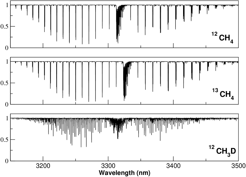
Figure 1: Synthetic absorption at 3.0 microns of the 3 isotopologues of methane available at the HITRAN 2008 database. Methane is a very strong absorber at this wavelength, so cell lengths of a few mm or cm have been used to generate this example spectra (T=300 K, P=300 mb).

In overview, the absorption spectra of ¹⁴NH₃ and ¹²CH₄ can be simulated to a high degree of realism by using the line lists available in the HITRAN 2008 database and a basic ray-tracing software. Concerning the ray-tracing software, we explored several options and found that the Reference Forward Model package (RFM) provided the most straighforward and simplest approach to obtain the desired synthetic spectra. As a cross-check, We compared our simulated spectra with those computed with SpectralCalc, obtaining perfect agreement among the two. As discussed before, the absorption spectra of ¹³CH₄ is obtained to the required level of realism by applying a multiplicative factor to the wavelengths of the ¹²CH₄ spectrum. As will be shown in Sec. 4.2, this approach worked very well in the estimation of the optimal pressure for the ¹³CH₄ cell. Because the absorption spectrum of ¹²CH₃D is very different from ¹²CH₄, we could not perform the same optimization analysis. Since the ¹²CH₃D lines at 3.5 microns are shallower than those from ¹²CH₄, we tentatively filled this cells with a pressure slighty higer than the optimal one found for the ¹³CH₄ cell. As shown later, such pressure turned to be insufficient to produce deep-enough lines. Now that the spectrum of ¹²CH₃D is known, we will be able to use it to optimize future cells. Hereafter, all the optimization details refer only to ¹⁴NH₃ and ¹³CH₄.

2.4 Model Configuration Setup

For the purposes of our optimization models, the length of all the cells is fixed at 10 cm. We also assume an ideal spectrograph continuously covering an interval of 200 nm at the K band. While an instrument with such capabilities does not yet exist, a comparable wavelength coverage should be within the reach of the proposed NIR spectrographs (e.g., i-Shell on NASA’s IRTF, and upgraded versions of NIRSPEC/Keck and CRIRES/VLT). Such wavelength range is also representative of the interval where the cells under discussion (ammonia and methane) show more absorption features in the K band. Note that the cells only provide good wavelength calibration on the spectral region well covered by them so using the full K band to estimate the performance of each cell would seriously underestimate the stellar contribution to the error budget. The central wavelength of the interval is also obtained during the optimization process. Four spectral resolutions are also tested: 30 000, 50 000, 70 000 and 10⁵. These resolutions roughly match the range of available (or planned) nIR spectrographs. To make a fair comparison, we will assume that the number of collected photons is the same in all the setups. In other words, when the resolution is higher, the signal will be spread on a larger number of resolution elements and, therefore, the S/N per resolution element will be reduced. The resulting $\sigma_{V}$ for various setups and gas cell configurations are given in Figure 2. In addition to the cell parameters, the central wavelength $\lambda_{c}$ of the 200 nm window is also optimized. The atmospheric K-band window is surrounded by strong and very variable water absorption features that we want to avoid as much as possible. Neither gas shows enough absorption features below 2100 nm to be useful for wavelength calibration. As a result the useful wavelength range we test is between 2100 and 2450 nm. For the stellar spectra, we have used those provided by the PHOENIX group (Hauschildt et al., 1999). Solar metallicity and a $logg=5.0$ have been assumed in all cases.

3 Model Results

For ¹⁴NH₃, $\sigma_{V}$ is computed on pressures ranging from 25 to 250 mbar in steps of 25 mbars. For ¹³CH₄, the tested pressures go from 50 to 500 mbars in steps of 50 mbars. Figure 2 and Table 1 summarize our results as follows :

• The optimal gas pressure depends on the spectral resolution. When the pressure is too low, the gas column density is also low and the lines are shallower. When the pressure is high, the lines are deeper due to the increased column density, but they get broader due to presure broadening effects. The optimal gas presures for the proposed setups are given in Table 1.

  Table 1: Optimal setup for the various test setups. We use a stellar atmosphere model for a T=3000 K star, and a cell Length of 10 cm.

  	Spectral	S/N/$\delta\lambda$	Nδλ	$\lambda_{c}$	$\sigma_{\rm cell}$	$\sigma_{*}$	$\sigma_{V}$	Pressure
  Gas	Resolution			[nm]	[m s-1]	[m s-1]	[m s-1]	[mb]
  13CH4
  	30 000	182	2370	2370	8.9	12.3	15.1	400
  	50 000	141	4300	2360	6.5	8.0	10.4	300
  	70 000	119	6021	2360	4.8	6.6	8.2	200
  	100 000	100	8602	2362	3.8	5.7	6.9	150
  14NH3
  	30 000	182	2370	2298	16.7	14.0	21.8	150
  	50 000	141	4300	2292	12.4	9.3	15.5	100
  	70 000	119	6021	2298	10.6	7.4	12.9	75
  	100 000	100	8602	2298	8.7	6.5	10.9	50

  

  

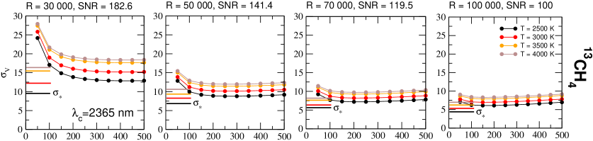
  Figure 2: Photon noise radial velocity precision $\sigma_{V}$ as a function of gas cell pressure for different stellar atmosphere models (colored dots). Because the spectra of stars depends on the effective temperature, $\sigma_{V}$ will also depend on that. Top panels contain the results for the ¹³CH₄ cell and the results for ¹⁴NH₃ are given in the bottom panels. The contribution of the stellar spectra (small horizontal lines on the bottom left of each plot) are also illustrated. Note that the stellar contribution is different for each cell. Because the cells have a higher density of lines on slightly different wavelength ranges, the optimal central wavelength is different for each cell. Such optimal wavelength also weakly depends on the resolution and the gas pressure. The average values of the optimal wavelengths are also given for each setup. In all the cases, ¹³CH₄ nominally outperforms ¹⁴NH₃.

• Even accounting for the reduction in the S/N per resolution element, the higher spectral resolution $R$ always provides higher RV precision. The spectrum of the star and the cell are sufficiently resolved at R=100 000, so higher resolutions do not provide a significant improvement (Mahadevan & Ge, 2009). Note that we are not discussing the slit size required to achieve each resolution. If a fraction of light $L$ is lost due to bad seeing ($>$1.0”) and/or narrow slit (eg. 0.2”), $\sigma_{V}$ has to be divided by $\sqrt{L}$. The photon-collection efficiency (also called throughput) for a given mode heavily depends on engineering details of each spectrograph (slit size, use of an image slicer, adaptive optics, etc.). The loss of throughput can easily counter the gain in precision from the higher spectral resolution. Therefore, one should first compare the relative performance of the available modes before building a cell optimized for the highest spectral resolution available. As a general approach, we suggest first determining the desired $R$ using synthetic stellar spectra and all the information available on the available observing modes. Only then one should proceed to the gas cell optimization for a given R.

• Both the stellar and the cell spectra contribute significantly to $\sigma_{V}$. In the case of ¹⁴NH₃, the absorption cell dominates $\sigma_{V}$. As a consequence, the RV measurements will be calibration-noise-limited. On the other hand, the contribution of ¹³CH₄ to the overall precision is always smaller than the stellar contribution, which makes it more attractive than ¹⁴NH₃.

• ¹⁴NH₃ and ¹³CH₄ cover a different range of wavelengths. Therefore, the optimal central wavelength $\lambda_{c}$ strongly depends on the gas used. To a much lower degree, $\lambda_{c}$ also depends on the spectral resolution and pressure; therefore, the optimal wavelength is always within 5 nm to the values given in Figure 2. Also, ¹³CH₄ covers the stellar CO absorption bands better than ¹⁴NH₃, minimizing $\sigma_{*}$ and therefore further improving the maximum achievable precision.

This latter two items justify the effort of developing a methane-based absorption cell for future high-precision RV measurements in the NIR. As we mentioned before, each resolution element should contain (at least) 2 or more pixels to properly sample the intrumental profile. If the same S/N can be achieved per pixel instead, then the maximal RV precisions $\sigma_{V}$ listed in Table 1 have to be divided by the square-root of the number of pixels per resolution element. That is, with the best setup we tested (R = 100 000, ¹³CH₄, $\sigma_{V}$ = 6.9 m s^-1), a star with T = 3000 K and 2 pixels per resolution element with a S/N = 100 per pixel, one should be able to achieve RV precisions better than 5 m s^-1.

4 Optimal absorption cells for IRTF/CSHELL

We started a pilot program to test the absorption cells at the CSHELL spectrograph installed at the NASA/IRTF telescope (Mauna Kea,Hawaii; Tokunaga et al., 1990; Greene et al., 1993). The design parameters and the optimal setup found for this spectrograph are given in Table 2. In addition to testing their performance, we were also interested in the practical issues involved in the construction, installation and operation of such cells. With this in mind, we built two methane-based cells containing ¹³CH₄ and ¹²CH₃D, as well as a ¹⁴NH₃ cell for comparison purposes. The construction details and the final high-resolution FTIR of the cells are given in Section 4.2. For this experiment, the central wavelength was not optimized. To simplify the analysis required to obtain precise RV measurements, we chose $\lambda_{c}$ = 2312.5 nm which is centered in a small window that is relatively free of telluric methane features (see Section 4.2).

Table 2: Design parameters and optimal setup for IRTF/CSHELL. The stellar model used in the optimization process has T = 3500 K, log g = 4.5 and solar metalicity

Parameter	Value
Spectral resolution	46 000
Cell length	12.5 cm
Cell temperature	283 K
Wavelength interval
at K band	$\sim$ 5 nm
Npix	256
Optimal 13CH4 pressure	275 mb
Optimal 14NH3 pressure	70 mb
Selected $\lambda_{c}$	2312.5 nm
$\sigma_{V}$ (S/N=100/$\delta\lambda$)	$\sim$ 50 m/s-1
$\sigma_{V}$ (S/N=100/pix)	$\sim$ 35 m/s-1

4.1 Construction of the Cells

Here, we summarize the practical details involved in the construction of the three cells filled with ¹³CH₄, ¹²CH₃D, and ¹⁴NH₃. In all cases, the construction of the cells is very affordable.

Based on the limitations imposed by the existing extra space in CSHELL, the bodies of the cells were made using a Pyrex tube 12.5 cm in length and 5.1 cm in diameter. Both ends of this tube were capped with low-OH quartz windows with excellent transmission in the NIR. The windows were then coated on the outside with an infrared antireflective coating to further improve transmission. We did not coat the inside of the windows due to potential chemical reactions of the gas with the coating degrading throughput. Using the laboratory FTIR spectra of all the cells, we found that the overall transmission on the continuum (including the gases) is typically above 80%. Each window is a wedge with an angle of 1.6^∘ oriented 180^∘ relative to the other window on the cell, corresponding to a 2 mm rise in window thickness over 7 cm, with a minimum window thickness at one end of 1 mm. This prevents ghost images from appearing on the stellar spectra which arise from multiple reflections off the spectrograph’s optics. The windows were sealed using Varian Torr Seal, a sealant specifically designed to connect glass and maintain a vacuum for a duration longer than a decade in nominal conditions.

Pure anhydrous ¹⁴NH₃ ammonia was purchased from Matheson-TriGas ($>$99.9% quoted purity). The ¹³CH₄ isotopologue was purchased from Sigma-Aldrich (99% quoted purity). The more exotic ¹²CH₃D isotopologue was obtained from Cambridge Isotope Laboratories, Inc. (98% quoted purity). All three cells were evacuated using a standard vacuum pump, and then filled with the gases. As shown in Table 2, ¹⁴NH₃ and ¹³CH₄ cells were found to operate optimally at $\sim$75 mbar and 275 mbar respectively (as a reference, 1013.25 mbar is 1 atm or 1.013⁵ Pa). Since we had no means to predict the optimal pressure for ¹²CH₃D at the K band, we filled the ¹²CH₃D cell at a higher pressure ($\sim$ 345 mbar), waiting for the FTIR spectra to evaluate if the cell would be suitable for use at CSHELL. The cells were filled at such pressures at 20^o C by means of a small inlet in the side of the pyrex tube. In order to seal this inlet, the gases were then condensed to a liquid via immersion in an ice bath. This allowed the Pyrex inlet to be heated to $\sim$ 1100 K without raising the interior gas temperature and pressure. If the gases had been left in the gas phase at 20^o C, the internal pressure would have exceeded 1 atmosphere and the gas would have burst out of the hot malleable inlet. The first tests filling our gas cells with ammonia gas resulted in this outcome. The end result of the sealing process allowed for the creation of an essentially permanent Pyrex seal to the inlet such that the main body tube is a single piece of Pyrex.

All three cells are interchangeable and can easily be substituted as needed by removing the current cell and placing one of the others in the mount. The active cell is mounted inside a calibration box with an aluminum housing, which in turn sits in front of the CSHELL spectrograph entrance window. The gas cell tube is attached to a rotary stage by aluminum braces which allows the cell to be moved in and out of the telescope’s beam by remote operation (see Fig. 3). The remote operation is an essential design feature for ease of use and efficiency of observations, given that CSHELL mounts at the telescope Cassegrain focus. The cell sits in the converging f/38 beam prior to the beam’s entrance into the spectrograph’s entrance window. Thanks to this, the cell absorption spectrum is imprinted on the stellar light before the light goes into the spectrograph optics. The available physical space limitations for the cell ($\sim$ 15 $\times$15 $\times$18 cm³) placed severe design constraints on the size of the cell and the motor mechanism to move the cell in and out of the telescope beam. The length of the cell is limited on one end by the entrance window to the calibration unit, and on the other end by the descending fold mirror for the calibration lamps.

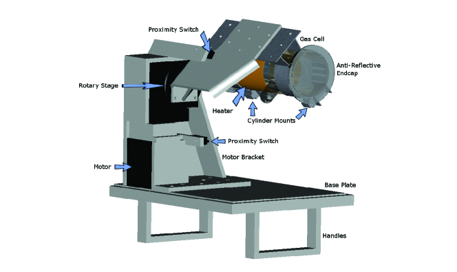
Figure 3: A rendering of the CAD design of the gas cell, rotary stage, and mounting mechanism. Note the heating element and the thickness of the aluminum braces (shown in gray) to maintain rigidity and prevent rotation of the cell for consistent placement in the beam. Wires and bolts are omitted for visual clarity.

The IRTF telescope dome experiences ambient temperature ranges of 276 to 284 K. In order to mitigate velocity calibration errors due to temperature changes of the cell’s gas, its temperature is stabilized with a small silicon heater. For consistency, it is heated to 283 K (10^o C), at the high end of dome temperatures experienced over the past year. The cell has an RTD sensor attached giving temperature feedback to a temperature controller, which is expected to maintain the temperature to within $\pm$0.1 K. The temperature controller can be set and logged remotely to ensure stability. This should result in temperature-induced errors well below 1 m s^-1 (Bean et al., 2010b). As a curiosity, we found that bright telluric standard stars (e.g. Sirius) heat the cell by up to $\sim$0.5^o C before the temperature controller re-establishes an equilibrium gas cell temperature (Figure 4).

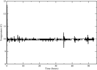
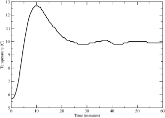
Figure 4: Left: Gas cell temperature stability as a function of hours during first light. Spikes in the temperature can be seen of up to 0.5 C, and are due to observations of very bright standards heating the gas cell. Right: Gas cell temperature as a function of minutes during first hour of turning heater on. The gas cell stabilizes at the desired temperature within 1 hour.

4.2 FTIR spectra of ¹⁴NH₃, ¹³CH₄ and CH₃D

We have obtained laboratory measurements of the three cells’ spectra at the Jet Propulsion Laboratory using a Bruker IFS 125/HR spectrometer, for which the instrumental setup can be found elsewhere (e.g., Sung. et al., 2008; Sung & et al., 2012). The FTIR spectra were taken at a resolution $R\approx 700000$ at 2.0 $\mu$m and 298 K. This resolution is much higher than CSHELL’s resolution of $\sim$46 000, and allows for very precise resolution of the individual spectral absorption features of all three gases. In order to ensure that we had complete coverage of the infrared bands we intended to use, a full scan from 1 to 5 $\mu$m wavelengths was performed. The FTIR system at JPL is equipped with a temperature-stabilized He-Neon laser has enabled a frequency precision better than 0.0001 cm^-1 in the scanned region, where the units of frequency are wavenumbers per unit of length. The internal frequency accuracy is better than 0.01 cm^-1, that would correspond to a Doppler offset of 740 m s^-1 at the K band. Because precision radial velocity measurements are always relative, extreme absolute accuracy (as opposed to precision) is not required for this experiment. If the spectra we provide need to be used for accurate frequency work, the ¹⁴NH₃ and ¹³CH₄ wavelengths can be refined to match the FTIR spectra to the predicted line positions from HITRAN around 3.0 microns where all the species have abundant (and well-documented) spectral features.

We scanned the cell while the FTS was pumped down to 95 to prevent leaks of ammonia which is known to be sticky and notorious in leaving permanent residues on the optical surfaces. This pressure is slightly higher than the cell pressure, minimizing the risk of leaks. For the methane isotopologues, the FTS was evacuated to better than 1 mbar in pressure. For all three cases, we obtained the spectra without the cell at a pressure similar to that of each cell. In this way, the unwanted atmospheric residual features could be canceled out by dividing the cell spectra by their no cell counterparts. The normalized K-band FTIR spectra of the cells are shown in Figure 5. A synthetic spectrum of a T=3000 K star ($\sim$ M5V) is shown on the top for comparison. The second spectrum in Figure 5 is a sample of the Earth’s atmosphere absorption along the K band. Compared to the spectra of ¹³CH₄ (foruth row), it is easy to identify the features due to telluric methane (eg. look for the gap at 2313 nm, that appears at 2321 nm in the ¹³CH₄ spectrum). Water vapor is a major contributor to the telluric absorption beyond 2400 nm. The ¹⁴NH₃ cell is in remarkable agreement with the one obtained by our synthetic spectra generator. As expected, the ¹³CH₄ spectrum looks very similar to the one from ¹²CH₄, which validates our optimization procedure. The ¹²CH₃D spectrum contains a very high density of shallower lines. Even though ¹²CH₃D has a higher density of lines, it is not usable for CSHELL because at $R$ = 46 000, those lines are not deep enough to be competitive against ¹⁴NH₃ or ¹³CH₄. Still, our laboratory-obtained spectra of ¹²CH₃D can now be used to design optimal cells on other spectrographs. Even though the atmospheric contamination is less significant around 2150 nm, neither the gas cell nor the stellar spectra contain many strong absorption features around that wavelength.

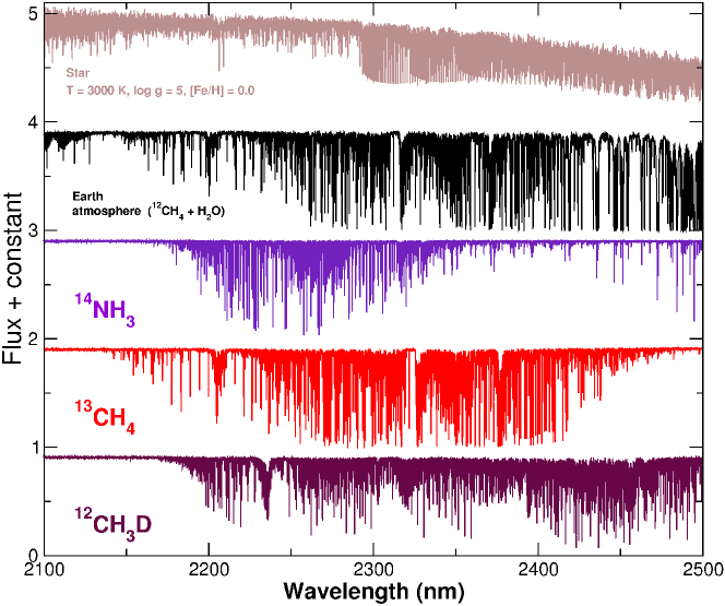
Figure 5: Relevant spectral features in the K band. From top to bottom : synthetic spectrum of an M5V star, absorption spectrum of the Earth’s atmosphere, and laboratory obtained spectra of our cells : ¹⁴NH₃, ¹³CH₄ and ¹²CH₃D (R$\sim$ 700 000).

Our FTIR spectra were obtained at a temperature of 298 K, whereas we are operating the gas cell on the IRTF telescope at a temperature of 283 K. Simulated spectra indicate that the difference in temperature introduces a small systematic offset of the order of 1 m/s or less. While this should not affect our relative RV measurements, the FTIR spectrum of prospective cells should be obtained at the same telescope operation temperature to guarantee that the forward modeling of the observed spectra is as accurate as possible.

4.3 H Band

We show the absorption spectra of our three cells in the H band (see Fig. 6). Similar to K, the H band is surrounded by very variable water vapor features from the Earth’s atmosphere that should be avoided. The central part of the H band is dominated by two prominent bands of CO₂ that are known to be quite stable and have been used to reach precision radial velocities at the level of 10 m s^-1 (Figueira et al., 2010). Both methane isotopologues show abundant lines on the redder part of the band, while ammonia has a very promising band on the bluer part. Even though the ammonia absorption is quite prominent, such band is not listed in HITRAN 2008 so it was a surprise to find it there. Since the gases were not optimized for H band work, the absorption lines of all three cells are too shallow to produce competitive results compared with the K band. Testing the H band would require the construction of additional cells and was beyond the scope of our limited budget for this initial study. There are other gases and isotopologues that provide useful absorption features around 1500 nm. Some of the most promising ones have already been discussed by Mahadevan & Ge (2009) and Valdivielso et al. (2010). From our obtained spectra, a higher-presure cell combining ¹⁴NH₃ and ¹³CH₄ would seem to be a good choice to cover a good fraction of the H band. Because the stellar spectra of cool dwarfs have fewer features than other IR bands (Reiners et al., 2010), and because there are other studies focused on this wavelength range, we do not discuss the H band further.

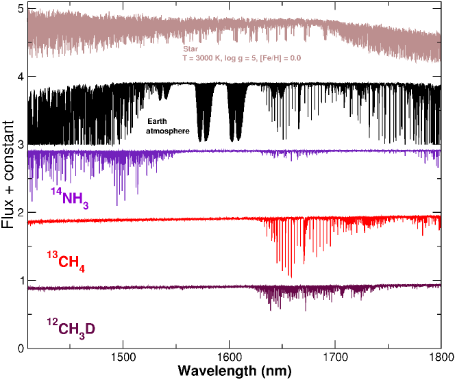
Figure 6: Relevant spectral features on the H band. From top to bottom : synthetic spectrum of an M5V star, absorption spectrum of the Earth’s atmosphere, and laboratory obtained spectra of our cells : ¹⁴NH₃, ¹³CH₄ and ¹²CH₃D (R$\sim$ 700 000).

4.4 First Light

The ¹³CH₄ cell was successfully integrated in the CSHELL spectrograph, and first light was achieved on 15 September 2010. We choose a window centered at $\lambda=2312.5$ nm, because it is almost free of telluric features. The laboratory spectrum of the cell compared with the obtained spectrum of a telluric standard (Vega) through the cell at the telescope is shown in Figure 7. The spectra confirm the presence of the methane in the cell, and a wavelength window relatively free of telluric features. The observed spectra are in excellent agreement with our expectations. We measure an effective FWHM $\delta\lambda\sim$ 1.8 pixels in the wavelength direction. The only prominent telluric line is present at pixel #120. Spectra are extracted from the raw FITS image using a custom pipeline to perform a sum of counts over the spatial direction as a function of wavelength. The exposures were taken at two nodding positions separated by 10 ^′′, which were then subtracted to remove the sky contribution. The raw frames were also cleaned for hot pixels, dead pixels, and cosmic-ray events. Several hundred high S/N spectra (S/N $\sim$ 150, one spectra every 30 seconds) of the supergiant star SV Peg (M7, K mag = -0.4) were also obtained in the first two nights, confirming that both the absorption cell features and the stellar spectrum had abundant lines in the selected wavelength range (see Figure 8).

A preliminary version of our RV extraction pipeline indicates that a precision of $\sim$ 35 m s^-1 can be obtained for each spectrum of SV Peg (see Fig. 9). Our RV determination is based on the forward-modeling technique described by Butler et al. (1996). In brief, we have developed a custom MATLAB code for our analysis. We convolve a model LSF with a model for the intrinsic spectrum of a target star, a model for the telluric spectrum of Earth’s atmosphere (Wallace et al., 1996), the FTIR spectrum for the gas cell, and a foruth-order polynomial model for the continuum. The model LSF consists of a central Gaussian and $N$ satellite Gaussians with adjustable widths, relative amplitudes and centroids to attempt to reproduced the observed variability in the instrumental LSF. We also allow for a variable spectrograph resolution and plate scale along the length of the slit. The residuals between the model and observations are iteratively minimized over the multiple free parameters via a hybrid amoeba simplex algorithm from an initial starting set of parameters that are constrained via a coarse $\chi^{2}$ minimization. We derive a deconvolved template spectrum for the target star using an iterative procedure adding averaged residuals from our fits using the above procedure to observations taken without the gas cell. From the fit parameters, we derive the line of sight radial velocity to a target star from the relative wavelength shift between the model for the gas cell and the stellar template. Using standard barycentric correction routines (Stumpff, 1980), we correct for barycentric motion of the observer to arrive at the final radial velocities obtained on the first two nights of observations as shown in Figure 9. SV Peg was chosen to be very bright and with spectral features in the K band, but it is a M supergiant star and, as such, RV variability at $>10$ m s^-1 level is expected in timescales of a few days. Also, as happens in the optical, obtaining accurate templates is a major limitation of the absorption-cell method. To derive more reliable templates, we are now obtaining very high resolution spectra in the K band using CRIRES/VLT (R$\sim$110 000). The long-term stability of our setup will be demonstrated in a forthcoming publication using observations on known RV stable M dwarfs (e.g., GJ 15A and GJ 293).

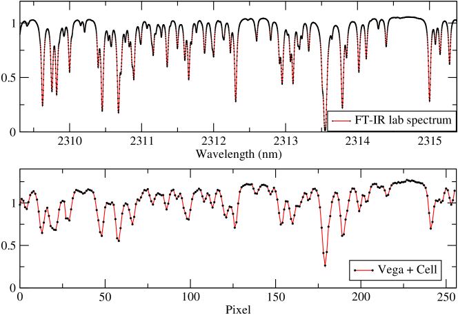
Figure 7: Laboratory FTIR spectrum (top) and observed spectrum (bottom) at IRTF of the ¹³CH₄ cell on the K band window used for CSHELL observations. CSHELL is not cross dispersed and only covers $\sim$ 6 nm at the K band. The only remarkable telluric feature in this window is at pixel 120 and corresponds to telluric methane absorption. The resolution of the FTIR spectrum is 700 000. The lines in the observed spectrum look shallower due to the lower resolution of the spectrograph (R=44 000).

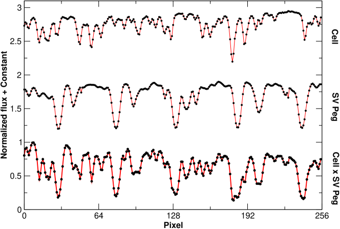
Figure 8: Top. Obtained spectrum of a telluric standard (Vega) observed through the ¹³CH₄ absorption cell. Middle, observed spectrum of the M7 giant star SV Peg observed without the cell. Bottom, Observed spectrum of SV Peg through the cell.

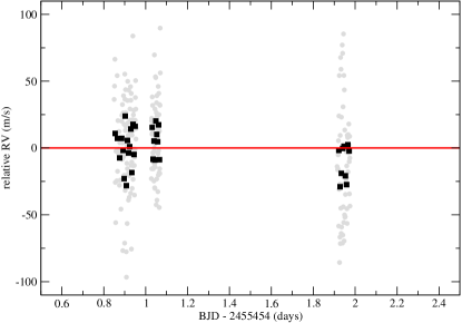
Figure 9: Relative radial velocity measurements of the super giant star SV Peg (K = -0.4) obtained during the first two nights. Each spectra has a formal S/N of about 150. Grey points correspond to individual observations (RMS $\sim 35$ m s^-1). Black points correspond to averaged blocks of 6 observations. The measured RMS of the averaged blocks ($\sim 14.8$ m s^-1) is almost identical from what would be expected from Gaussian white noise ($35/\sqrt{6}=14.2$ m s^-1). SV Peg is a supergiant star and, as such, should show some RV variability in time-scales of a few days and may explain the few m s^-1 offset between the mean of the two nights.

5 Conclusions and Current work

We demonstrated a methodology to design optimal gas cells for precision RV measurements using high-resolution spectrographs. Our numerical experiments showed that, given a high resolution spectrograph covering the K band, precisions better than 5 m s^-1 level can be achieved for late M dwarfs (T$<$3500 K), enabling the detection of terrestrial planets orbiting in their habitable zones. Additionally, precision RVs of earlier type G0 to mid-K dwarfs could also be obtained, enabling planet-search programs around young active stars. We constructed two such methane isotopologue cells and presented FTIR spectra useful for future RV applications and isotopic abundance determination on solar-system studies. We commissioned the ¹³CH₄ gas cell on CSHELL/IRTF, and provided optimal parameters for future spectrographs with the ability to operate in the K band. Even if the final ¹²CH₃D cell was suboptimal for work in the K band, we found that this isotopologue of Methane has an even higher density of lines. Thanks to the obtained FTIR spectra, a cell with ¹²CH₃D can also be now optimized. A similar increase in line density would be expected from a deuterated isotopologue of ammonia (e.g., ¹⁴NH₂D). Unfortunately, no comprehensive line lists exist for such species. We plan to better characterize some of these isotopologues in the future using laboratory FTIR spectroscopy and custom-made cells.

The absorption-cell technique discussed here consists of inserting the cells directly on the optical path of the starlight. Given a stabilized spectrograph (e.g., HARPS/ESO), such cells could also be used as external calibration sources by illuminating them with white light and producing a ‘lamp-like’ calibration spectrum in absorption (see Mahadevan & Ge, 2009, for a more detailed discussion). However, stabilized spectrographs are more expensive to build, tend to be less versatile and none is currently available to work in the NIR. Alternative methods to provide external wavelength calibration have been proposed (e.g., frequency comb and/or a stabilized ethalon), but they will also work on stabilized spectrographs. The absorption-cell technique remains as the only option if precision RV measurements are needed from general-purpose instruments such as NIRSPEC/Keck, CRIRES/VLT or the planned i-Shell/IRTF.

In October 2010, we started a pilot program to obtain RV measurements on late-type young dwarfs (K and M). The targeted radial velocity precision is between 30 to 50 m s^-1 (depending on the spectral type). An end-to-end data analysis pipeline is being developed that applies the forward modeling technique outlined in Butler et al. (1996). Stellar spectra templates at higher resolution (using CRIRES/VLT, R=110 000) are being obtained to be used in the modeling of the observed spectrum. The first results of our survey and the long-term stability of the methane cells will be presented in a forthcoming publication. Preliminary intranight measurements on the giant star SV Peg (K mag $=$ -0.4) indicate that a precision down to 35 m s^-1 (S/N = 150) is within our reach. Let us note that we are only using 6 nm out of 300 nm avaliable in the K band. Preliminary analysis of the most recent observing run (August 2011) confirms that the ¹³CH₄ gas cell pressure and operation remains nominal after nearly one year of operation on the telescope at the summit of Mauna Kea, Hawaii. Given the better nominal performance of methane isotopologues compared to ¹⁴NH₃, and assuming that the photon noise is a significant term in the final error budget, a ¹³CH₄ (or ¹²CH₃D) cell installed on a CRIRES-like spectrograph and a similar setup as the one used by Bean et al. (2010a) should lead to a 30-40% improvement in the overal Doppler accuracy (3-4 m s^-1 precision compared to the current 6 m s^-1 long term accuracy demonstrated on Barnard star and Proxima Cen). (Bean et al., 2010a) discussed that the likely limiting factor of the Ammonia-CRIRES program was contamination by shallow telluric features, both on the observations and during the stellar template reconstruction. While this is a likely source of systematic uncertainty, our numerical simulations indicate that the ammonia cell’s contribution to the error budget has almost the same magnitude as the reported RMS on RV stable stars. We therefore conclude that, even though telluric contamination is a source of uncertainty for sure, using a methane cell on CRIRES should lead to a significant increase in precision. Given that enough space is left between the telescope and the spectrograph ($\sim 10$ cm), such cells can be installed at little cost in upgraded versions of the available NIR instruments (eg. NIRSPEC at Keck, CRIRES/VLT) and planned instruments with K-band capabilities (e.g., i-Shell at NASA/IRTF).

Acknowledgements

Both G. Anglada-Escudé and P. Plavchan contributed equally to this work. G.A. would like to acknowledge the Carnegie Postdoctoral Fellowship Program and the support provided by the NASA Astrobiology Institute grant NNA09DA81A. Peter Plavchan would like acknowledge Wes Traub and Stephen Unwin for funding provided by the JPL Center for Exoplanet Science and NASA Exoplanet Science Institute. K. Sung acknowledges the Planetary Atmospheric Research Program to support the laboratory spectroscopic calibrations. Part of the research at the Jet Propulsion Laboratory (JPL) and California Institute of Technology was performed under contracts with National Aeronautics and Space Administration. We thank Anu Dudhia for making the RFM code available to us and his assistance adapting it for gas cell spectral calculations. The stellar synthetic spectra were graciously provided by Peter Hauschildt (U. of Hamburg) and the PHOENIX group. We also thank Linda Brown from JPL’s Laboratory Studies & Modeling group, and Pin Chen from JPL’s Planetary Chemistry & Astrobiology group for their advice and support using the FTIR spectrometer. We would like to thank Paul Butler (Carnegie Institution of Washington) and Gilian Nave (NIST) for their advice in gas optimization parameters and mollecular spectroscopy in general. We would like to thank Stephen Kane (NExScI), Kaspar von Braun (NExScI), and Steve Osterman (U. of Colorado) for their valuable discussions. We also thank John Rayner, Morgan Bonnet, George Koenig and Alan Tokunaga from IfA/Hawaii for their support during the CSHELL/IRTF cell design review, integration and commissioning. We thank Rick Gerhart (Caltech), Scot Howell (Mindrum Precision) and Thurston Levy (Glass Instruments, Inc.) for their work in helping construct and fill the gas cells, and Joeff Zolkower (Caltech) for mechanical engineering advise.

References

- Bailey et al. (2011) Bailey, J., White, R., Blake, C., et al. 2012, accepted in ApJ, –,
- Bean et al. (2010a) Bean, J. L., Seifahrt, A., Hartman, H. et al. 2010a, ApJ, 711, L19
- Bean et al. (2010b) Bean, J. L., Seifahrt, A., Hartman, H. et al. 2010b, ApJ, 713, 410
- Boudon et al. (2009) Boudon, V., Champion, J., Gabard, T. et al. 2009, Europhys. News., 40, 17
- Butler et al. (1996) Butler, R. P., Marcy, G. W., Williams, E. et al. 1996, PASP, 108, 500
- Charbonneau et al. (2009) Charbonneau, D., Berta, Z. K., Irwin, J., et al. 2009, Nature, 462, 891
- Crane et al. (2010) Crane, J. D., Shectman, S. A., Butler, R. P., et al. 2010, SPIE Conf. Series, Vol. 7735
- Endl et al. (2006) Endl, M., Cochran, W. D., Kürster, M., Paulson, D. B. et al. 2006, ApJ, 649, 436
- Figueira et al. (2010) Figueira, P., Pepe, F., Melo, C. H. F., et al. 2010, A&A, 511, A55+
- Ge et al. (2002) Ge, J., Erskine, D. J., & Rushford, M. 2002, PASP, 114, 1016
- Gillon et al. (2007) Gillon, M., Pont, F., Demory, B.-O., et al. 2007, A&A, 472, L13
- Greene et al. (1993) Greene, T. P., Tokunaga, A. T., Toomey, D. W., & Carr, J. B. 1993, in SPIE Conf. Series, Vol. 1946, p313–324
- Hauschildt et al. (1999) Hauschildt, P. H., Allard, F., & Baron, E. 1999, ApJ, 512, 377
- Howard et al. (2010) Howard, A. W., Marcy, G. W., Johnson, J. A. et al. 2010, Science, 330, 653
- Huang et al. (2008) Huang, X., Schwenke, D., & Lee, T. 2008, J. Chem. Phys., 129, 214304
- Johnson et al. (2007) Johnson, J. A., Butler, R. P., Marcy, G. W., et al. 2007, ApJ, 670, 833
- Kaeufl et al. (2004) Kaeufl, H.-U., Ballester, P., Biereichel, P., et al. 2004, SPIE Conf. Series, Vol. 5492, 1218–1227
- Mahadevan & Ge (2009) Mahadevan, S. & Ge, J. 2009, ApJ, 692, 1590
- Mayor et al. (2009) Mayor, M., Bonfils, X., Forveille, T., et al. 2009, A&A, 507, 487
- McLean et al. (1998) McLean, I. S., Becklin, E. E., Bendiksen, et al. 1998, SPIE Conf. Series, Vol. 3354, p566–578
- Nai-Cheng et al. (1981) Nai-Cheng, S., Yao-Xiang, W., Yi-Min, S., Cheng-Yang, L., Xue-Bin, Z., & Chu, W. 1981, in Precision Measurement and Fundamental Constants, ed. B. N. Taylor & W. D. Phillips, 77–+
- Reiners et al. (2010) Reiners, A., Bean, J. L., Huber, K. F., Dreizler, S., Seifahrt, A., & Czesla, S. 2010, ApJ, 710, 432
- Rivera et al. (2010) Rivera, E. J., Laughlin, G., Butler, R. P., Vogt, S. S., Haghighipour, N., & Meschiari, S. 2010, ApJ, 719, 890
- Rothman et al. (2009) Rothman, L., Gordon, I., Barbe, A., et al. 2009, JQSRT, v110, p533
- Stumpff (1980) Stumpff, P. 1980, A&AS, 41, 1
- Sung. et al. (2008) Sung., K., Brown, L. R., Toth, R. A., & Crawford, T. J. 2008, Canad. J. Phys., 87, 469
- Sung & et al. (2012) Sung, K., Brown, L.R., Huang, X. et al. 2012, JQSRT, in print
- Tokunaga et al. (1990) Tokunaga, A. T., Toomey, D. W., Carr, J., Hall, D. N. B., & Epps, H. W. 1990, SPIE Conf. Series, Vol. 1235, p 131–143
- Urban et al. (1989) Urban, Š., Tu, N., Narahari Rao, K., & Guelachvili, G. 1989, Journal of Molecular Spectroscopy, 133, 312
- Valdivielso et al. (2010) Valdivielso, L., Esparza, P., Martín, E. L., Maukonen, D., & Peale, R. E. 2010, ApJ, 715, 1366
- Vogt et al. (2010) Vogt, S. S., Butler, R. P., Rivera, E. J., Haghighipour, N., Henry, G. W., & Williamson, M. H. 2010, ApJ, 723, 954
- Wallace et al. (1996) Wallace, L., Livingston, W., Hinkle, K., & Bernath, P. 1996, ApJS, 106, 165
- Yurchenko et al. (2005) Yurchenko, S. N., Zheng, J., Lin, H., Jensen, P., & Thiel, W. 2005, J. Chem. Phys., 123, 134308
- Zechmeister et al. (2009) Zechmeister, M., Kürster, M., & Endl, M. 2009, A&A, 505, 859